
10
An Introduction to the Lyapunov Stability of Nonlinear Fractional Order Systems
10.1. Introduction
In automatic control, the main interest of the Lyapunov approach concerns the stability analysis of nonlinear systems. Many works are devoted to this topic, particularly those reported in three famous monographs [SLO 91, KHA 96, SAS 10], which can be considered as references. As it was highlighted previously (see Chapter 8), the Lyapunov stability of nonlinear fractional systems has motivated many conference and journal papers, long before the linear case receives a satisfying solution [MOM 04, FAH 12, WAN 09, CHE 14, LI 14, HUL 15]. A famous paper [LI 09, LI 10], which has been cited in many other papers [SAD 10, FAH 11], is a good example of these publications. It deals with the stability of nonlinear fractional systems, based on the concept of Mittag-Leffler stability. In fact, it is the adaptation to the fractional case of a work by Khalil [KHA 96]. However, as the question of the system initial conditions, obviously fundamental either in the integer order case or the fractional case, relies on Caputo’s definition, this approach is questionable with respect to its generalization.
Therefore, according to our approach in this monograph, we intend to propose an introduction to the Lyapunov stability of nonlinear fractional systems, certainly modest, but motivated by a concern for rigor, based on the main results of the linear case.
As the nonlinear domain is a large topic, the main definitions will not be mentioned here; therefore, the reader is referred to previous monographs [SLO 91, KHA 96, SAS 10]. Moreover, this introduction is restricted to nonlinear autonomous system, characterized by the nonlinear differential equation:
with either commensurate or non-commensurate orders.
This introduction begins with the indirect Lyapunov method, based on a local approximation around the equilibrium point, which makes it possible to test system local stability.
The choice of an appropriate Lyapunov function is a fundamental problem of the nonlinear case, either integer order or fractional order [LYA 07, LAS 61, KRA 63]. This methodology is usually known as the direct Lyapunov method. The variable gradient method [GIB 63] makes it possible to build such a Lyapunov function. We intend to demonstrate how this methodology can be adapted to the fractional case, using two examples [TRI 11b].
Finally, we consider non-commensurate and nonlinear fractional order systems, using the energy balance approach used in the previous chapter. This presentation is based on the well-known Van der Pol oscillator example [KHA 96, MUL 09]. Our methodology makes it possible to define the stability condition and to propose an approximate characterization of the limit cycle [MAA 16].
10.2. Indirect Lyapunov method
10.2.1. Introduction
The indirect Lyapunov method is based on a local approximation of the nonlinear system around its equilibrium point [KHA 96]. It makes it possible to conclude on the local stability of this equilibrium point. We propose an adaptation of this methodology to nonlinear commensurate order fractional systems.
10.2.2. Linearization
Consider the nonlinear commensurate order fractional system
Let ![]() be the equilibrium point.
be the equilibrium point.
Therefore, the nonlinear system is linearized around ![]() using the development of
using the development of
Since the terms linearly depending on ![]() are in
are in ![]() ,
, ![]() decays more than
decays more than ![]() (see Figure 10.1), i.e.
(see Figure 10.1), i.e.
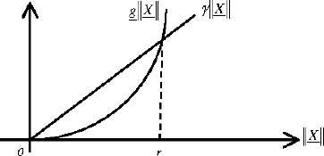
Figure 10.1. Comparison of  and
and 
This means that for any ![]() , we have
, we have
10.2.3. Nonlinear system analysis
System [10.2] is equivalent to
corresponding to the linearized model
In the vicinity of ![]() , system [10.6] behaves as [10.7].
, system [10.6] behaves as [10.7].
System [10.6] can be expressed using a distributed model with internal variables Ẕ(ω, t):

Let V(t) be the Lyapunov function of a commensurate order fractional system (see Chapter 8):
Then
Therefore

Note that ![]() is a scalar.
is a scalar.
Therefore
Then

Note that
Therefore, using the Schwarz inequality [KHA 96, SCH 98]
Thus, we can write

Since (see Figure 10.1)
we obtain
Therefore, we can write

If the eigenvalues of A are negative or with a negative real part, then (ATP + PA) < 0 with P = PT > 0, which means that the linearized system [10.7] is stable ∀n 0 < n < 1.
The term ![]() (or
(or ![]() ) limits the negative value of
) limits the negative value of ![]() in [10.13] (or in [10.19]). Thus, there is a limit value of γ > 0 such that
in [10.13] (or in [10.19]). Thus, there is a limit value of γ > 0 such that ![]() is no longer negative and the nonlinear system [10.2] is unstable.
is no longer negative and the nonlinear system [10.2] is unstable.
Let us recall that for N = 2 (see Chapter 8), we have demonstrated that ![]() can be positive (when the real parts of the eigenvalues of A are positive) but
can be positive (when the real parts of the eigenvalues of A are positive) but ![]() remains negative thanks to the term
remains negative thanks to the term  (caused by dissipation in the fractional integrators – see Chapter 9). This means that there is a limit value of γ such that the nonlinear system remains stable, with a damped oscillating behavior, depending on the value of the fractional order n (0 < n < 1).
10.2.4. Local stability of a one-derivative nonlinear fractional system
Consider the nonlinear system [TRI 11b]:
with
Therefore
and
i.e.
which is presented in the graphs of Figure 10.2.
Note that 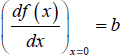 , where x = 0 is the equilibrium point.
Therefore, we can write
The linearized system corresponds to

Figure 10.2. System nonlinearity
The nonlinear system [10.20] corresponds to the distributed model
Consider the Lyapunov function
Thus
and the linearized system corresponds to
This linearized system is stable since b < 0.
The nonlinear system remains stable as long as
or
ie. if
which corresponds to
REMARK 1.– Using the notations of section 10.2.3, we can compare ![]() and
and ![]() , i.e. bx(t) and ax3 (t) (see Figure 10.1).
, i.e. bx(t) and ax3 (t) (see Figure 10.1).
Thus, we can write
with
Then
Thus
which defines the stability domain of [10.20] (see Figure 10.3).

Figure 10.3. Stability domain
10.3. Lyapunov direct method
10.3.1. Introduction
The Lyapunov direct method relies on the appropriate choice of a Lyapunov function V(t), allowing the analysis of global stability: obviously, it is a very large domain of research [LAS 61, KRA 63]. The variable gradient method, proposed by Schultz and Gibson [GIB 63, NAS 68, SLO 91], provides a response to this problem. After a recall of this methodology in the integer order case, we propose to adapt it to the fractional order case, using two numerical examples.
10.3.2. The variable gradient method
A scalar function ![]() is connected to its gradient
is connected to its gradient ![]() through the integral
through the integral
where
The reconstruction of ![]() from its gradient requires that its components verify the curl condition [KOR 68]
from its gradient requires that its components verify the curl condition [KOR 68]

The principle of the variable gradient method is to assume a specific form for the gradient ![]() instead of assuming a form for the Lyapunov function
instead of assuming a form for the Lyapunov function ![]() .
.
A simple solution is to assume that the gradient is of the form
where the coefficients ai,j have to be determined.
This leads to the following procedure:
10.3.3. Nonlinear system with one derivative
Consider again the example of section 10.2.4:
with
In the monovariable case, ![]() has only one component.
has only one component.
The distributed model is

We have to separate the monochromatic Lyapunov function v(ω, t) [TRI 11b] and the global one V(t) such that
Let ![]() be the gradient of v(ω, t) and assume that
be the gradient of v(ω, t) and assume that
Then

Finally, using [10.46], we obtain

Thus
The first term is always negative for α > 0. We have previously demonstrated that a linear system with one fractional derivative (Chapter 8) is stable if the second term is itself negative.
Thus, it is necessary to check whether
or equivalently
i.e.
In addition, we have to determine v(ω, t) and V(t).
Then
Therefore
The function V(t) is positive definite if α > 0 (with α arbitrary).
The nonlinear system [10.43] is globally stable if x(t) verifies the condition
This condition is the same as the condition in example 10.2.4.
REMARK 2.– It is important to note that the stability condition [10.56] is conservative because it does not take into account the influence of z(ω, t) in the negative term  of equation [10.50].
In order to remove this conservatism, it would be necessary to analyze the influence of initial conditions on stability, i.e. z(ω, 0) with this example.
However, it is another fundamental issue, which is beyond the limited objectives of Chapter 10.
10.3.4. Nonlinear system with two fractional derivatives
Consider the commensurate order nonlinear system

This model is derived from the model proposed by Shultz and Gibson [GIB 63].
Its distributed model, with internal variables z1(ω, t) and z2(ω, t), is

Let v(ω, t) be the monochromatic quadratic function, depending on the frequency ω, and V(t) be the global Lyapunov function
Let us define
We know that
Let us define

Assume that ![]() is of the form
is of the form
with
It is possible to impose a22 = 2 (see [GIB 63, SLO 91]).
Then, [10.61] can be written as

Since
we obtain

Let us define
Then

Note that (it will verify a posteriori):
Therefore

Let us return to ![]() .
.
According to [10.63], we obtain

Let us define the Jacobian of ![]()

Ψ has to verify the curl condition [10.41], i.e. ![]() .
.
Since ![]() and
and ![]() , we have to impose
, we have to impose
Let us define a priori a12 = a21 =1, then
We obtain v(ω, t) using equation [10.61]
REMARK 3.– x1(t) is computed from z1(ω, t) using the weighted integral of [10.58], idem for x2(t).
Therefore, x1(t) is a “constant” (with respect to ω) considering z1(ω, t), idem for x2(t) considering z2(ω, t).
We calculate the integral [10.76] defining a path from {0,0} to {z1(ω, t), z2(ω, t)}.
Let
Therefore

Finally

Let us note that
Thus
It is easy to verify that for P > 0, V(t) is a positive definite quadratic form.
We can verify the previous calculation.
With ![]() and a12 = a21 = 1, we obtain
and a12 = a21 = 1, we obtain

i.e.

This means that
Thus, the nonlinear system [10.57] is globally stable.
10.4. The Van der Pol oscillator
10.4.1. Electrical nonlinear system
The electrical nonlinear system is presented in Figure 10.4. It corresponds to a fractional differential system, where Lf is a fractional inductor

It is a negative resistance oscillator [KHA 96, AUV 80, CHA 82], which is characterized by the nonlinear equation i = f(v)
![]() , where –R is a negative resistor.
, where –R is a negative resistor.

Figure 10.4. Fractional Van der Pol oscillator
10.4.2. Van der Pol oscillator
The nonlinear system [10.85] is modeled with two variables iL(t) and v(t). The elimination of iL(t) leads to the classical Van der Pol equation [KHA 96, PET 11] in connection with chaotic systems [HAR 95, STR 15].
since δi = G(v) δv, we obtain
Using
we obtain the standard fractional Van der Pol equation [BAR 07]
10.4.3. Simulation of the nonlinear system
System [10.85] is more general than equation [10.88], and better suited for its analysis and simulation by the energy balance approach (Chapter 9). A first objective is to simulate its dynamical behavior. This system can be written as

Then, using the distributed variable z(ω, t) associated with the fractional integrator ![]() , the first equation of [10.92] is equivalent to
, the first equation of [10.92] is equivalent to

This system is frequency discretized using the technique presented in (see Chapter 2 of Volume 1). Thus, we can simulate the nonlinear system.
10.4.4. Limit cycle
Simulation is performed with the following values [MAA 16]:
Thus, we obtain the different phase portraits of the Van Der Pol oscillator.
In Figure 10.5, the limit cycles are plotted with increasing values of order n, from 0.5 to 1, with α = 1 and the initial conditions v(0) = 0.5 z(ω, 0) =0 ∀ω. In Figure 10.6, for a fixed value of the order (n = 0.5), the same limit cycles are plotted with increasing values of α, from 0.9 to 5.

Figure 10.5. Influence of the fractional order n. For a color version of the figures in this chapter see www.iste.co.uk/trigeassou/analysis2.zip
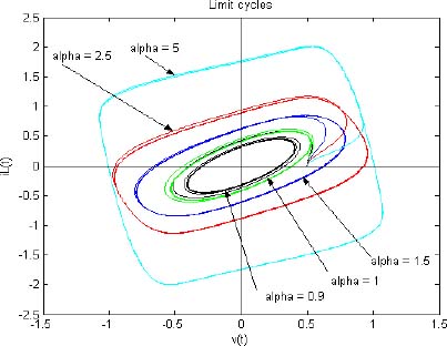
Figure 10.6. Influence of the parameter α
For n close to 1, and large values of α, the limit cycles correspond to the usual Van der Pol ones (see [BAR 07]). On the contrary, for lower values of α, the limit cycles are approximately ellipsoidal and require α > αlim.
Therefore, the objective of the next sections is to analyze and predict these results.
10.5. Analysis of local stability
10.5.1. Linearization
The nonlinear system [10.85] can be expressed as

The equilibrium point of the nonlinear system is ![]() .
.
Let us define

Thus, the linearized system corresponds to

10.5.2. Local stability
Let us define the Lyapunov function (see Chapter 9)
V(t)=EL(t) + EC(t) with
Therefore, the derivative of the Lyapunov function is
Let us recall (Chapter 9) that the first term represents the distributed internal Joule losses of the fractional inductor, whereas the second term corresponds to external Joule loss in the negative resistor G(0) = –α = –1/R.
This Joule loss compensates the internal losses in Lf when
Thus, a constant amplitude oscillation v(t) = Vejγt appears, where γ is the oscillation frequency.
10.5.2.1. Derivation of frequency oscillation
At the stability limit (Chapter 9)
and v(t) = Vejγt.
According to Chapter 9, we obtain
Therefore
thus
Since (Appendix A.9.3.)

and ![]()
we obtain the oscillation frequency

10.5.2.2. Stability condition
The system remains stable if ![]() . This condition is equivalent to
. This condition is equivalent to
αlim is obtained at the stability limit, using equation [10.105].
Since (Appendix A.9.3.):

we obtain

The system remains stable if α < αlim.
REMARK 4.– If n = 1, then αlim = 0. Thus, in the integer order case, the Van der Pol oscillator is unstable ∀ α ≥ 0. On the contrary, the instability of the fractional Van der Pol oscillator requires the condition α ≥ αlim.
10.5.3. Validation of stability results
Consider the numerical values
Then, equations [10.108, 10.111] provide

Figure 10.7. Stability of the Van der Pol system
In Figure 10.7, the limit cycles {iL(t),v(t)} for α = { 0.4; 0.8;1 } are plotted with the initial conditions v(0) = 0.25; z(ω, 0) = 0 ∀ ω.
For α = 0.4 < αlim, we observe that the nonlinear system is stable.
For α = 0.8 ≈ αlim, the system is at the stability limit; therefore, we obtain a constant amplitude sinusoid v(t)=Vejγt characterized by an ellipsoidal phase portrait. Note that the amplitude of this ellipse depends on the initial conditions.
Then, for α = 1 > αlim, the system is unstable, and the amplitude of the limit cycle is independent of the initial conditions.
10.6. Large signal analysis
10.6.1. Introduction
Small signal analysis has demonstrated that the Van der Pol oscillator provides a constant amplitude oscillation v(t) = Vejγt for α = αlim. For α ≥ αlim, this oscillation is nonlinear and characterized by a limit cycle. Consequently, our objective is to determine the amplitude Vlc of this oscillation when v(t) remains approximately sinusoidal, i.e. for the small values of α.
10.6.2. Approximation of the first harmonic [MUL 09]
When v(t) remains approximately sinusoidal, we can still use the expression v(t)=Vejγt. For α = αlim, the amplitude V depends on the initial conditions v(0) and z(ω, 0). On the contrary, for α > αlim, the amplitude depends on the characteristics of i = f(v), independently of the initial conditions.
Let
Since
we obtain
The nonlinear term V3 sin3(γt) can be expressed in terms of harmonics γ and 3γ:
The first harmonic hypothesis leads to
10.6.3. Lyapunov function and oscillation frequency
As described previously, V(t) = EL(t) + EC(t).
Since ![]() , we obtain
, we obtain
with
The oscillation frequency is derived from the equality ![]() . Since the amplitude of v(t) has no influence on the calculus of γ (in the first harmonic hypothesis), the oscillation frequency remains the same as in the linear case, thus
. Since the amplitude of v(t) has no influence on the calculus of γ (in the first harmonic hypothesis), the oscillation frequency remains the same as in the linear case, thus

On the contrary, the amplitude V acts in the expression of Joule losses corresponding to ![]() .
.
10.6.4. Amplitude of the limit cycle
Equality of Joule losses corresponds to
Since [10.120]
In the hypothesis
we obtain
The first harmonic hypothesis leads to
Thus
Therefore, condition [10.122] leads to
Then, the amplitude Vlc of the limit cycle is given by
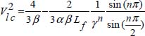
Finally, since v(t) = Lf Dn(iL(t)) and v(t) = Vejγt, we obtain
Consequently, the phase portrait {iL(t),v(t)} is exactly an ellipse in the first harmonic hypothesis.
10.6.5. Prediction of the limit cycle

Figure 10.8. Nonlinear characteristic i=f(v)
In Figure 10.8, the graphs of {i(t),v(t)} for n = 0.5 and v(0) = 0.5; z(ω, 0) = 0 ∀ ω are plotted with increasing values of α. Thus, we obtain the graphs of the function i = f(v) indexed by α. The first harmonic approach remains valid if v(t) does not exceed the limits of the negative resistor zone characterized by ![]() , i.e. by
, i.e. by
Then, using equations [10.129, 10.130] with Lf= 1; C=1; n=0.5; β=1 and α=1, we obtain Vlc=0.525 < 0.577 and ILlc=0.589.
Experimentally (see Figure 10.6), we obtain Vlc=0.527 and ILlc =0.58. Note that the limit cycle is quasi-ellipsoidal; therefore, the first harmonic approach provides a good approximation of the dynamical behavior.
On the contrary, for α = 1.5, the theoretical values are Vlc = 0.792 > 0.577 and ILlc=0.889, and the experimental values are Vlc=0.79 and ILlc=0.85.
Since Vlc > 0.577, the limit cycle is no longer ellipsoidal, and the predicted values are only approximate, as demonstrated in Figure 10.6.
Note that better approximations of the oscillation frequency and the limit cycle characteristics can be obtained by association of the energy balance and harmonic balance approaches [KUN 86].