4
Goal-Oriented Adaptation for Inviscid Steady Flows
The purpose of this chapter is to introduce a mesh adaptation method, which will be closer to the objective of reducing the approximation error, taking into account the discretization of the PDE. In the goal-oriented approach, the user specifies a particular scalar output of the computation. The error in approximating this output through the discretization of the PDE is minimized. The goal-oriented approach relies on (1) a residual/local error estimate in terms of the metric, and (2) an adjoint state relating this estimate to the functional. The use of a continuous metric parameterization permits to build a smooth optimization problem solved via an optimality system. This method is an important method for this book. It is first explained for the case of steady Euler flows with application to sonic boom calculations.
4.1. Introduction
In the previous chapters, the adaptive specification of the mesh is mainly deduced from an interpolation error estimate for some fields (the sensors or the features) related to the PDE solution. Focusing on these interpolation errors is a limitation of this study. If for many applications, the simplicity of this standpoint is an advantage, there are also many applications where feature-based adaptation is far from being optimal regarding the way the degrees of freedom are distributed in the computational domain. Indeed, minimizing the interpolation error is not often so close to the actual objective that consists of obtaining the most accurate approximate solution of a PDE. This is particularly true in the many engineering applications where a specific scalar output needs to be accurately evaluated, for example, lift, drag and moment in aeronautics. Focusing on the best accuracy of such a scalar output is the purpose of goal-oriented mesh adaptation methods, which will take into account both the solution and the PDE in the error estimation, through error estimate and adjoint state. The formulation of goal-oriented mesh adaptation (Becker et al. 1999; Braack and Rannacher 1999; Becker and Rannacher 1996; Giles 1997a; Giles and Pierce 1999; Giles and Suli 2002a; Pierce and Giles 2000; Venditti and Darmofal 2002, 2003) has brought many improvements in the formulation and the resolution of mesh adaptation for PDE approximations. Let us write the continuous PDE and the discrete one as follows:
We focus on deriving the best mesh to approximate a given functional j depending on the solution w. In other words, we examine how to minimize the approximation error δj committed in the evaluation of the functional j:
This objective must be distinguished from deriving the optimal mesh to minimize a global approximation error ‖w − wh‖. See Becker and Rannacher (1996); Verfürth (1996) for a posteriori error estimates devoted to this latter task and Chapter 6 for an a posteriori standpoint. To simplify our goal-oriented formulation, we assume that the functional j is enough regular to be replaced by its Jacobian g. We simplify it as follows1:
We also assume for simplicity that there is no discrete error evaluation on j; this means that jh(wh)= j(wh) 2. On this basis, we seek for the mesh H that gives the smallest error for the evaluation of j from the solution wh:
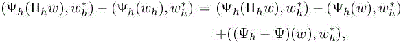
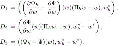
where w and wh verify state equations [4.1]. With statement [4.3], the mesh adaptation problem is recast to an optimization problem. In order to go one step forward in the analysis, we need to implicitly take into account constraint [4.1] in problem [4.3]. The initial approximation error on the cost functional |(g, wh) − (g, w)| can be simplified in terms of a local error Ψ(wh) because of the introduction of the adjoint state w∗:
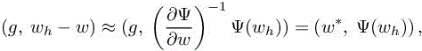
where w∗ is the solution of
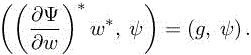
In practice, the exact adjoint w∗ is not available. By introducing an approximate adjoint ![]() weget
weget
4.1.1. What to do with this estimate?
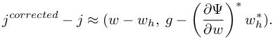
The right-hand side is a spatial integral, the integrand of which should be used to decide where to refine the mesh. The iso-distribution of the error can be approximated by refining according to a tolerance, as in Becker and Rannacher (1996). In Giles and Suli (2002a), it is proposed to use this right-hand side as a correction that importantly improves the quality (in particular the convergence order) of the approximation of j by setting
However, by substituting w∗ by ![]() we introduce an error in
we introduce an error in ![]() which results in being the main error term when we use jcorrected. In Venditti and Darmofal (2002, 2003), it is proposed to keep the corrector and to adapt the mesh to this higher order error term, that is,
which results in being the main error term when we use jcorrected. In Venditti and Darmofal (2002, 2003), it is proposed to keep the corrector and to adapt the mesh to this higher order error term, that is,
or, equivalently,
 [4.5]
[4.5]In order to evaluate numerically these terms, Venditti and Darmofal (2002, 2003) chose to approach these approximation errors, that is, ![]() and wh − w, by interpolation errors:
and wh − w, by interpolation errors:
relying on the differences between the linear representation ![]() and a quadratic representation
and a quadratic representation ![]() reconstructed on a finer mesh.
reconstructed on a finer mesh.
4.1.2. Adjoint-L1 approach
In the approach described in this chapter, metric analysis and goal-oriented analysis are complementary. Indeed, a metric-based method specifies the object of our search through an accurate description of the ideal optimal mesh, while a goal-oriented method specifies precisely the purpose of the search, specifying which error will be reduced. It is then very motivating to seek for a combination of both methods, with the hope of obtaining a metric-based specification of the best mesh for reducing the error committed on a target functional. A few works address this purpose. In Venditti and Darmofal (2003), an anisotropic step relying on the Hessian of the Mach number is introduced into the a posteriori estimate. In Rogé and Martin (2008), an ad hoc formula gives a better impact to the anisotropic component. This chapter presents a different approach to the combination of Hessian and estimates.
The first key point is to work in a continuous (non-discrete) formulation by following the continuous interpolation analysis described in Chapters 3 and 4 of Volume 1. But feature-based metric methods minimize an interpolation error, the deviation between an exact sensor and its linear interpolation on the mesh. This assumes the knowledge of the solution; this is an a priori standpoint. In contrast, goal-oriented methods are generally envisaged from an a posteriori standpoint; we refer to Becker and Rannacher (1996), Verfürth (1996), Apel (1999), Giles and Suli (2002a), Picasso (2003), Formaggia et al. (2004). With that option, the error committed is element-wise known on the mesh under study. Mesh refinement scheme based on a such a posteriori estimations relies on an equi-distribution principle and is thus intrinsically isotropic. Fortunately, goal-oriented methods do not need to be systematically associated with an a posteriori analysis. According to Babuška and Strouboulis (2001), a priori analysis can bring many useful information. Check these information such as anisotropy (see Formaggia and Perotto 2001). This chapter will demonstrate that the goal-oriented error can be globally expressed by an a priori analysis containing anisotropy information. For exploiting this information, a third key point is to work with a numerical scheme that allows expressing the difference Ψh(w) − Ψ(w) in term of interpolation errors. This can be done in a straightforward way by considering finite-element variational formulations.
4.1.3. Outline
This chapter begins with the introduction of a theoretical abstract framework in section 4.2. Within this framework, a first a priori goal-oriented error estimate (equation [4.10]) is derived. Its application to the compressible Euler equations is then studied in section 4.3 for a class of specific Galerkin-equivalent numerical schemes. From this study, a generic anisotropic error estimate (equation [4.13]) is expressed. The estimate is then minimized globally on the abstract space of continuous meshes (section 4.4). We give in section 4.5 some details on the main modifications of the adaptive loop as compared to classical Hessian-based mesh adaptation. The practical optimal metric field minimizing the goal-oriented error estimate is then exhibited. 3D detailed examples conclude this chapter by providing a numerical validation of the theory (section 4.6).
4.2. A more accurate nonlinear error analysis
An accurate error analysis cannot be done without specifying the operator which permits to pass from continuous to discrete and vice versa. Since the P1 interpolate Πh is the pivot of today’s metric analysis, this operator is naturally used in our analysis.
4.2.1. Assumptions and definitions
Let V be a Hilbert space of functions. We write the state equation under a variational statement:
where the operator (, ) is the Hilbertian product, and w is the solution of this equation. Symbol (Ψ(w),φ) holds for a functional that is linear with respect to test function φ but a priori nonlinear with respect to w. The continuous adjoint w∗ is solution of
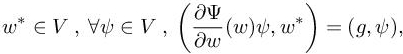
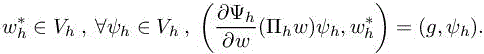
where g is the jacobian of a given functional j. Let Vh be a subspace of ![]() of finite dimension N, and we write the discrete state equation as follows:
of finite dimension N, and we write the discrete state equation as follows:
Then, we can write
For the a priori analysis, we assume that the solutions w and w∗ are sufficiently regular to be interpolated:
and that we have an interpolation operator:
4.2.2. A priori estimation
We start from a functional defined as: j(w) =(g, w), where g is a function of V. Our objective is to estimate the following approximation error on the functional:
as a function of continuous solutions, continuous residuals and discrete residuals. The error δj is split as follows:
δj is now composed of an interpolation error and an implicit error, Πhw − wh. Let us introduce the following discrete adjoint system:
We derive the following extension of δj with the choice ψh = Πhw − wh:
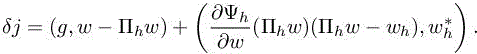
According to [4.9], we have
which gives, by using a Taylor extension,
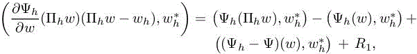
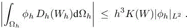
where the remainder R1 is

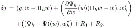
Thus, we get the following expression of δj:
We now apply a second Taylor extension to get

with remainder term

This implies
In contrast to an a posteriori analysis, this analysis starts with a discrete adjoint . ![]() However, our purpose is to derive a continuous description of the main error term. Thus, we get rid of the discrete solutions in the dominating terms. To this end, we re-write δj as follows:
However, our purpose is to derive a continuous description of the main error term. Thus, we get rid of the discrete solutions in the dominating terms. To this end, we re-write δj as follows:
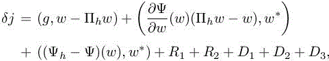
where
The latter expression of δj can be even more simplified because of the continuous adjoint of equation [4.8], leading to
At least formally, the Ri and the Dk are higher order terms, and the first term in the right-hand side of [4.10] is the dominating one. In order to exhibit, from [4.10], a formulation specifying the optimal mesh, we need to make the physical and numerical models more precise.
4.3. The case of the steady Euler equations
In this section, we study how equation [4.10] can be transformed in the context of the steady Euler equations. We restrict to the particular discretization of Chapter 1 of Volume 1.
4.3.1. Variational analysis
Equation [1.5] from Volume 1 will play the role of equation [4.7] in the abstract analysis of the previous section. For the discretisation, we consider a discrete domain Ωh and a discrete boundary Γh, which are not necessarily identical to the continuous ones. The MUSCL scheme introduced in Chapter 1 of Volume 1 can be written as a variational Galerkin-type scheme complemented by a higher order term, which can be assimilated to a numerical viscosity term Dh. This gives, ∀ϕh ∈ Vh,

The numerical diffusion term is of higher order as soon as it is applied to the interpolation of a smooth enough field W on a sufficiently regular mesh (see Mer 1998 for a detailed analysis):
As a result, the dissipation term will be neglected in the same way we neglect the remainders Ri and Dk of relation [4.10]. Even in the case of a flow with shocks, we get inspired by the Hessian-based study of previous chapters and choose to neglect the error term from artificial dissipation.
4.3.2. Approximation error estimation
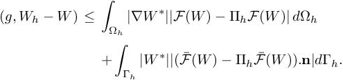
Returning to the output functional j(W) = (g, W) and according to estimate [4.10], the main term of the a priori error estimation of δj becomes
where W∗ is the continuous adjoint state. Using the exact solution W in equations [1.5] and [4.11] while neglecting the dissipation Dh leads to
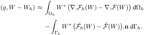
By integrating by parts the previous estimate, we get
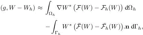
where fluxes ![]() are given by
are given by
By definition, Fh is the linear interpolate of F, that is,ΠhF = Fh, thus we have

We observe that this estimate of δj is expressed in terms of interpolation errors for the fluxes and in terms of the continuous functions W and W∗. The integrands in [4.12] contain positive and negative parts, which could compensate for some particular meshes. In our strategy, we prefer to avoid these parasitic effects in our estimate3. To this end, all integrands are bounded by their absolute values:
4.4. Error model minimization
Starting from the bound in [4.13], several options are possible to derive an optimal mesh for the observed functional. We propose to work in the continuous mesh framework by building a completely continuous estimate, which is possible with the a priori estimate standpoint. It allows us to define proper differentiable optimization (Arsigny et al. 2006; Absil et al. 2008) and use the calculus of variations that is undefined on the class of discrete meshes. This framework lies in the class of metric-based methods. Working in this framework enables us, as in the previous section, to write estimate [4.13] in a continuous form:
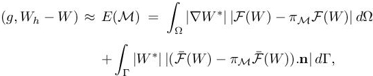 [4.14]
where ![]() is a continuous mesh defined by a Riemannian metric field and
is a continuous mesh defined by a Riemannian metric field and ![]() is the continuous linear interpolate defined hereafter. We are now focusing on the following (continuous) mesh optimization problem:
is the continuous linear interpolate defined hereafter. We are now focusing on the following (continuous) mesh optimization problem:
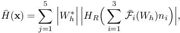
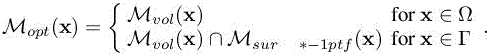
A constraint is added to the previous problem in order to bound mesh fineness. In this continuous framework, we impose the metric complexity to be equal to a specified positive integer N. Let us split the functional E(M) into a volumic functional and a surfacic one. To the minimization of both correspond an optimal metric made of a volume tensor field Mgo defined in Ω and a surface optimal metric ![]() defined on Γ. This is performed as follows:
defined on Γ. This is performed as follows:
– For any x of Ω, the pseudo-Hessian matrix arising from the Euler fluxes is written as
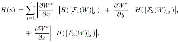
with ![]() denoting the jth component of the vector
denoting the jth component of the vector ![]()
– For any x of Γ, the pseudo-Hessian matrix arising from the surface contribution is written as
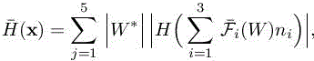
where n = (n1,n2, n3) is the outward normal of Γ.
We can separately apply the optimum computation of section 4.4.1 in Chapter 3 to the two functionals
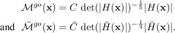 [4.16]
Constants C and ¯C depend on the desired complexity N.
4.5. Adaptative strategy
By freezing the continuous solution, we have in some manner linearized the continuous metric problem, that is, made the error quadratic and got an intermediate optimal metric with a close formula. The optimal metric, solution of the continuous goal-oriented mesh adaptation problem, is the fixed point of the nonlinear coupling between the quadratic optimum and the mapping ![]() As for most PDE-related problems and as mesh adaptation problems of previous chapters, it will be numerically approximated, in particular by using the mapping
As for most PDE-related problems and as mesh adaptation problems of previous chapters, it will be numerically approximated, in particular by using the mapping ![]() is a unit mesh of M.
is a unit mesh of M.
The practical adaptative strategy is similar to previous anisotropic metric-based mesh adaptation. As both the solution and the mesh are changing each time, the metric is computed, a nonlinear loop is set up in order to converge toward a fixed point for the couple mesh-solution. Algorithm 4.1 is used for the adjoint-based mesh adaptation for a steady problem.
Algorithm 4.1. Adjoint-based mesh adaptation for a steady problem
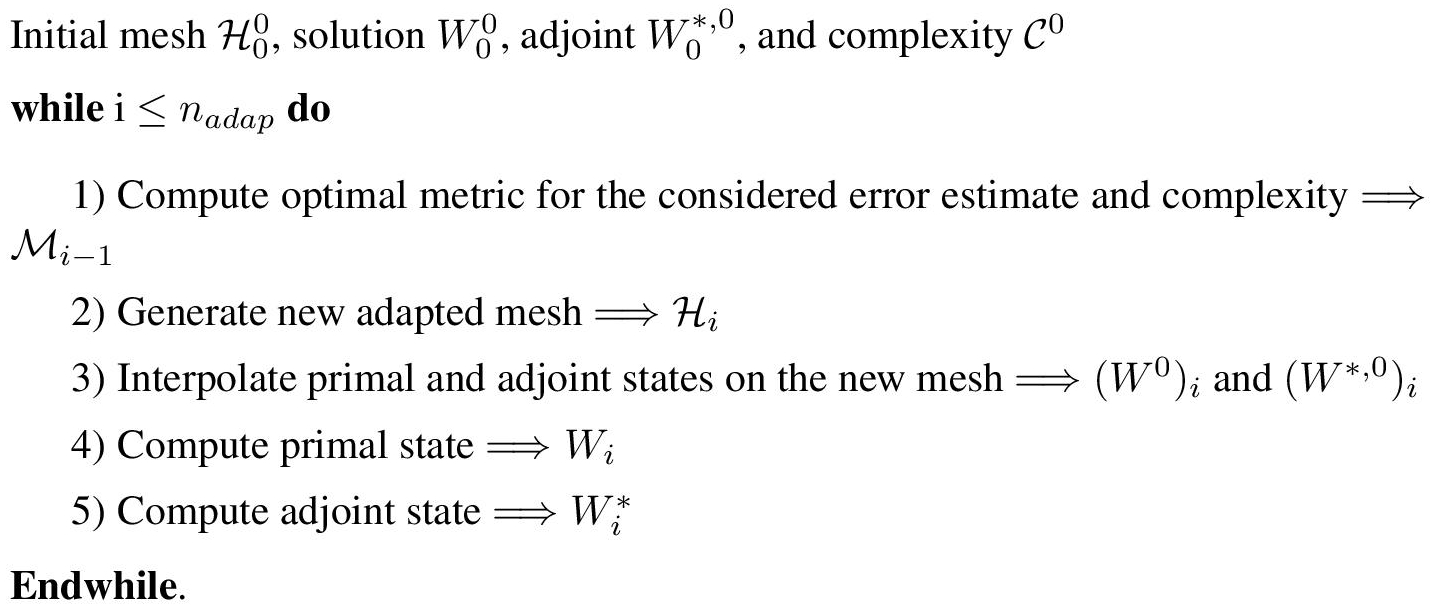
From an initial triple mesh-solution-adjoint ![]() (converged on current mesh), it is composed of the following sequences. At step i, a metric tensor field
(converged on current mesh), it is composed of the following sequences. At step i, a metric tensor field ![]() is deduced from
is deduced from ![]() because of the anisotropic error estimate. The latter is used by the adaptive mesh generator that generates a unit mesh with respect to
because of the anisotropic error estimate. The latter is used by the adaptive mesh generator that generates a unit mesh with respect to ![]() The previous solution and adjoint are then linearly interpolated on the new mesh, and iteratively converged to solution and adjoint solutions on the current mesh
The previous solution and adjoint are then linearly interpolated on the new mesh, and iteratively converged to solution and adjoint solutions on the current mesh ![]() This procedure is repeated until convergence of the couple mesh-solution.
This procedure is repeated until convergence of the couple mesh-solution.
In next section, we investigate the novelties to be introduced when dealing with the adjoint-based anisotropic error estimate. The main modifications concern the flow and adjoint solver and the remeshing stage. In this section, the following notations are used. H denotes the mesh of the domain Ωh, ∂H the mesh of the boundary Γh of Ωh, Wh is the state provided by the flow solver and j(Wh) the observed functional defined on ![]() .
.
4.5.1. Adjoint solver
As compared to Feature-based mesh adaptation, an extra step to add to the solver is the resolution of the linear system providing the adjoint state: ![]() where gh is the approximated jacobian of j(Wh) with respect to the conservative variables and
where gh is the approximated jacobian of j(Wh) with respect to the conservative variables and ![]() is the adjoint state. The state is solved with the linearized implicit pseuso-unsteady method using a spatially first-order accurate Jacobian Ah. It is described in Chapter 1 of Volume 1. We define
is the adjoint state. The state is solved with the linearized implicit pseuso-unsteady method using a spatially first-order accurate Jacobian Ah. It is described in Chapter 1 of Volume 1. We define ![]() as the adjoint of Ah. In the Wolf code, the linear systems for
as the adjoint of Ah. In the Wolf code, the linear systems for ![]() (as for Wh) is solve with the iterative GMRES method coupled with an incomplete BILU(0) preconditioner (Saad 2003). Once
(as for Wh) is solve with the iterative GMRES method coupled with an incomplete BILU(0) preconditioner (Saad 2003). Once ![]() is computed, its vertex gradient
is computed, its vertex gradient
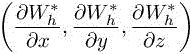
is recovered by using a L2 projection from the neighboring element-wise constant gradients (Alauzet and Loseille 2009a).
4.5.2. Optimal goal-oriented discrete metric
The continuous optimal metric discussed in section 4.4 is composed of a volume tensor field Mgo defined in Ω and a surface one ![]() defined on Γh. For the discrete case, we compute the following:
defined on Γh. For the discrete case, we compute the following:
– for each vertex x of H, the pseudo-Hessian matrix arising from the volume contribution of each component of the Euler fluxes:
where
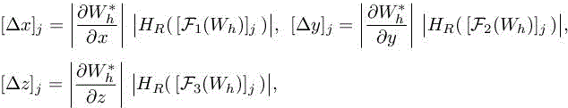
with ![]() denoting the jth component of the vector
denoting the jth component of the vector ![]() ;
;
– for each vertex x of ∂H, the pseudo-Hessian matrix arising from the surface contribution:
where n =(n1, n2, n3) is the outward normal of Γ.
HR stands for the operator that recovers numerically the second derivatives of an initial piecewise linear by element solution field. The recovery method is based on the Green formula method, described in section 5.4.3 of Volume 1. The standard L1 norm normalization is then applied independently on each metric tensor field:
Constants C and ![]() depend on the desired complexity N.
depend on the desired complexity N.
A natural synthesis between the volumic pseudo-Hessian H and the surfacic pseudo-Hessian ![]() is to define the final optimal metric as
is to define the final optimal metric as
Of course, a special decimation4 needs to be applied to match smoothly the boundary metric and the volumic one. In practice, numerical experiments (see Loseille 2008) show that the resulting functional prediction is not notably improved by accounting the boundary metric and that measured convergence order slightly degrades due to the extra vertices. A particular case is the case of a symmetric flow. Computing the complete flow leads to having no special boundary term on the symmetry plan, while computing the half flow adds a couple vertices near the symmetry plan. This tends to show that at least with slip conditions the boundary metric is not necessary5.
In the presented experiment, the surfacic terms of the adaptation criterion are neglected.
REMARK 4.1 (Non-convergence of goal-oriented formulation).– We want to emphasize that the goal-oriented formulation is designed to favor the best convergence of the prediction of the scalar functional, but it is not designed to produce the flow field convergence. This point is illustrated in next section.
4.5.3. Controlled mesh regeneration
We use Yams (Frey 2001) for the adaptation of the surface and an anisotropic extension of Gamhic (George 1999) for the volume mesh. When the surface is not adapted, we use Mmg3d (Dobrzynski and Frey 2008).
4.6. Numerical outputs
4.6.1. High-fidelity pressure prediction of an aircraft
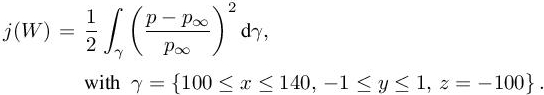
We consider the flow around a supersonic business jet (SSBJ). The code Wolf is used. The geometry provided by Dassault-Aviation is depicted in Figure 6.3 (left) of Volume 1. Flight conditions are Mach 1.6 with an angle of attack of 3◦. As for a body flying at a supersonic speed, each geometric singularity generates a shock wave having a cone shape; a multitude of conic shock waves are emitted by the aircraft geometry. They generally coalesce around the aircraft while propagating to the ground. The goal, here, is to compute accurately the pressure signature only on a plane located 100 m below the aircraft. The scope of this test case is to evaluate the ability of the adjoint to prescribe refinements only in areas that impact the observation region. The functional is given by
 [4.18]
In order to exemplify how adjoint-based mesh adaptation gives an optimal distribution of the degrees of freedom to evaluate the functional, this adaptation is compared to the Hessian-based mesh adaptation (the adaptation is done on the local Mach number and the interpolation error is controlled in L2 norm) presented in section 6.4 of Volume 1.
We apply the convergent steady fixed point Algorithm 4.1. The adaptive loop is divided into five outer steps. The complexity sequence is [10,000, 20,000, 40,000, 80,000, 160,000]. Each step is composed of six sub-iterations at constant complexity for a total of 30 adaptations. Hessian-based and adjoint-based final adapted meshes are composed of almost 800,000 vertices. They are represented in Figure 4.1 where several cuts in the final adapted meshes for the adjoint-based (top) and Hessian-based (bottom) adaptations are displayed.
For the Hessian-based adaptation, the mesh is adapted in the whole computational domain along the Mach cones and in the wake (see Figure 4.1, right). Such an anisotropic adapted mesh provides an accurate solution everywhere in the domain. But, if the aim is to only compute an accurate pressure signature on surface γ, then we clearly notice that a large amount of degrees of freedom is wasted in the upper part of the domain and in the wake where accuracy is not needed.
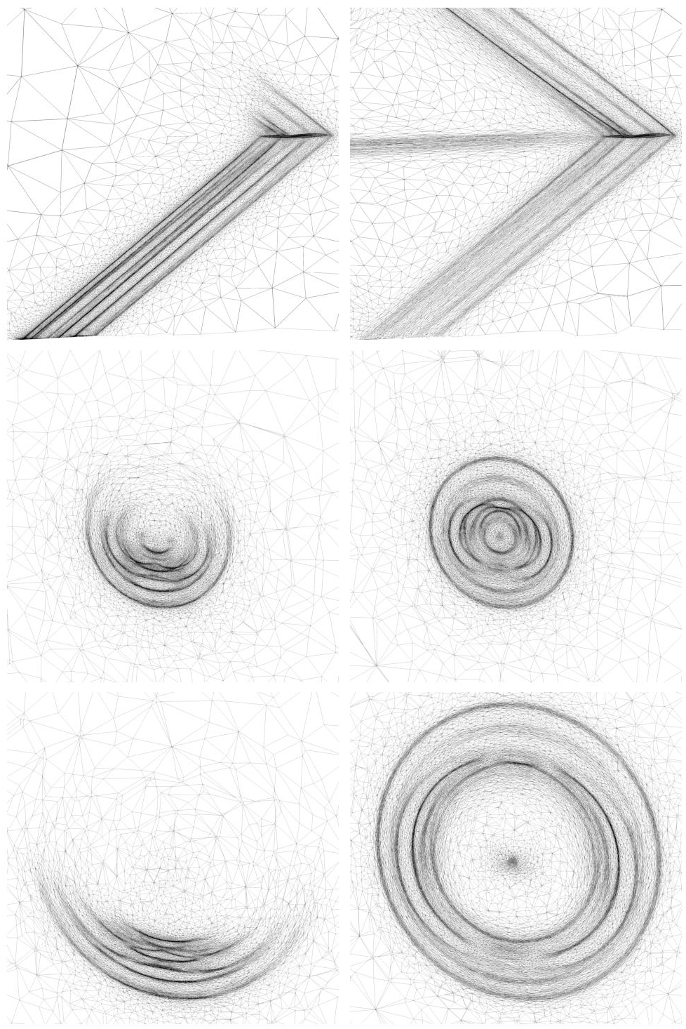
Figure 4.1. Cut planes through the final adapted meshes for the adjoint-based (left) and Hessian-based (right) methods. Top, a cut in the symmetry plane and, middle and bottom, two cuts with an increasing distance behind the aircraft orthogonal to its path
With regard to the adjoint-based adaptation, the mesh is mainly adapted below the aircraft in order to capture accurately all the shock waves that impact the observation plane (Figure 4.1, left). On the contrary, areas that do not impact the functional are ignored with the goal-oriented approach: the region over the aircraft, the wake of the SSBJ and in the region just behind the aircraft, only the lower half of the conic shock waves are refined and the angular amplitude of the refined part keeps on decreasing along with the distance to the aircraft.
Another point of interest, which is more technical, is that the Hessian-based adaptation in L2 norm prescribes a mesh size that depends on the shock intensity. A stronger shock is then more refined than a weaker one. In this simulation, shocks directly below the aircraft have a lower intensity than lateral or upper shocks emitted by the wings (see Figure 4.1, bottom). Consequently, the adapted meshes with the Hessian-based method are less accurate in regions that directly affect the observation plane. On the contrary, with the adjoint-based strategy, shocks below the aircraft are not uniformly refined. The shock waves are all the more refined as they are influent on the functional independently of their amplitudes. This has a drastic consequence on the accuracy of the observed functional (Figure 4.2).
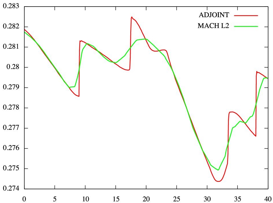
Figure 4.2. Pressure signature along x axis in the observation plane Adjoint based calculation produces very stiff shock capturing (quasi vertical segments). For a color version of this figure, see www.iste.co.uk/dervieux/meshadaptation2
As a conclusion, it is clear in the present computation that the Hessian-based adaptation gives a non-optimal result for the accuracy of the output functional. It gives an inappropriate distribution of the degrees of freedom. It is also demonstrated how the adjoint defines an optimal distribution of the degrees of freedom for the specific target. However, it is important to note that the mesh obtained with the Hessian-based strategy is somewhat optimal to evaluate globally the local Mach number field. It is also worth mentioning that the present method is completely automatic and gives an optimal result.
4.7. Conclusion
This chapter has described a method providing the anisotropic adapted mesh minimizing a first error term estimate in the approximation of a functional depending on the solution of a flow problem. This method is based on a formal a priori estimate of the functional approximation error and its minimization in an abstract continuous framework. The estimate is rather pessimistic since it does not take into account possibly compensating errors. In Chapter 5 of this volume, we discuss a more efficient estimate. With the present estimate, the goal-oriented anisotropic adaptation has been applied to the compressible Euler equations. The method has the following features:
– it produces an optimal anisotropic metric uniquely specified as the optimum of a functional and explicitly given by variational calculus from the continuous state and the adjoint state. The coupled system of the metric and the two states is the object of the discretization. This should be put in contrast with the usual process of starting from a (discrete) mesh and then improving it;
– to apply it, there is no need to choose in a more or less arbitrary way any local refinement “criterion” and no need to fix any parameter except the total number of vertices which represents the error threshold;
– mesh convergence is performed in a natural way by increasing the metric complexity at each stage of the mesh adaptation process.
The goal-oriented method is illustrated on a challenging 3D sonic boom problem. Other calculations are presented in Loseille (2008); Loseille et al. (2010a,b) and Alauzet and Loseille (2010). Numerical experiments show that the goal-oriented method enjoys at best level the advantages of Hessian-based anisotropic methods and of goal-oriented methods. As compared to the Hessian-based method, the anisotropic stretching of the meshes is not lost but even more strengthened and better distributed along shocks. Compared to traditional goal-oriented methods, the anisotropic goal-oriented method behaves like a goal-oriented method, but also naturally takes the anisotropy related to the functional into account.
4.8. Notes
This chapter revisits the study of Loseille et al. (2010b).
A paradox. O. Pironneau raised some paradox in the proposed goal-oriented adaptation algorithm. The question was: How can you adequately adapt with a criterion expressed in terms of the state and adjoint state if you do not adapt for a better state and a better adjoint?
This question is related to a particular step in the design of the mesh adaptation algorithm. Indeed, the first step in our theory is to apply a continuous metric analysis, which produces a continuous optimality system involving continuous state, continuous adjoint and continuous stationarity with respect to the metric.
In a second step, we have to discretize the whole optimality system. For this, an option could be to use a sequence of uniformly refined meshes. State and adjoint would be well refined. This option would finally produce (with a prohibitive computational cost) the optimal metric.
Once we have a good approximation of the optimal metric, we can generate unit adapted meshes based on it. By construction, these meshes are adequate for the evaluation of the functional through the evaluation of the state. In other words, the state computed with an unit mesh of the metric is a good mesh for the functional evaluation. At the same time, with this adapted mesh, the state is not well computed since only its features influencing the functional are supposed to be well computed. Adapting for a better state would then be not optimal.
Adapting for a better adjoint is a somewhat second-order approach, since it does not influence directly the quality of the approximation of the functional, but solely how close is the metric from the perfectly optimal one: formally, an ε-large deviation of the (unconstrained) quasi-optimum provokes an ε2-large deviation of the (smooth) functional value.
Lastly, an examination of [4.4] and [4.5] show the adjoint itself does not need to be accurately computed, as far as RHS of [4.4] is accurately computed. Now this RHS is equal to the RHS of [4.5], which is minimized in the present method. □
Notes
- 1 In the general case j, the derivative of j with respect to w will be taken in adjoint RHS in place of g.
- 2 Otherwise, an extra term in the error to minimize will take into account the dependency of j with respect to the mesh (i.e. to the metric).
- 3 In other words, we prefer to locally overestimate the error.
- 4 Decimation: mesh size smooth transition between a fine region and a coarse region.
- 5 Several experiments reported in Loseille et al. (2010b) have been performed with the intersection of volumic metric and surfacic metric and compared with the use of solely the volumic metric. Up to now, no computation could indicate an advantage in using the surfacic metric.