
5
Goal-Oriented Adaptation for Viscous Steady Flows
Chapter 4 introduces for the steady Euler flow model the different steps of a method for goal-oriented anisotropic adaptation. A continuous adjoint and a continuous error analysis are used for exhibiting an intermediate optimal continuous metric. The final optimal metric is solution of a (continuous) fixed point. A way of discretizing this fixed point is then introduced and constitutes the goal-oriented anisotropic mesh adaptation algorithm. This chapter extends the goal-oriented anisotropic adaptation to viscous steady compressible flows. Only the error analysis is different. With viscous terms, it is more complex. Further, due to the thin boundary layers in the flow, the efficiency of adaptation is much more influenced by the quality of the error estimate. The central principle of this kind of analysis is again to express the right-hand side of the error equation, often referred as the local error, as a function of the interpolation error of a collection of fields present in the nonlinear partial differential equations. Two approaches are considered and compared. Applications to mesh adaptive calculations of flows past airfoils and a wing-body combination are discussed.
5.1. Introduction
This chapter focuses on the building of an anisotropic goal-oriented mesh adaptation method for viscous flows. The way to derive such a method for inviscid flows was described in the previous chapter. In order to extend it to an elliptic or parabolic model, we need an adequate derivation of the error estimation when second spatial derivatives are present in the PDE. We first focus on an elliptic generic model and propose two adjoint-based a priori analyses. We then extend these analyses to the compressible Navier–Stokes system, which involves nonlinear parabolic terms. For the first a priori analysis, we demonstrate by manipulating the nonlinear viscous terms that each of them can be written as a combination of an elliptic terms (on which the above-mentioned error estimation applies) and higher-order error terms (which can be neglected). The second a priori analysis is identified as satisfying some important criteria, namely a smaller set of interpolation error restricted to the conservative variables, and as giving a more compact formulation allowing for possible compensation in errors.
The chapter is outlined as follows. Section 5.2 proposes the two a priori estimates for the Poisson problem. The two goal-oriented error estimates for the Navier–Stokes equations are given in section 5.3. Finally, section 5.4 states how the optimal discrete meshes is obtained, and section 5.5 presents an application to a high-lift flow.
5.2. Case of an elliptic problem
5.2.1. A priori finite-element analysis (first estimate)
Standard a priori estimates have been early derived in H1(Ω) (“projection property”), and in L2(Ω) (Aubin–Nitsche analysis), but only by means of inequalities. The leading term of the error is generally not exhibited, but only bounds of it are proposed in term of H2 norm of the unknown. In this section, we go a little further in order to evaluate a first term in the upper bound in the second-order terms. Let us focus on the Poisson problem set on domain ![]() :
:
Its variational form is
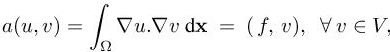
where V holds for the Sobolev space ![]()
![]() . In order to derive an a priori estimate, we assume that solution u has some extra smoothness:
. In order to derive an a priori estimate, we assume that solution u has some extra smoothness:
where ![]() is the set of functions of class C3 on
is the set of functions of class C3 on ![]() 1. Let H be a mesh of Ω made of simplices (triangles in 2D and tetrahedra in 3D): H = ⋃k Kk. Let Vh be the subspace of V of continuous functions that are P 1 on each element of the mesh:
1. Let H be a mesh of Ω made of simplices (triangles in 2D and tetrahedra in 3D): H = ⋃k Kk. Let Vh be the subspace of V of continuous functions that are P 1 on each element of the mesh:
The discrete variational problem is then defined by
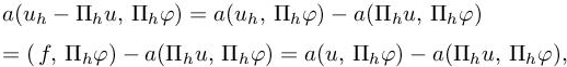
Let Πh be the linear interpolation operator Πh defined and analysed in section 4.2 of Volume 1. In a simplified goal-oriented analysis, we are interested in estimating (g, uh − u), which can be split into two components:
where we recognize in the second difference Πhu − u the interpolation error, and the first difference uh − Πhu is referred as the implicit error. Introducing the continuous and the discrete adjoint states ![]() verifying
verifying
we get
The second term of the right-hand side can be estimated without any difficulty using corollary 4.1 of Volume 1:

while it would have been a lot more complicated using the equality ![]() Analyzing the first term of the right hand-side of relation [5.5] leads to study the following term:
Analyzing the first term of the right hand-side of relation [5.5] leads to study the following term:
where φ is any sufficiently smooth function. To this end, we first express the implicit error term as a function of the interpolation error. It is useful to remark that the discrete statement is equivalently written as
Using relation [5.6] and then relation [5.2], we get
which gives2
Then we shall use the following estimate, the proof of which can be found in Belme et al. (2019):
LEMMA 5.1.– For any couple of smooth functions (u, φ), where u is not necessarily a solution of problem [5.1], we have the following bounds:

where Kd =3 in two dimensions, Kd =6 in three dimensions and ![]() holds for a majoration asymptotically valid, that is, A ≤ B + o(A) when mesh size tends to zero. Expression | ρH(φ) | holds for spectral radius of H(φ), which is the Hessian of φ, that is, the largest (in absolute value) eigenvalue of H(φ). The boundary terms BT are not used in the sequel. □
holds for a majoration asymptotically valid, that is, A ≤ B + o(A) when mesh size tends to zero. Expression | ρH(φ) | holds for spectral radius of H(φ), which is the Hessian of φ, that is, the largest (in absolute value) eigenvalue of H(φ). The boundary terms BT are not used in the sequel. □
The estimate of lemma 5.1 is successfully tested for mesh adaptation in the sequel in Chapter 6, in more detail in Brèthes and Dervieux (2016) and also compared with another estimate in Brèthes and Dervieux (2017).
5.2.2. Goal-oriented adaptation according to lemma 5.1
We keep the notations introduced in Chapter 4, and in particular, we minimize the error ![]() depending on a metric M and done in the evaluation of the scalar output j = (g, u) by discretizing the flow under study with a mesh defined by the metric M. The scalar error considered is simplified as follows:
depending on a metric M and done in the evaluation of the scalar output j = (g, u) by discretizing the flow under study with a mesh defined by the metric M. The scalar error considered is simplified as follows:
Let us define the discrete adjoint state ![]() :
:
Then
and, using [1.8],
thus
Recall that u is unknown. The second term Πhu − u, similar to the main term of the Hessian-based adaptation in section 6.2.1, can be explicitly approached in the same way, that is, introducing the continuous interpolation error of corollary 4.1 of Volume 1:

For the second Πhu − u term, we first apply lemma 5.1 and then also introduce the continuous interpolation error. We get

It is then reasonable to try to minimize the RHS of this inequality instead of the LHS. But this still involves some difficulty due to the dependency of adjoint state ![]() with respect to M. We shall further simplify our functional by freezing the adjoint state during a part of the algorithm. The idea is that when we change the parameter M, the discrete adjoint
with respect to M. We shall further simplify our functional by freezing the adjoint state during a part of the algorithm. The idea is that when we change the parameter M, the discrete adjoint ![]() is close to its (non-zero) continuous limit and is thus not much affected, in contrast to the interpolation errors
is close to its (non-zero) continuous limit and is thus not much affected, in contrast to the interpolation errors ![]() We then consider, for a given M0, the following optimum problem:
We then consider, for a given M0, the following optimum problem:

This produces an optimum:
Observing that, in the integrand, the matrix
is positive symmetric positive, we can apply the calculus of variation and get

where K1 is defined in [4.40] of corollary 4.2 of Volume 1. This solution can then be introduced in a fixed-point loop and will result in the solution

This expression is the analog of reference [4.16] derived in Chapter 4 for steady Euler flow. It permits after discretization to apply an anisotropic goal-oriented algorithm, for example, Algorithm 4.1 of this volume (the viscous version is given as Algorithm 5.2 in the sequel).
5.2.3. Goal-oriented adaptation according to a second estimate
We give now a development inspired by Michal et al. (2018a) and allowing the compensation of terms in the estimate, and therefore possibly giving a more accurate estimate than [5.8]. We define
The analysis starts as follows:
Then, integrating by parts, we pass the derivatives on the adjoint state (again neglecting boundary terms):

Then replacing FV , we get

This error estimate is a weighted sum of interpolation errors in L1-norm on the unknown and the RHS, where the weights depend on the Hessian of the adjoint state:

Similarly to the previous section, we consider, for a given M0, the following optimum problem:
This produces an optimum (with frozen adjoint):
(again an analog of reference [4.16] of section 4.4 of Chapter 4 of this volume) and completes the evaluation of the optimal metric. In this more globally linearized second estimate, we have more freedom for terms to compensate each other, thus obtaining a more accurate estimate.
We do not present in this chapter any numerical validation relying on the two above elliptic analyses, which we use as models for the Navier–Stokes applications. Chapter 6 of this volume presents such a validation for an extension of the first elliptic analysis.
5.3. Error analysis for Navier–Stokes problem
5.3.1. Mesh adaptation problem statement
We continue to assume that the purpose of the numerical problem is to evaluate the output functional j, but this time expressed through a steady Navier–Stokes system:
More precisely, let us consider the continuous W and discrete Wh solutions of the continuous [1.51] and discrete [1.55] laminar Navier–Stokes models introduced in Chapter 1 of Volume 1. The problem addressed in this chapter is to find the discrete mesh which minimizes the following functional error given a fixed number of vertices N:
where W is the solution of problem [1.51] and Wh is the solution of problem [1.55].
This section and the next ones are devoted to this error analysis and the optimal formulation of the mesh adaptation problem. Let ψ be a smooth test function of V. Let W be the solution of problem 1.51 and Wh the solution of problem [1.55], and the continuous and discrete state equation is written as
where Πhψ lies in Vh defined by relation [1.54]. We also introduce the continuous and the discrete adjoint states: W∗ and Wh∗. The continuous adjoint system related to the objective functional is written as
From functional analysis theory, a well-posed continuous adjoint system can be derived for any functional output as far as the linearized system is well posed. This, however, does not mean that any output functional leads to properly defined adjoint boundary conditions. Several works in the literature (Anderson and Venkatakrishnan 1999; Arian and Salas 1999; Bueno-Orovio et al. 2012; Castro et al. 2007) illustrate this problem and propose solutions, usually by adding auxiliary boundary terms to the Lagrangian functional. In Castro et al. (2007), it is concluded that for the compressible Navier–Stokes system, only functionals that involve the entire stress tensor at obstacle boundary are admissible. We assume here that [5.10] is well posed and gives a sufficiently smooth continuous adjoint state. The discrete adjoint system is written as
5.3.2. Linearized error system
In our error estimation problem presented in section 5.3.1, the approximation error can be decomposed into an implicit error term and an interpolation error term:
The interpolation error can be easily estimated, corollary 4.1 of Volume 1, while the implicit error is solution of a discrete system that we derive in the following. Now, we assume that Wh can be made close enough to ΠhW when h → 0 in such a way that we can write
Then, combining continuous and discrete systems, we can write similarly to relation [5.7] an equality linking implicit and interpolation errors, which is valid for all ψ:
We are then interested in the following error on the functional:
The right-hand side of the above relation is composed of the Euler term (see relation [1.55]), the Euler boundary term, the viscous term and the stabilization term. In the following, we neglect the boundary term (as in the previous analysis) and the stabilization term because of smoothness of functions W and W∗ 3. The method proposed here involves some heuristics. In particular, we assume that the interpolate of the adjoint is close to the discrete adjoint:
Therefore
5.3.3. First estimate for Navier–Stokes problem
The first a priori estimate that we propose is stated as follows:
PROPOSITION 5.1.– Let us assume that W ∈ V and ![]()
![]() . Then, we have the following error bound for h sufficiently small:
. Then, we have the following error bound for h sufficiently small:
with:
and Kd =3 in two dimensions, Kd = 6 in three dimensions, and A ≼ B holds for a majoration asymptotically valid, that is, A ≤ B + o(A) when mesh size tends to zero. Expression | ρH(φ) | holds for spectral radius of the Hessian of φ.
The proof of this proposition is very technical and is given in Belme et al. (2019). □
This main result can be written in a more convenient way to facilitate its implementation by gathering interpolation error terms on the primitive variables. We give now the 2D and the 3D re-writing of it.
COROLLARY 5.1.– Let us assume that W ∈ V and ψ ∈ V, ψ = (ψρ,ψρu1 , ψρu2 ,ψρE)T . Then, in two dimensions (Kd = 3), we have the following error bound for h sufficiently small:
with the coefficients
and the ω vector defined by
where only the last component is not zero. □
COROLLARY 5.2.– Let us assume that W ∈ V and ψ ∈ V, ψ = (ψρ, ψρu1 , ψρu2 , ψρu3 ,ψρE)T . Then, in three dimensions (Kd = 6), we have the following error bound for h sufficiently small:
with the coefficients
and the ω vector defined by
![]() . □
. □
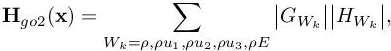
For using the estimate in a mesh adaptation loop, we seek for the optimal mesh that minimizes the above error model. It is useful to note that the error model can be written under the compact form:
In other words, the error model is a sum of interpolation errors weighted by algebraic functions.
We can reformulate the discrete mesh adaptation problem introduced in section 5.3.1 in the continuous mesh framework: find the continuous mesh Mopt which minimizes the following functional error given a fixed complexity N :
where W is the solution of problem 1.51, Wh is the solution of problem [1.55] and W∗ is the solution of problem [5.10].
The above relation is a weighted sum of interpolation errors. By introducing the following positive symmetric matrix
where |HWk | and |HSk(W)| are the absolute value of the Hessian of fields Wk and Sk(W), and using the definition of the continuous interpolation error given by corollary 4.1 of Volume 1, we can state the following error estimate on continuous mesh M =(M(x))x∈Ω:
5.3.4. Second estimate for Navier–Stokes problem
We adapt the second estimate for elliptic case (see section 5.2.3). In Michal et al. (2017, 2018a,b), this type of analysis was proposed for Navier–Stokes and has proved to be more efficient on the ONERA M6 case, among other cases, than the first estimate of previous section. While in Michal et al. (2017, 2018a,b) an approximation was made by using only the Hessian of the Mach number variable, we propose here to introduce ingredients of the first estimate in order to derive a sharper viscous goal-oriented error estimate. Moreover, this analysis can be done on the conservative variable to end-up only with five terms in the error estimation. Both inviscid and viscous fluxes are linearized with respect to the solution W and its gradients ∇W and integrating by parts (and omitting the boundary terms), we obtain
This implicit error estimate is a weighted sum of interpolation errors in L1-norm on the conservative variables where the weights depend on the gradient and the Hessian of the adjoint state and on the convective and viscous fluxes. We just have to add the interpolation error term to have the approximation error estimate:
For practical implementation, we give the expression of the weights in 3D for each conservative variable:
with
where we have
Again, we can re-use the interpolation error analysis, this time with
to obtain a second estimate:

For RANS computations, this estimate should also take into account in the estimate the turbulent closure equations. Our option here is to neglect them. The influence of turbulence modeling is then limited to accounting the variables μt and λt in the mean flow equations.
5.3.5. Optimal goal-oriented continuous mesh
Equipped with the estimate
it is possible to set the well-posed global optimization problem of finding the optimal continuous mesh Mgo minimizing continuous interpolation error Ego(M):
We seek for the optimal continuous mesh Mgo solution of problem [5.13]. In a similar way to Chapter 4 of this volume, solving the optimality conditions provides the optimal goal-oriented continuous mesh ![]() defined point-wise as follows (we recall that d is the space dimension):
defined point-wise as follows (we recall that d is the space dimension):

The corresponding optimal error is written as
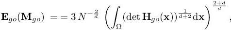
where the exponent of N illustrates the second-order accuracy of the method.
5.4. From theory to practice
The continuous mesh adaptation problem takes the form of the following continuous optimality system:
In practice, it is necessary to approximate the above three-field coupled system by the discrete optimality system:
The discrete optimality system is solved using the fixed-point mesh adaptation Algorithm 5.1. In practice, Algorithm 5.1 should be called by Algorithm 6.1 of Volume 1 for obtaining mesh-converged results.
Algorithm 5.1. Viscous goal-oriented mesh adaptation loop for steady flows
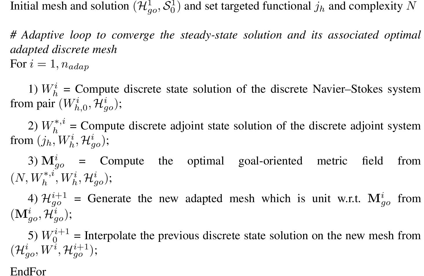
The discrete state equation is modeled with Wolf code as in section 1.2.11 of Volume 1. With regard to the adjoint state computation, the matrix of the linear system is simply the transpose of the implicit state equation matrix without the time derivative term. The right hand-side of the system is the exact differentiation with respect to state of the chosen functional (for instance, drag, lift and so on):
In particular, for viscous flows, μ and the stress tensor τ are exactly differentiated. To solve the adjoint system, we use a restarted GMRES preconditioned with SGS relaxation. Note that it is important to solve the adjoint linear system to machine precision.
5.4.1. Computation of the optimal continuous mesh
The expression of the optimal goal-oriented metric field is either given by relations [5.11]–[5.14] where algebraic functions Gk and Sk are given in corollaries 5.1 and 5.2 where ψ is replaced by the adjoint W∗, or by using section 5.3.4. This expression involves the state and the adjoint state, and their derivatives (first and second). In practice, these terms are approximated by the discrete states and a derivative recovery is applied to get gradients and Hessians. The recovery method is based on the double L2-projection formula described in Chapter 5 of Volume 1. We then obtain a discrete metric field defined at vertices of the mesh. The discrete adjoint state Wh∗ is taken to represent the adjoint state W∗. The gradient of the adjoint state ∇W∗ is replaced by ![]() where ∇R stands for the operator that recovers numerically the first derivatives of an initial piecewise linear solution field. The Hessian is obtained by applying the recovery operator two times: HR = ∇R ◦ ∇R. Then, | ρH(W∗)| is obtained from
where ∇R stands for the operator that recovers numerically the first derivatives of an initial piecewise linear solution field. The Hessian is obtained by applying the recovery operator two times: HR = ∇R ◦ ∇R. Then, | ρH(W∗)| is obtained from ![]() which is evaluated by computing the maximal (in absolute value) eigenvalue of HR(Wh∗). Similarly, the discrete state Wh is taken to represent the state W and to compute the Euler fluxes, velocity components and temperature (i.e. each term Sk(W) is replaced by Sk(Wh)). The Hessians of the Sk(Wh) are obtained using the recovery operator HR and the absolute values of the Hessians are computed by taking the absolute values of the eigenvalues.
which is evaluated by computing the maximal (in absolute value) eigenvalue of HR(Wh∗). Similarly, the discrete state Wh is taken to represent the state W and to compute the Euler fluxes, velocity components and temperature (i.e. each term Sk(W) is replaced by Sk(Wh)). The Hessians of the Sk(Wh) are obtained using the recovery operator HR and the absolute values of the Hessians are computed by taking the absolute values of the eigenvalues.
5.5. An example of application to a turbulent flow
The goal-oriented mesh adaptation has been applied in Alauzet and Frazza (2020) to the high-lift version of the NASA CRM (HL-CRM) geometry used for the 3rd AIAA CFD High Lift Prediction Workshop (Rumsey et al. 2018) (HLPW3). A preliminary series of computations of this case showed that the first laminar estimate did not give good adaptation. We have retained in this chapter what appeared to be the two best error estimates:
– the feature-based error estimate controlling the interpolation of the local Mach number in L4-norm;
– the goal-oriented error estimate given by relations [5.11]–[5.14].
For each error estimate:
– at most nadap = 20 mesh adaptation iterations are performed at each fixed complexity and for the convergence study we consider five complexities (320,000; 640,000; 1,280,000; 2,560,000; 5,120,000);
– the convergence study is started with an initial mesh composed of 229,263 vertices, It is a very coarse inviscid mesh without any boundary layer or any specific refinement for viscous flows, in other word no meshing guidelines, thus very easy and quick to generate. Starting from this coarse and clearly unresolved mesh aims at illustrating the non-dependency of the mesh-adaptive solution platform to the initial mesh;
– for the given complexities, the final adapted meshes involve between 0.7M vertices and 10.2M vertices.
In Alauzet and Frazza (2020), the results obtained with the mesh-adaptive solution platform are compared to all the results obtained during the workshop and this allows to observe a similar quality of prediction between the workshop fine mesh results (205M vertices) and the mesh adaptive calculation with 10.2M vertices adapted mesh. The feature-based option is clearly less efficient than the goal-oriented option in this case but it produces similar results to the best practice meshes of workshop, with seven times less vertices.
For mesh convergence, we have combined Algorithm 5.1 with Algorithm 6.1 of Volume 1. The convergence of the lift value for the viscous goal-oriented error estimate throughout the whole mesh-convergence analysis is shown in Figure 5.1 (left). It shows the evolution of the lift for each computation in red (i.e. each adaptation at each complexity) and the final retained value obtained for each complexity in blue. We note that a lot is done on coarse adapted meshes (which is cheap), while the minimum number of iterations is done on the finer adapted meshes. Again, converging on coarse meshes is advantageous and enables early capturing of the solution. Figure 5.1 (right) compares the convergence of the lift for the solution mesh-adaptive platform (red and blue lines) with respect to all workshop entries (green lines). This again emphasizes the early capturing of the lift value on coarse adapted meshes in comparison to the meshes used for the workshop.
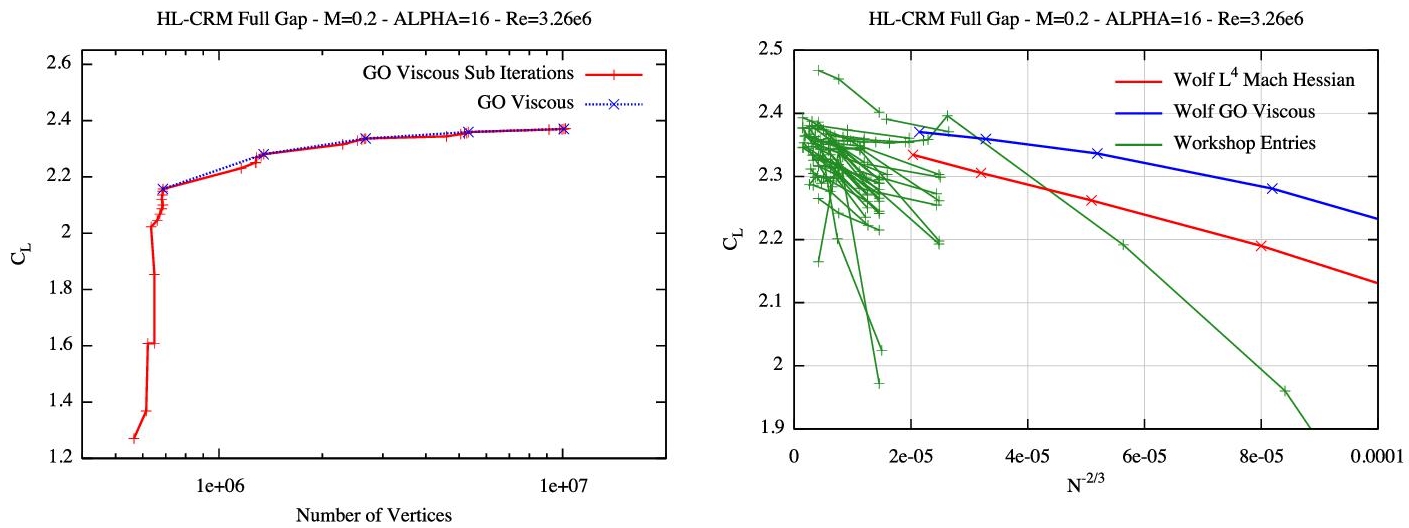
Figure 5.1. HL-CRM 16◦ case. Left: Convergence history of the total lift value CL for the viscous goal-oriented error estimate throughout the whole mesh-convergence analysis. In red, the convergence of the total lift at each complexity and, in blue, the global convergence of the total lift by retaining the final lift value for each complexity. Right: Convergence of the total lift for the solution mesh-adaptive platform with the feature-based error estimate (red line) and the viscous goal-oriented error estimate (blue line) with respect to all workshop entries (green lines)
Now, we illustrate in a series of figures the favorable behavior of adaptation for capturing some important non-trivial details in the flow. The 5M vertices adapted mesh obtained with the viscous goal-oriented error estimate is used. We also show the local Mach number of the solution for each of these cuts to display all the high-lift flow features that are automatically capture by the mesh-adaptive solution process. Figure 5.2 displays a global view of the HL-CRM with a cut plane at x = 50 to emphasize the wake refinement. The medium and fine meshes of the workshop are refined isotropically in a large rectangular region hoping that the wake will be there for all angles of attack. The adapted mesh focuses only in the current wake and refine that region appropriately and anisotropically. For instance, we can clearly see the refinement of the four tip vortices coming from the main wing and the two flaps. Figures 5.3 and 5.4 exhibit close-up views of the slat and the flap for the cut plane y = 15.5. We observe that the adapted mesh focuses in the boundary layer which is very thin, the wakes of the slat and main wing that create shear layers, the wake – boundary layer merging and the flow separation over the flap, and also the separated cove flows. It is evident that meshing guidelines ask for a large number of layers in the boundary layer mesh to have some refinement far from the body in order to capture some of the shear layer. But, a shear layer located further above the body will render inefficient that strategy. Figures 5.5 and 5.6 show two details of the geometry that may impact the overall flow: the tip vortex emitted by the slat and the gap between the two flaps. First, in Figure 5.5, we observe that the adapted mesh refines a lot more the surface mesh and this mesh is highly anisotropic. Moreover, ridges of the geometry are a lot more refined because they can be at the intersection of two boundary layers or sources of detached vortices. We can also see in the adapted mesh and in the solution the wing tip vortex of the slat that interacts with the boundary layer of the main wing and detaches the flow there. Similarly, in Figure 5.6, the vortex that runs over the gap and that completely detaches the flow in that region and its interactions with the shear layers is accurately captured.
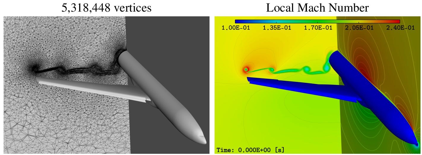
Figure 5.2. HL-CRM 16◦case. Cut plane x = 50. The 5M vertices adapted mesh obtained with the viscous goal-oriented error estimate (left) and the associated local Mach number solution (right). For a color version of this figure, see www.iste.co.uk/dervieux/ meshadaptation2
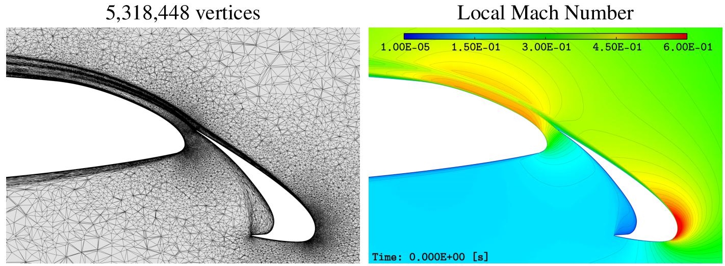
Figure 5.3. HL-CRM 16◦case. Cut plane y = 15.5 (near the flap). The 5M vertices adapted mesh obtained with the viscous goal-oriented error estimate (left) and the associated local Mach number solution (right). For a color version of this figure, see www.iste.co.uk/dervieux/meshadaptation2
In conclusion, the more complex the geometry the more efficient should be the adaptive process as it able to automatically and accurately capture all the physical features associated with these geometry details, details which are very hard to mesh accurately with classical mesh generation methods.
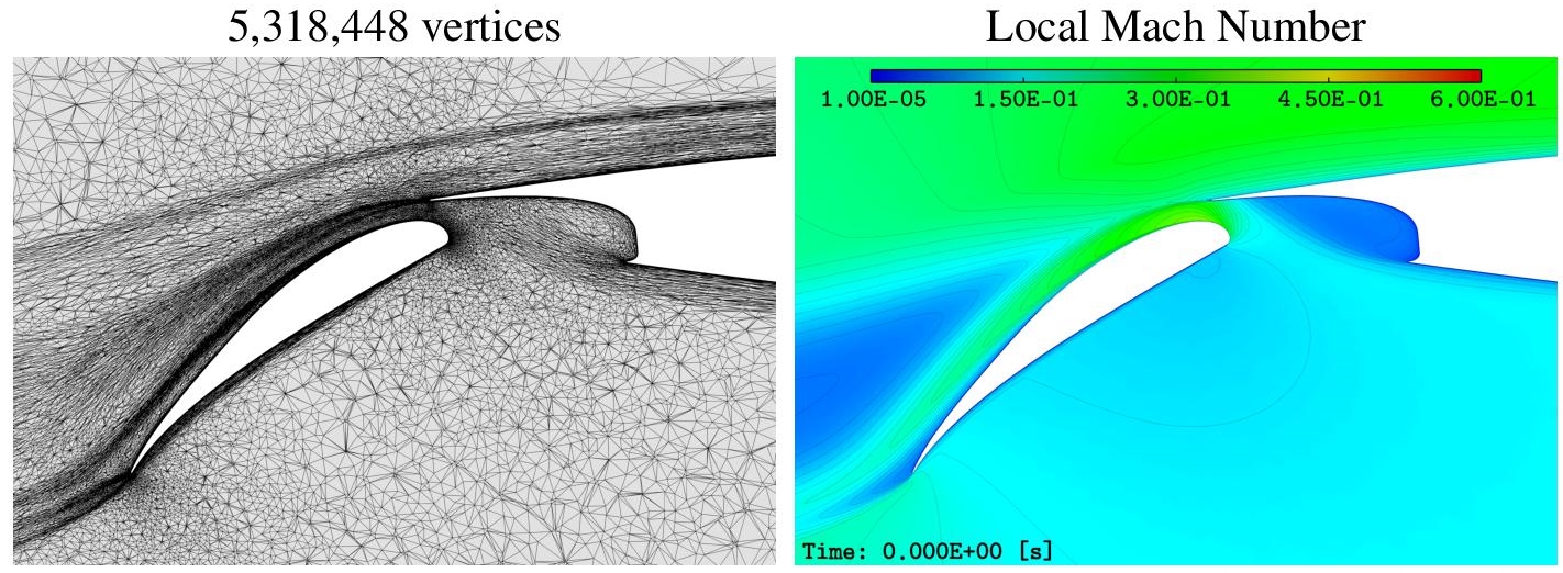
Figure 5.4. HL-CRM 16◦case. Cut plane y = 15.5 (near the slat). The 5M vertices adapted mesh obtained with the viscous goal-oriented error estimate (left) and the associated local Mach number solution (right). For a color version of this figure, see www.iste.co.uk/dervieux/meshadaptation2
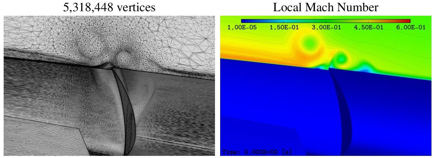
Figure 5.5. HL-CRM 16◦case. Cut plane in the region where the slat tip vortex interacts with the main wing. The 5M vertices adapted mesh obtained with the viscous goal-oriented error estimate (left) and the associated local Mach number solution (right). For a color version of this figure, see www.iste.co.uk/dervieux/meshadaptation2
5.6. Conclusion
This chapter focuses on the extension to Navier–Stokes of the goal-oriented method developped for Euler flow in the previous chapter. We have developed a cautious error analysis from the Euler one. But this analysis neglects the event of term compensation. Beside this, we have described a second goal-oriented analysis applying directly the linearization of the Navier–Stokes equations. These two goal-oriented options are supposed to produce a better convergence than the third, less sophisticated, Lp feature-based adaptation.
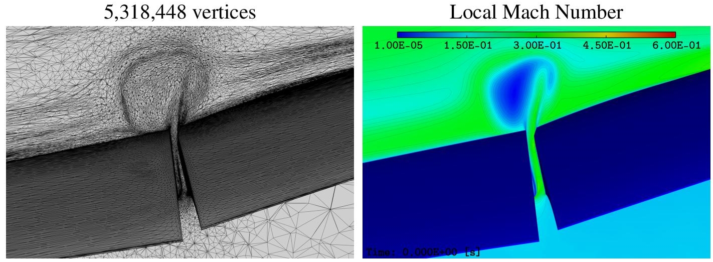
Figure 5.6. HL-CRM 16◦case. Cut plane x = 38 (near the gap between the flaps). The 5M vertices adapted mesh obtained with the viscous goal-oriented error estimate (left) and the associated local Mach number solution (right). For a color version of this figure, see www.iste.co.uk/dervieux/meshadaptation2
The three corresponding fixed point algorithms have been inserted in the mesh-convergent loop. This loop is essential for the evaluation of the efficiency of a mesh adaptation method. It appeared that the first – analysis-based – goal-oriented approach, although producing second-order convergence for Euler flows, was in our experiments unable to second-order converge with median size meshes.
In the proposed numerical illustration, the L4 feature-based and the linearized goal-oriented error estimates are compared on a high-lift workshop case. The viscous goal-oriented error estimate is clearly superior to the feature-based error estimate. Thus, it is a better choice if the adjoint state is available. With regard to the accuracy of the obtained results with the mesh adaptation process, the benefits are clear using the goal-oriented error estimate. The lift prediction agrees with the ones obtained during the workshop on the x-fine meshes composed of 206M vertices, but here the mesh size is between 5M and 10M vertices to reach that accuracy, that is, the size of the workshop coarse mesh! For the feature-based error estimate, the prediction is a bit lower and corresponds to the prediction on the fine workshop mesh (70M vertices). It will need one more level of complexity to see if it reaches the x-fine mesh prediction (note that in 2D all error estimates converge toward the same answer). In conclusion, anisotropic mesh adaptation is able to provide accurate high-lift prediction on meshes with a size similar to the coarse mesh used during the workshop. It also captures accurately all flow features and importantly all flow features that are created by geometric details. Thus, the more complex the geometry, the more efficient the adaptative process should be.
5.7. Notes
A preliminary formulation of the elliptic analysis was given in Belme (2011) and more complete derivation and extension to laminar Navier–Stokes is presented in Belme et al. (2019).
The 3D computations are presented in more details in Alauzet and Frazza (2020).
Other works. Anisotropic error estimates for elliptic models have been studied by several authors and, in particular, in Formaggia and Perotto (2001, 2003); Formaggia et al. (2004).
Acknowledgments. The work reported here was partially supported by funding from The Boeing Company with technical monitor Todd Michal. It was also partially supported by funding from Safran Tech with technical monitors Frédéric Feyel and Vincent Brunet.