
7
Goal-Oriented Adaptation for Unsteady Flows
Chapter 2 of this volume presents a transient fixed-point (TFP) multi-scale algorithm for the adaptation of mesh to an unsteady flow. Chapter 4 of this volume presents a fully anisotropic goal-oriented (GO) mesh adaptation technique for a steady flow, which uses an adjoint state and allows to define the best mesh for the most accurate evaluation of a given scalar output. The present chapter addresses the extension to unsteady flows of the GO method. Its rationale is to combine the GO of Chapter 4 of this volume with the TFP advances of Chapter 2 of this volume. However, the resulting GO-TFP has to be global in time, that is, the whole time interval needs to be computed before improved meshes are derived. Examples of applications concerns unsteady Euler flows.
7.1. Introduction
In this chapter, we define an extension of the feature-based TFP introduced in Chapter 2 of this volume to a GO formulation. To this end, several methodological issues need to be addressed. First, an error analysis based on the so-called state and adjoint systems is developed in order to set an unsteady mesh optimization problem. Second, as a necessary adaptation of the method introduced in Chapter 2, we define a global transient fixed-point (GTFP) algorithm for solving the coupled system formed, this time of three fields, the unsteady state, the unsteady adjoint state and the adapted meshes. By “global” we mean that mesh is not adapted successively time interval after time interval, but after the computation of the whole physical time of the simulation. This algorithm will be analyzed a priori and its convergence rate to the continuous solution optimized. Third, at the computer algorithmic level, it is also necessary to master the computational (memory and time) cost of the new system, which couples a time-forward state, a time-backward adjoint and a mesh update based on metric statistics over the time interval.
This chapter starts with a formal description (section 7.2) of the unsteady error analysis in its most general expression, then (section 7.3) the application to unsteady compressible Euler flows is presented. In section 7.4, the optimal adjoint-based metric is defined and all its relative issues, then section 7.5 is dedicated to strategies for mesh convergence and algorithm optimization. In section 7.6, the GTFP mesh adaptation algorithm is presented. This chapter is concluded with numerical illustrations with blast wave and acoustic wave propagation.
7.2. Formal error analysis
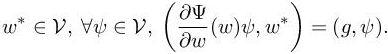
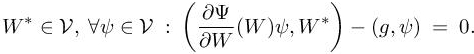
Let us introduce an unsteady system of PDEs in its variational formulation:
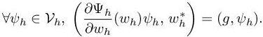
Here, the space V is made up of space–time functions, being a set of sufficiently smooth functions defined on .Ω×]0, T[, Ω being a spatial domain. The associated discrete variational formulation is written as
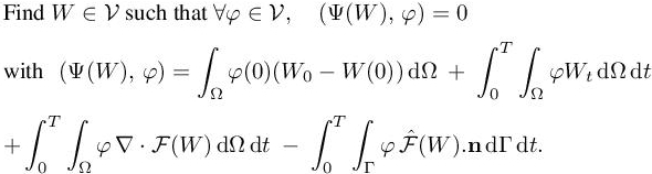
where Vh is a subspace of V. For a solution w of state system [7.1], we define a space–time functional output as
where (g, w) holds for the following rather general functional output formulation:
where gΩ, gT and gΓ are assumed to be sufficiently regular functions. We introduce the continuous adjoint w∗, solution of the following system:
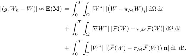
The objective here is to estimate the following approximation error committed on the functional
where w and wh are, respectively, solutions of [7.1] and [7.2]. Using the fact that Vh ⊂ V, the following error estimates for the unknown can be written as
It is then useful to choose the test function φh as the discrete adjoint state, φh = wh∗ , which is the solution of
We assume that wh∗ is close to the continuous adjoint state w∗. The same formal development as in Chapter 4 of this volume leads to the following a priori formal estimate:
The next section is devoted to the application of estimator [7.8] to the unsteady Euler model.
7.3. Unsteady Euler models
7.3.1. Continuous state system and finite volume formulation
7.3.1.1. Continuous state system
The 3D unsteady compressible Euler equations are set in the computational space– time domain Q = Ω × [0, T], where T is the (positive) maximal time and ![]() is the spatial domain. In order to easily use the usual local interpolator Πh, we define our working functional space as
is the spatial domain. In order to easily use the usual local interpolator Πh, we define our working functional space as ![]() , that is the set of measurable functions that are continuous with square integrable gradient. We formulate the Euler model in a compact manner with a variational formulation in the functional space
, that is the set of measurable functions that are continuous with square integrable gradient. We formulate the Euler model in a compact manner with a variational formulation in the functional space ![]()
Here, W is the vector of conservative flow variables and ![]() is the usual Euler flux (see [1.1] and [1.2] in Volume 1). Functions φ and W have five components, and therefore the product φW holds for
is the usual Euler flux (see [1.1] and [1.2] in Volume 1). Functions φ and W have five components, and therefore the product φW holds for ![]() . We have denoted by Γ the boundary of the computational domain Ω, n is the outward normal to
. We have denoted by Γ the boundary of the computational domain Ω, n is the outward normal to ![]() for any x in Ω, W0 the initial condition and the boundary flux
for any x in Ω, W0 the initial condition and the boundary flux ![]() contains the different boundary conditions, which involve inflow, outflow and slip boundary conditions.
contains the different boundary conditions, which involve inflow, outflow and slip boundary conditions.
7.3.1.2. Discrete state system
We first consider a spatially semi-discrete model, derived from Chapter 1 of Volume 1. We reformulate it under the form of a finite element variational formulation, this time in the unsteady context. We assume that Ω is covered by a finite-element partition in simplicial elements denoted as K. The mesh, denoted by H, is the set of the elements. Let us introduce the following approximation space:
Let Πh be the usual P1 projector:
We extend it to time-dependent functions:
The weak discrete formulation is written as follows:
with ![]() The Dh term accounts for the numerical diffusion. It involves the difference between the Galerkin central-differences approximation and the second-order Godunov approximation of Chapter 1 of Volume 1. Far from singularities, the Dh term is a third-order term with respect to the mesh size, which we do not take into account in the adaptation analysis. For shocked fields, monotonicity limiters produce first-order terms, but as in previous chapters, we let the formally second-order Hessian estimate concentrate nodes in the shocks. As concerns time discretization, we consider the following explicit RK1 time integration:
The Dh term accounts for the numerical diffusion. It involves the difference between the Galerkin central-differences approximation and the second-order Godunov approximation of Chapter 1 of Volume 1. Far from singularities, the Dh term is a third-order term with respect to the mesh size, which we do not take into account in the adaptation analysis. For shocked fields, monotonicity limiters produce first-order terms, but as in previous chapters, we let the formally second-order Hessian estimate concentrate nodes in the shocks. As concerns time discretization, we consider the following explicit RK1 time integration:

The time-dependent functional is discretized as follows:
7.3.2. Continuous adjoint system and discretization
7.3.2.1. Continuous adjoint system
We refer here to the continuous adjoint system [7.5] introduced previously:
We recall that (g, ψ) is defined by [7.4]. Replacing Ψ(W) by its definition [7.9] and integrating by parts, we get
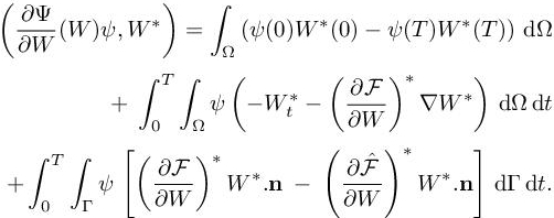
Consequently, the continuous adjoint state W∗ must be such that
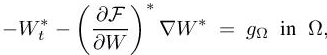
with the associated adjoint boundary conditions
and the adjoint state final condition
The adjoint Euler equations is a system of advection equations, where the temporal integration goes backwards, that is, in the opposite direction of usual time. Thus, when solving the unsteady adjoint system, we start at the end of the flow run and progress back until reaching the start time.
7.3.2.2. Discrete adjoint system
Although any consistent approximation of the continuous adjoint system could be built by discretizing [7.13], we choose the option to build the discrete adjoint system from the discrete state system defined by [7.10], [7.10] in order to be closer to the true error from which the continuous model is derived. For the sake of simplicity, we restrict to the case gT = 0 for the functional output defined by [7.4]. The problem of minimizing the error committed on the target functional j(Wh) = (g, Wh), subject to the Euler system [7.10], can be transformed into an unconstrained problem for the following Lagrangian functional:
where ![]() are the N vectors of the Lagrange multipliers (which are the time-dependent adjoint states). The conditions for an extremum are
are the N vectors of the Lagrange multipliers (which are the time-dependent adjoint states). The conditions for an extremum are
The first condition is clearly verified from [7.10]. Thus, the Lagrangian multipliers ![]() must be chosen such that the second condition of extrema is verified. This provides the unsteady discrete adjoint system
must be chosen such that the second condition of extrema is verified. This provides the unsteady discrete adjoint system
or equivalently, the semi-discrete unsteady adjoint model reads
with
As the adjoint system runs in reverse time, the first expression in the adjoint system [7.14] is referred to as adjoint “initialization”.
7.3.2.3. The memory requirement issue
Computing ![]() at time tn−1 requires the knowledge of state
at time tn−1 requires the knowledge of state ![]() and adjoint state
and adjoint state ![]() . Therefore, the knowledge of all states
. Therefore, the knowledge of all states ![]() is needed to compute backward the adjoint state from time T to 0 (Figure 7.1), which involves
is needed to compute backward the adjoint state from time T to 0 (Figure 7.1), which involves
large memory storage effort. For instance, if we consider a 3D simulation with a mesh composed of 1 million vertices, then we need to store at each iteration 5 millions solution data (we have five conservative variables). If we perform 1,000 iterations, then the memory effort to store all states is 37.25 Gb for double-type data storage (or 18.62 for float-type data storage). Two strategies are employed to reduce importantly this drawback: checkpointing and interpolation. The memory effort can be reduced by out-of-core storage of checkpoints as shown in Figure 7.2. First the state-simulation is performed to store checkpoints. Second, when computing backward the adjoint, we first recompute all states from the checkpoint and store them in memory and then we compute the unsteady adjoint until the checkpoint physical time. Therefore, with this method, the state W storage only concerns checkpoints and the timesteps inside the current checkpoint interval, with the cost of a double computation. The second strategy consists of storing solution states in memory only every m solver iterations. When the unsteady adjoint is solved, solution states between two savings are linearly interpolated. This second method leads to a loss of accuracy for the unsteady adjoint computation.We then adopt and recommend the checkpointing option.
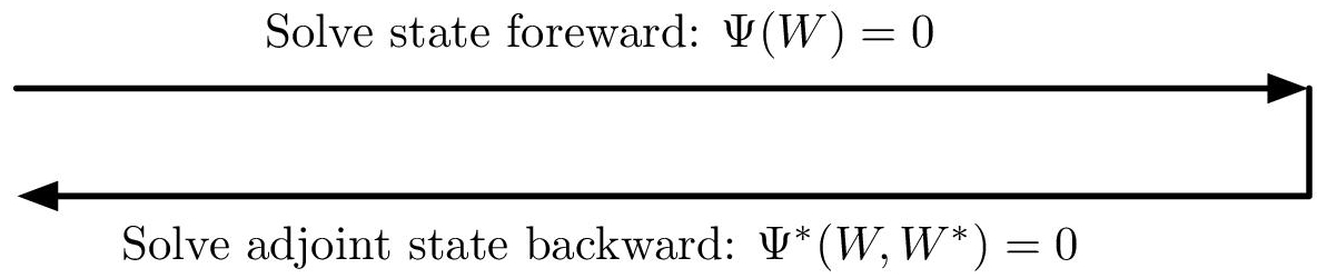
Figure 7.1. Memory issue for computing an unsteay adjoint. When state equation, going forward in time, is nonlinear, the adjoint equation, going backward in time cannot be solved without the knowledge of the state W
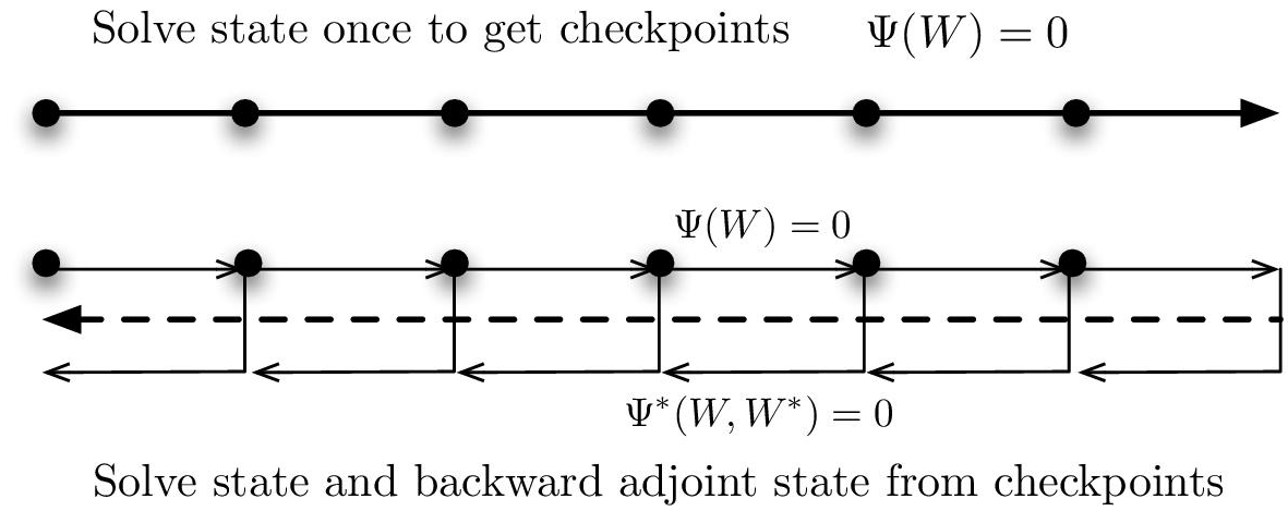
Figure 7.2. The memory issue for computing an unsteady adjoint is solved by checkpointing. On each checkpoint interval, state W is forward recomputed from a stored value at beginning of the interval. These recomputed values permit the backward advancing of the adjoint through the checkpoint interval
7.3.3. Impact of the adjoint: numerical example
Before going more deeply in the error model, we would like to emphasize how strongly the use of an adjoint may impact the density distribution of adapted meshes. The simulation of a blast in a 2D geometry representing a city is performed (see Figure 7.3). A blast-like initialization Wblast = (10, 0, 0, 250) in ambient air Wair =(1, 0, 0, 2.5) is considered in a small region of the computational domain. We perform a forward/backward computation on a uniform mesh of 22,574 vertices and 44,415 triangles. Output functional of interest j is the quadratic deviation from ambient pressure on target surface S, which is a part of the higher building roof (Figure 7.3):
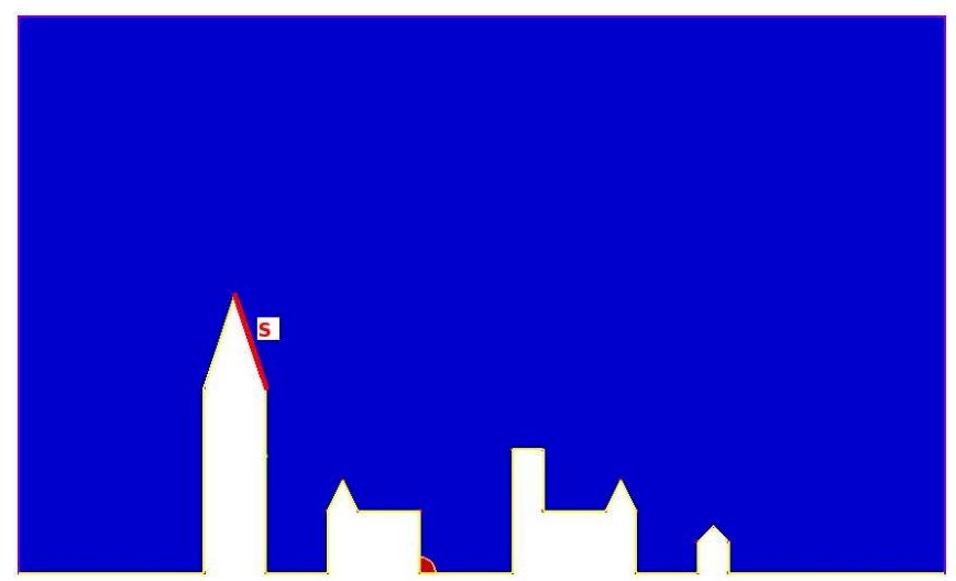
Figure 7.3. Initial blast solution (about center of bottom) and location of target surface S. For a color version of this figure, see www.iste.co.uk/dervieux/meshadaptation2
Figure 7.4 plots the density isolines of the flow at different times showing several shock waves traveling throughout the computational domain. Figure 7.5 depicts the associated density adjoint state progressing backward in time. The same a-dimensional physical time is considered for both figures.
The simulation points out the ability of the adjoint to automatically provide the sensitivity of the flow field on the functional. Early in the simulation (top left picture), many information are captured where adjoint is non-zero. We notice that shock waves which will directly impact the targeted surface are clearly detected by the adjoint, but also shocks waves reflected by the left building which will be redirected toward surface S. At the middle of the simulation, the adjoint neglects waves that are traveling in the direction opposite to S and also waves that will not impact surface S before final time T since they will not have an influence on the cost functional. While getting closer to final time T (bottom right picture), the adjoint only focuses on the last waves that will impact surface S and ignores the rest of the flow.
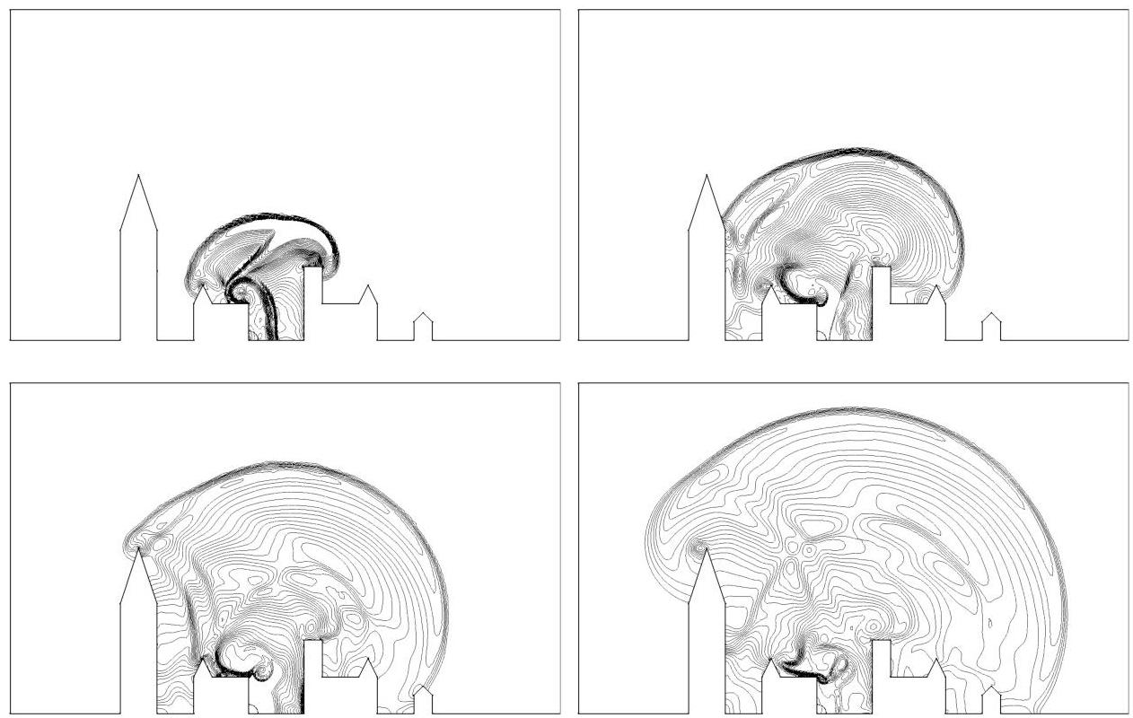
Figure 7.4. 2D city blast solution state evolution. From left to right and top to bottom, snapshot of the density isolines at a-dimensional time 1.2, 2.25, 3.3 and 4.35
7.4. Optimal unsteady adjoint-based metric
7.4.1. Error analysis for the unsteady Euler model
In estimation [7.8], operators Ψ and Ψh are now replaced by their expressions given by relations [7.9] and [7.10]. In Chapter 4 of this volume, dealing with the steady case, it is observed that even for shocked flows, it is interesting to neglect the numerical viscosity term. We follow again this option. We also discard for simplicity the error committed when imposing approximatively the initial condition. We finally get the following error model:
 [7.15]
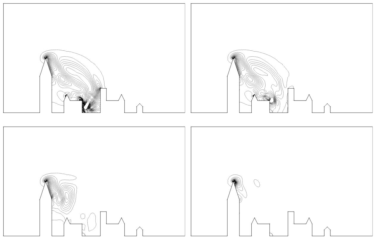
Figure 7.5. 2D city blast adjoint state evolution. From left to right and top to bottom, snapshot of the adjoint-density isolines at a-dimensional time 1.2, 2.25, 3.3 and 4.35
Integrating by parts leads to
with ![]() We observe that this estimate of δj is expressed in terms of interpolation errors of the Euler fluxes and of the time derivative weighted by continuous functions W∗ and ∇W∗.
We observe that this estimate of δj is expressed in terms of interpolation errors of the Euler fluxes and of the time derivative weighted by continuous functions W∗ and ∇W∗.
7.4.1.1. Error bound with a safety principle
The integrands in error estimation [7.16] contain positive and negative parts, which can compensate for some particular meshes. It is preferred here to not rely on these possibly parasitic effects and to (hopefully slightly) overestimate the error1. To this end, all integrands are bounded by their absolute values:

7.4.2. Continuous error model
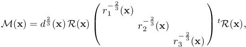
According to the continuous mesh framework, introduced in Chapter 3, a continuous mesh of computational domain Ω is identified to a Riemannian metric field ![]() and the diagonalization of M(x):
and the diagonalization of M(x):
with same notations as in Chapter 3. Given a smooth function u, to each unit mesh H with respect to M corresponds a local interpolation error |u − Πu|. In section 4.2 of Chapter 3 of Volume 1, it is shown that all these interpolation errors are well represented by the so-called continuous interpolation error related to M, which is expressed locally in terms of the Hessian Hu of u as follows:
where |Hu| is deduced from Hu by taking the absolute values of its eigenvalues and where time-dependency notations have been added for use in next sections. Working in this framework enables us to write estimate [7.17] in a continuous form:
We observe that the third term introduce a dependency of the error with respect to the boundary surface mesh. As in Chapter 4 of this volume, we discard this term.
Then, introducing the continuous interpolation error, we can write the simplified error model as follows:
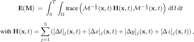
in which
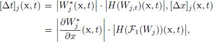
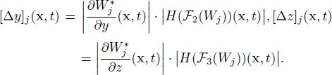
Here, ![]() denotes the jth component of the adjoint vector
denotes the jth component of the adjoint vector ![]() is the Hessian of the jth component of the vector Fi(W) and H(Wj,t) is the Hessian of the jth component of the time derivative of W. The mesh optimization problem is written as follows:
is the Hessian of the jth component of the vector Fi(W) and H(Wj,t) is the Hessian of the jth component of the time derivative of W. The mesh optimization problem is written as follows:
under the space-time complexity constraint:
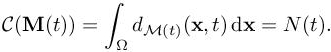
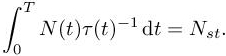
where Nst is the total space–time (st) prescribed complexity, modeling the total space– time number of nodes. In this unsteady context, the total space–time (st) complexity Cst(M) is a time integral of spatial mesh complexity weighted by the inverse time step:
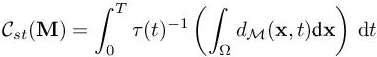
where τ(t) is the time step used at time t of interval [0,T].
7.4.3. Spatial minimization for a fixed t
Let us assume that at time t, we seek for the optimal continuous mesh Mgo(t) that minimizes the instantaneous error, that is, the spatial error for a fixed time t:
under the constraint that the number of vertices is prescribed to
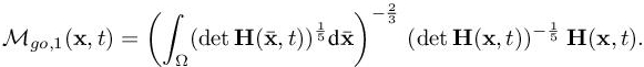
Similarly to section 4.4 of Chapter 4 of this volume, solving the optimality conditions provides the optimal goal-oriented (“GO”) instantaneous continuous mesh Mgo(t) =(Mgo(x,t))x∈Ω at time t defined by
where Mgo,1 is the optimum for C(M(t)) = 1:
The corresponding optimal instantaneous error at time t is written as:
 [7.30]
For the sequel of this chapter, we denote: ![]() .
.
7.4.4. Temporal minimization
To complete the resolution of optimization problem [7.24–7.25], we perform a temporal minimization in order to get the optimal space–time continuous mesh. In other words, we need to find the optimal time law t ⟼ N(t) for the instantaneous mesh size. First, we consider the simpler case where the time step τ is specified by the user as a function of time t ⟼ τ(t). Second, we deal with the case of an explicit time advancing solver subject to Courant time step condition.
7.4.4.1. Temporal minimization for specified τ
Let us consider the case where the time step τ is specified by a function of time t ⟼ τ(t). After the spatial optimization, the space–time error is written as
and we aim at minimizing it under the following space–time complexity constraint:
In other words, we concentrate on seeking for the optimal distribution of N(t) when the space–time total number of nodes Nst is prescribed. Let us apply the one-to-one change in variables:
Then, our temporal optimization problem becomes

The solution of this problem is given by
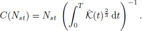
Here, the constant C(Nst) can be obtained by introducing the above expression in space–time complexity constraint [7.32], leading to
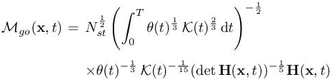
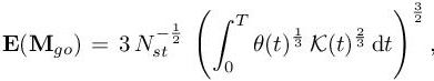
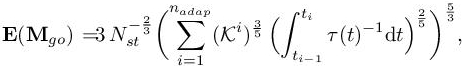
which completes the description of the optimal space–time metric for a prescribed time step. Using relation [7.28], the analytic expression of the optimal space–time GO metric Mgo is written as
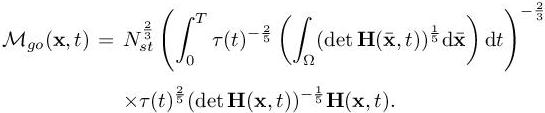
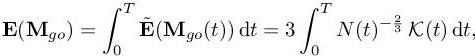
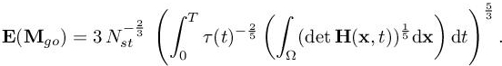
We get the following optimal error:
LEMMA 7.1.–
7.4.4.2. Temporal minimization for explicit time advancing
In the case of an explicit time advancing subject to a Courant condition, we get a more complex context, since time step strongly depends on the smallest mesh size. We restrict to the case of smooth data and solution. We still seek for the optimal continuous mesh that minimizes space–time error [7.31] under complexity constraint [7.32]. Let Δxmin,1(t) = minx mini hi(x) be the smallest mesh size of Mgo,1(t). Since the metric definition [7.18] is homogeneous with the inverse square of mesh size, we deduce the smallest mesh size of Mgo(t) from [7.28]:
where Δxmin,1(t) is independent of the mesh complexity. A way to write the Courant condition for time advancing is to define the time step τ(t) by
where c(t) is the maximal wave speed over the domain at time t. Again, we search for the optimal distribution of N(t) when the space–time complexity Nst is prescribed (see equation [7.32]), with
We choose to apply the one-to-one change in variables:
Therefore, the corresponding space–time approximation error over the simulation time interval and space–time complexity reduces to
This optimization problem has for its solution:
and by considering the space–time complexity constraint relation we deduce
Using the definitions of ![]() and
and ![]() in the above relations, we get
in the above relations, we get
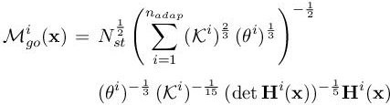
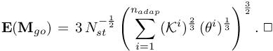
Consequently, after some simplifications, we obtain the following expression of the optimal space–time GO continuous mesh Mgo and error:
LEMMA 7.2.–
where θ(t) =c(t) (Δxmin,1(t))−1 and  . □
. □
7.4.5. Temporal minimization for time sub-intervals
The previous analysis provides the optimal size of the adapted meshes for each computational time level. Hence, this analysis requires the mesh to be adapted at each flow solver time step. But, in practice this approach involves a very large number of remeshing, which is CPU consuming and spoils solution accuracy due to many solution transfers from one mesh to a new mesh. We adopt the strategy introduced in Chapter 2 of this volume where the number of remeshings is controlled (thus drastically reduced) by generating adapted meshes used for several time steps. We split the simulation time interval into nadap sub-intervals [ti−1, ti] for i =1, .., nadap. Each spatial mesh Mi is then kept constant during all the timesteps of each sub-interval [ti−1, ti]. We could consider this partition as a time discretization of the mesh adaptation problem. In order to evaluate the number of nodes Ni of the ith adapted mesh Mi on sub-interval [ti−1, ti] we could take a mean of the time-continuous analog, that is, inspired by [7.26], we could define
This is a – maybe not optimal – projection of the optimal time-continuous context. Here, we propose a different option in which we get an optimal discrete answer.
7.4.5.1. Spatial minimization on a sub-interval
Given the continuous mesh complexity Ni for the single adapted mesh used during time sub-interval [ti−1, ti], we seek for the optimal continuous mesh ![]() solution of the following problem:
solution of the following problem:
where matrix Hi on the sub-interval can be defined by either using an L1 or an L∞ norm:

Processing as previously, we get the following:
LEMMA 7.3.– (Spatial optimality condition on a time interval)
The corresponding optimal error Ei(Mgo)i is written as
To complete our analysis, we shall perform a temporal minimization. Again, we first consider the case where the time step τ is specified by a function of time and, second, we deal then with the case of an explicit time advancing solver subject to Courant time step condition.
7.4.5.2. Temporal minimization for specified τ
After the spatial minimization, the temporal optimization problem reads
We set the one-to-one mapping:
then the optimization problem reduces to
The solution is
and we deduce the following:
LEMMA 7.4.– The optimal continuous mesh ![]() and error are given by
and error are given by
with  . □
. □
7.4.5.3. Temporal minimization for explicit time advancing
Taking into account the variable time step controlled by a CFL condition changes the terms of the optimal mesh problem. Similarly to the previous section, the Courant-based time-step is written as
where ![]() is the smallest altitude of
is the smallest altitude of ![]() and c(t) is the maximal wave speed over the domain. The optimization problem is written as
and c(t) is the maximal wave speed over the domain. The optimization problem is written as
under the constraint
We set again:
Then, the optimization problem becomes
under the constraint
This optimization problem has for its solution
from which we deduce
For the sake of clarity, we set ![]() .
.
LEMMA 7.5.– The optimal continuous mesh ![]() and error reads
and error reads
REMARK 7.1.– The choice of the time sub-intervals {[ti−1, ti]}i = 1,nadap for a given nadap is a mesh adaptation problem: What is the subdivision of interval [0, T] in nadap sub-intervals, which will minimize the error on optimal mesh/metric M? Since we take a constant metric in the sub-interval, the error main term in approximating M is the following integral of the absolute value of the time derivative of M:
which can be minimized by equidistribution of the error by sub-interval. □
REMARK 7.2.– The parameter nadap, number of time sub-intervals, is important for the efficiency of the adaptation algorithm. When a too large value is prescribed for nadap, the error in mesh-to-mesh interpolation may increase. A compromise needs to be found by the user.
7.5. Theoretical mesh convergence analysis
Our motivation in developing mesh adaptation algorithms is to get approximation algorithms with better convergence to continuous target data. By better, we mean that we want ideally:
i) to reach the asymptotic high-order convergence of scheme;
ii) with a lower number of nodes;
iii) even for solutions involving discontinuities.
These properties have been previously obtained in the context of steady flows in Chapters 6 of Volume 1 and Chapters 4 and 5 of this volume. In the present chapter property (i), order two is not obtained, as discussed in the sequel2. In the following, the convergence order of numerical solutions computed with the presented adaptive platform is established for all the different strategies described above. First, the case of smooth flows is given, then the case of singular flows is exemplified by the case of a traveling discontinuity.
7.5.1. Smooth flow fields
For some Hessian-based methods, like the L∞ − Lp approach of Chapter 2 of this volume, an analysis can be proposed for predicting the order of convergence to the continuous solution. According to remark 4.1, any generic GO method does not provide flow field convergence. In other words, for the present algorithm, the adaptive state solution Wh generally does not converge to the continuous one W. On the contrary, in the case of regular solutions, the expression of the optimal error model indicates that the functional output indeed converges, and with a predictable order.
7.5.1.1. Smooth context with specified time step
Here, we are adapting the mesh with the purpose of reducing the spatial error, with a time-step specified once for all. The usual spatial analysis extends and gives in 3D
for the case of an adaptation at each time step [7.34] and also for the case of an adaptation with a fixed mesh at each sub-interval [7.38].
LEMMA 7.6.– For smooth solution, the modeled spatial error on functional for a specified time-step converges at second-order rate.
7.5.1.2. Smooth context with Courant-based time step
According to the Appendix of Chapter 2 of this volume, we are adapting the mesh M(t) in order to, by the magic of Courant condition, reduce both space and time error. The space–time dimension is 4. Now, in this case, we have established the following estimate:
for the case of an adaptation at each time step [7.36], and also for the case of an adaptation with a fixed mesh at each sub-interval [7.40].
LEMMA 7.7.– For smooth solution, the space–time modeled error on functional for Courant-based time step converges at second-order rate.
7.5.1.3. Singular flow fields
An important advantage of mesh adaptation is its potential ability in addressing with a better mesh convergence the case of solution fields involving (isolated) singularities such as discontinuities, etc. In this case, it can happen that the specified mesh density becomes locally infinitely large and the mesh size can be zero. In the unsteady case, the time step becomes also zero or too small. Not only the time advancing is stopped or too slow, but also the evaluation of the global effort (defined by the mesh size divided by the inverse time step) becomes difficult to use. In practice this can be avoided by forcing the mesh size to be larger than a prescribed length. Adaptative mesh convergence can be preserved if this safety parameter is adequately decreased when global complexity is increased. According to Chapter 2 of Volume 1, higher order space convergence can be obtained also for singular case with discontinuities, assuming as usually that the error on singularity is concentrated on a subset of zero measure of the computational domain to be discretized by the mesh. However, even in that case, the convergence barrier lemma 2.9 in Volume 1 gives a space–time convergence order bounded by 8/5.
7.6. From theory to practice
In practice, it remains to approximate the three-field coupled system
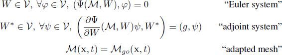
by a discrete one and then solve it. For discretizing the state and adjoint PDEs, we take the spatial schemes introduced previously that are explicit Runge–Kutta time-advancing schemes. Such time discretization methods have nonlinear stability properties like TVD, which are particularly suitable for the integration of system of hyperbolic conservation laws where discontinuities appear. Discretizing the last equation consists of specifying the mesh according to a discrete metric deduced from the discrete states. In Chapter 2 of Volume 1, we describe a TFP that avoids the generation of a new mesh at each solver iteration, which otherwise would imply serious degradation of the CPU time and the solution accuracy due to the large number of mesh modifications. It is also an answer to the lag problem occurring when, from the solution at tn, a new adapted mesh is generated at level tn to compute next solution at level tn+1. The basic idea consists of splitting the simulation time frame [0, T] into nadap adaptation sub-intervals:
and to keep the same adapted mesh for each sub-interval. Consequently, the time-dependent simulation is performed with only nadap different adapted meshes. The mesh used on each sub-interval is adapted to control the solution accuracy from ti−1 to ti. We examine now how to apply this program when a GO approach is chosen.
7.6.1. Choice of the GO metric
The optimal adapted meshes for each sub-interval are generated according to analysis of section 7.4.5. In this work, the following particular choice has been made:
– the Hessian metric for sub-interval i is based on a control of the temporal error in L∞ norm:
– the function τ : t ⟼ τ(t) is constant and equal to 1;
– all sub-intervals have the same time length Δt.
The optimal GO metric ![]() then simplifies to
then simplifies to
REMARK 7.3.– We note that we obtain a similar expression of the optimal metric to the one proposed in Alauzet and Olivier (2011), but it is presently obtained in a GO context and by means of a space–time error minimization.
7.6.2. Global fixed-point mesh adaptation algorithm
To converge the nonlinear mesh adaptation problem, that is, converging the couple mesh solution, we propose a fixed-point mesh adaptation algorithm. The parameter Nst representing the total computational effort is prescribed by the user and will influence the size of all the meshes defined during the time interval. That is, to compute any metric fields ![]() we have to evaluate a global normalization factor that requires the knowledge of all
we have to evaluate a global normalization factor that requires the knowledge of all ![]() Thus, the whole simulation from 0 to T must be performed to be able to evaluate all metrics
Thus, the whole simulation from 0 to T must be performed to be able to evaluate all metrics ![]()
Note that passing to a global – over [0,T] – adaptation iteration is solely an option when a feature-based adaptation is chosen (e.g. Alauzet and Olivier 2011). In contrast, choosing the GTFP mesh adaptation algorithm (Algorithm 7.1) is compulsory for the GO approach.
Algorithm 7.1. Global transient fixed-point mesh adaptation algorithm
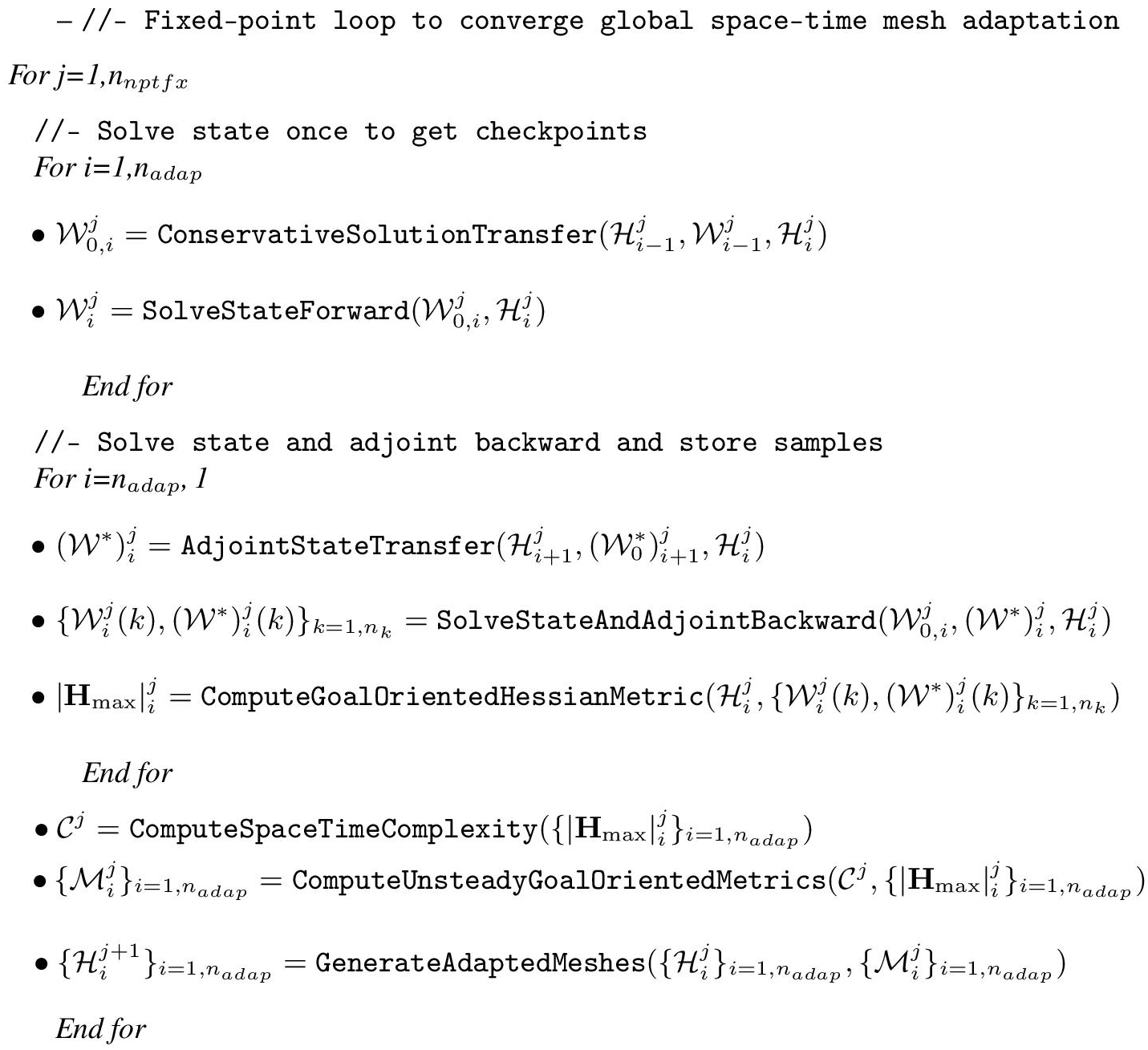
Let us describe this algorithm also sketched in Figure 7.6. It consists of splitting the time interval [0,T] into the nadap mesh-adaptation time sub-intervals: ![]() with t0 = 0 and
with t0 = 0 and ![]() . On each sub-interval, a different mesh is used. A time-forward computation of the state solution is first performed with an out-of-core storage of all checkpoints, which are taken to be
. On each sub-interval, a different mesh is used. A time-forward computation of the state solution is first performed with an out-of-core storage of all checkpoints, which are taken to be ![]() . Between each sub-interval, the solution is interpolated on the new mesh using the conservative interpolation of Alauzet and Mehrenberger (2010). Then, starting from the last sub-interval and proceeding until the first one, we recompute and store in memory all solution states of the sub-interval from the previously stored checkpoint in order to evaluate time-backward the adjoint state throughout the sub-interval. At the same time, we evaluate the Hessian metrics
. Between each sub-interval, the solution is interpolated on the new mesh using the conservative interpolation of Alauzet and Mehrenberger (2010). Then, starting from the last sub-interval and proceeding until the first one, we recompute and store in memory all solution states of the sub-interval from the previously stored checkpoint in order to evaluate time-backward the adjoint state throughout the sub-interval. At the same time, we evaluate the Hessian metrics ![]() required to generate new adapted meshes for each sub-interval. To this end, a number
required to generate new adapted meshes for each sub-interval. To this end, a number
nk of Hessian metric samples are computed on each sub-interval and intersected in the sense of the metric intersection defined in section 3.6.1 to obtain ![]() At the end of the computation, the global space–time mesh complexity is evaluated, producing weights for the GO metric fields for each sub-interval. Finally, all new adapted meshes are generated according to the prescribed metrics. The time-forward, time-backward and mesh update steps are repeated into the j = 1, .., nptfx global fixed point loop. Convergence of the fixed point is obtained in typically five global iterations.
At the end of the computation, the global space–time mesh complexity is evaluated, producing weights for the GO metric fields for each sub-interval. Finally, all new adapted meshes are generated according to the prescribed metrics. The time-forward, time-backward and mesh update steps are repeated into the j = 1, .., nptfx global fixed point loop. Convergence of the fixed point is obtained in typically five global iterations.
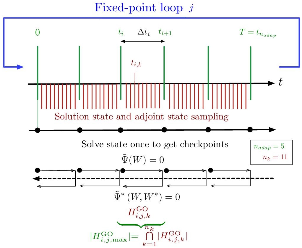
Figure 7.6. Global transient fixed-point algorithm for unsteady goal-oriented anisotropic mesh adaptation. For a color version of this figure, see www.iste.co.uk/dervieux/meshadaptation2
This mesh adaptation loop has been fully parallelized. The solution transfer, the solver and the Hessians computation have been parallelized using a p-thread paradigm at the element loop level (Alauzet and Loseille 2009b). With regard to the computation of the metrics and the generation of the adapted meshes, we observe that they can be achieved in a decoupled manner once the complete simulation has been performed, leading to an easy parallelization of these stages. Indeed, if nadap processors are available, each metric and mesh can be done on one processor.
7.6.3. Computing the GO metric
The optimal GO metric is a function of the adjoint state values, the adjoint state spatial gradients, the state time derivative, Hessian and the Euler fluxes Hessians. In practice, these continuous states are approximated by the discrete states and derivative recovery is applied to get gradients and Hessians. The discrete adjoint state ![]() is taken to represent the adjoint state W∗. The gradient of the adjoint state ∇W∗ is replaced by
is taken to represent the adjoint state W∗. The gradient of the adjoint state ∇W∗ is replaced by ![]() and the Hessian of each component of the flux vector H(Fi(W)) is obtained from HR(Fi(Wh)). ∇R (respectively, HR) stands for the operator that recovers numerically the first (respectively, second) order derivatives of an initial piecewise linear solution field. In this chapter, the recovery method is based on the L2-projection formula, as explained in section 5.4.
and the Hessian of each component of the flux vector H(Fi(W)) is obtained from HR(Fi(Wh)). ∇R (respectively, HR) stands for the operator that recovers numerically the first (respectively, second) order derivatives of an initial piecewise linear solution field. In this chapter, the recovery method is based on the L2-projection formula, as explained in section 5.4.
7.7. Numerical experiments
The adaptation algorithms described in this chapter have implemented the CFD code Wolf. We use Yams (Frey 2001) for the adaptation in 2D and Feflo.a (Loseille and Löhner 2010) in 3D.
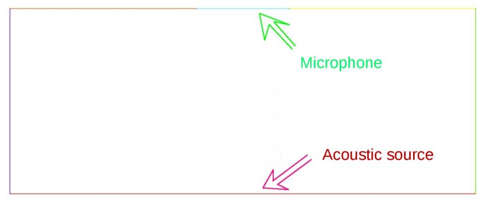
Figure 7.7. Propagation in a box: sketch of geometry. An acoustic source produces sound at the center of the bottom. The microphone integrates the pressure variation on a segment of the top wall. For a color version of this figure, see www.iste.co.uk/dervieux/meshadaptation2
7.7.1. 2D Acoustic wave propagation
A typical example of pressure deviation propagating over long distances is linear acoustics. Linear acoustic waves usually refer either to a transient wave of bounded duration or to a periodic vibration. An important context in the study of these different kinds of waves is when we are interested only in the effect, during a limited time-interval, of the wave on a microphone occupying a very small part of the region affected by the pressure perturbation. Further simplifying, we can be interested in a single scalar measure of this effect, for instance the total energy Etot received by the sensor during a given time interval. If the pressure perturbation is emitted at a very long distance in an open and complex spatial domain, the numerical simulation of this phenomenon can be extremely computer intensive, if not impossible. In Belme et al. (2012), the authors consider an acoustic source s (A =0.01, B = 256, C = 2.5 and f = 2):
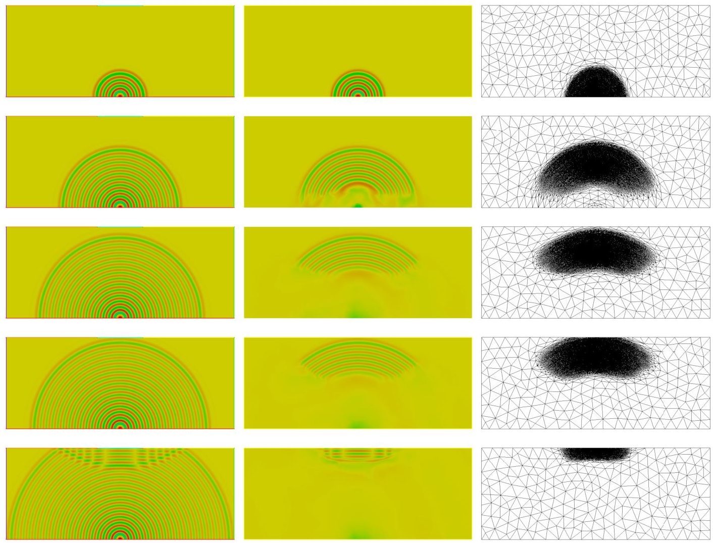
Figure 7.8. Propagation of acoustic waves: density field evolving in time on a uniform mesh (left) and on adapted meshes (middle and right). For a color version of this figure, see www.iste.co.uk/dervieux/meshadaptation2
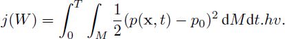
We analyze the sound signal emitted by this source on a microphone M located at the center-top of the domain. The GO mesh adaptation considers the cost function
The time interval of the simulation is split into 40 sub-intervals (thus 40 checkpoints are used) and six fixed-point iterations are applied in order to converge the mesh adaptation problem. As expected, mesh adaptation reduces as much as possible mesh fineness in parts of the computational domain where accuracy loss does not influence the quality of sound prediction on the microphone. This is illustrated in Figure 7.8. The numerical convergence order is a central measure for evaluating the quality of adaptation. The scalar which we observe is the integrand k(t) of the functional on the micro M, k(t) = ∫ (p − p0)dM . More precisely, we measure the amplitude of the first wave attainingMM. With a sequence of uniform meshes with 60,000, 80,000 and 117,000 vertices, we obtain a poor convergence order of 0.6, while with a sequence of adapted meshes with 1,200, 24,000 and 64,000 vertices in the average, the spatial convergence order is 1.98.
7.7.2. 3D blast wave propagation
Finally, the last example, also taken from Belme et al. (2012), considers a three-dimensional blast wave propagation in a complex geometry representing a city square surrounded by buildings. On the floor of the square we have a small half-sphere with high pressure and high density while the rest of atmosphere is standard. Cost function j is again the quadratic deviation from ambient pressure on target surface Γ, which is composed of one particular building (Figure 7.9):
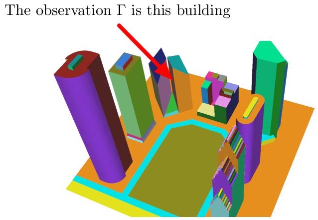
Figure 7.9. 3D City test case geometry and location of target surface Γ (surface of the building indicated by the arrow). For a color version of this figure, see www.iste.co.uk/dervieux/meshadaptation2
The simulation time frame is split into 40 time sub-intervals, that is, 40 different adapted meshes are used to perform the simulation. Six fixed-point iterations are performed to converge the mesh adaptation problem. For each sub-interval, 16 samples of the solution and adjoint states are considered to build the GO metric. The space–time complexity is prescribed at 1.2 million.
The resulting adjoint-based anisotropic adapted meshes (surface and volume) for both simulations at sub-interval 10, 15 and 20 are shown in Figure 7.10. Despite the complexity and the unpredictable behavior of the physical phenomena with a large number of shock waves interactions with the geometry, the GO fixed point mesh adaptation algorithm is automatically able to capture those shock waves, which impact the targeted buildings and to set appropriate weights for the refinement of these physical phenomena. Other waves are neglected thus leading to a drastic reduction of the mesh size. To illustrate this point, we provide meshe sizes for sub-intervals 1, 5, 10 and 20 in Table 7.1, where nv, nt and nf are the number of vertices, tetrahedra and triangles, respectively, and h the mesh size. If, for sub-interval 1, 1 million vertices is needed, only 40,000 vertices are used for sub-interval 20. On average, almost 200,000 vertices are required with a maximal accuracy between 1 and 5 cm. These numbers have to be compared with 33,000,000, the number of vertices for an uniform mesh with accuracy of the order of cm. With regard to the amount of anisotropy achieved for these simulations, mesh anisotropy can be quantified by two different indicators: the anisotropic ratios and quotients, according to definition 3.19. The anisotropic ratio stands for the maximum elongation of a tetrahedron by comparing two principal directions. For both simulations, an average anisotropic ratio between 7 and 16 is achieved. The anisotropic quotient represents the overall anisotropic ratio of a tetrahedron taking into account all the possible directions, we get a mean anisotropic quotient between 40 and 200. This quotient can be considered as a measure of the overall gain in three dimensions of an anisotropic adapted mesh as compared to an isotropic adapted one.
Table 7.1. Mesh characteristics of the 3D blast wave calculation. For anisotropic ratio and quotient of an element, see definition 3.19 in Volume 1
| Iteration | nv | nt | nf | min h | Ratio avg. (max) | Quotient avg. (max) |
|---|---|---|---|---|---|---|
| 1 | 1,058,084 | 6,177,061 | 79,862 | 1. cm | 9 (62) | 63 (2,242) |
| 10 | 249,620 | 1,427,956 | 34,318 | 1.2 cm | 16 (94) | 197 (5,136) |
| 15 | 72,432 | 392,970 | 24,678 | 2.1 cm | 12 (76) | 119 (3,789) |
| 20 | 40,297 | 205,855 | 21,980 | 4.8 cm | 7 (64) | 39 (3,547) |
| Avg. | 188,357 | 1,074,777 | 28,811 |
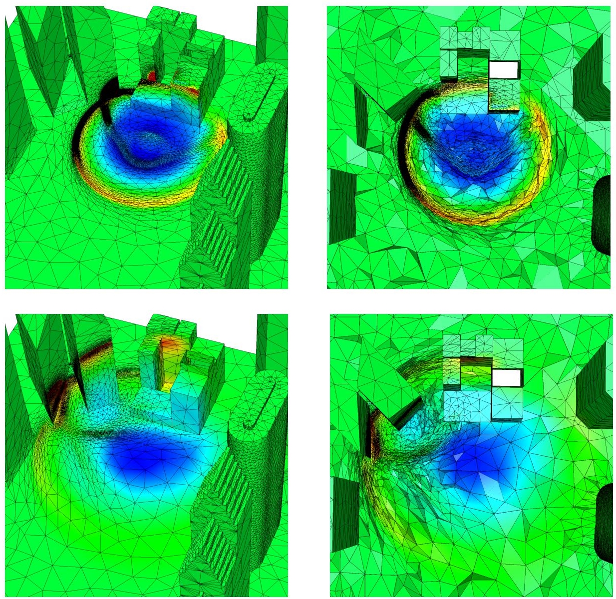
Figure 7.10. 3D Blast wave propagation: adjoint-based adapted surface (left) and volume (right) meshes at sub-intervals 10 and 20 and corresponding solution density at a-dimensioned times 5 and 10. For a color version of this figure, see www.iste.co.uk/ dervieux/meshadaptation2
7.8. Conclusion
This chapter introduces the GTFP mesh adaptation algorithm, which involves the specification of the set of spatial meshes used in an unsteady simulation as the optimum of a GO error analysis. This method specifies both mesh density and mesh anisotropy by variational calculus. Accounting for unsteadiness is applied in a time-implicit mesh-solution coupling, which needs a nonlinear iteration, the fixed point. In contrast to the Hessian-based fixed-point mentioned in Chapter 2 of this volume that iterates on each sub-interval, the new GTFP covers the whole time interval, including forward steps for evaluating the state and backward ones for the adjoint. This algorithm successfully applies to 2D and 3D blast wave Euler test cases and to the calculation of a 2D acoustic wave. Results demonstrate the favorable behavior expected from an adjoint-based method, which gives an automatic selection of the mesh regions necessary for the target output.
Several important issues for fully space–time computation have been addressed. Among them, the strategies for choosing the splitting in time sub-intervals and the accurate integration of time errors in the mesh adaptation process have been proposed, together with a more general formulation of the mesh optimization problem.
Time discretization error is not considered in this study. Solving this question is not so important for the type of calculations that are shown in this chapter, but can be of paramount impact in many other cases, in particular when implicit time advancing is considered.
7.9. Notes
More computational examples are given in Belme et al. (2012).
Link with further work. As mentioned in Chapter 4 of this volume, the proposed error analysis relies on the interpolation errors committed on the 15 Euler fluxes. In Chapter 5 of this volume, we introduce a linearized version in which it is enough to consider the interpolation errors on conserved unknowns. Although the linearized version has been tested only on steady viscous flow, it is probable that its accuracy in the unsteady viscous context can be better than the accuracy of the analysis presented in this chapter.