
2
Multi-scale Adaptation for Unsteady Flows
In this chapter, we describe an extension of the multiscale feature-based mesh adaptation method for the calculation of an unsteady flow. The mesh adaptation relies on a metric-based method controlling the Lp-norm of the spatial interpolation error. Mesh-adaptive time advancing is achieved because of a transient fixed-point adaptation algorithm to predict the solution evolution coupled with a metric intersection in time procedure. In time direction, we impose equidistribution of error, that is, minimization in L∞. This adaptive approach is illustrated with an incompressible two-phase flow using a level set formulation.
2.1. Introduction
Multi-scale metric-based mesh adaptation methods need to be carefully extended before they efficiently apply to unsteady flows. We restrict our discussion to numerical unsteady schemes using time advancing. We consider adaptation methods changing the spatial mesh during the simulation time frame. Two options are usually considered. In the first option, mesh changes during the time advancing, for instance, between tn and tn+1. Due to the difficulties in building a time derivative between meshes of different connectivities, the mesh is generally only deformed, for example, as in the moving finite element (Baines 1994). In the second option, the mesh does not change during the time advancing, but instead at a time level, for example, tn. Once the mesh is changed, the solution is advanced from tn to tn+1 with the new mesh. It may happen that a good mesh for level tn is a bad one for tn+1.For example, this happens when a shock is moving. For a robust accuracy, the mesh need to be adapted not only for level tn but also for level tn+1. In many papers, a device is found in order to anticipate the evolution during the corresponding time interval [tn,tn+1]. In contrast, in the present chapter, the adequation of the mesh with the concerned time levels is obtained by a fixed point algorithm, which generalizes to time advancing the Hessian-based steady-state fixed point described by Algorithm 5.1. in Chapter 5 of Volume 1. This extension is the transient fixed-point (TFP) mesh adaptation algorithm initiated in Alauzet et al. (2007). In this algorithm, the solution evolution through a specified time interval, involving one or several solver time steps, is first predicted, then the mesh is adapted to the predicted solution evolution because of the metric intersection between the time levels involved in the considered time interval. Finally, the solution is advanced with the new adapted mesh.
In this chapter, the TFP is introduced and analyzed in order to approach the early capturing (EC) property for spatial error and, at least, to show a predictable mesh convergence rate that will be better than with non-adaptive approaches. To demonstrate the efficiency of the proposed approach, we concentrate on an unsteady flow model involving discontinuities, namely the incompressible two-phase model defined and discretized in Chapter 1 of Volume 1. Calculations involve the advection of a discontinuous density and deals with discontinuities (density, viscosity) in momentum equations. If in such a calculation the interface is not fitted by the mesh (like, for example, in a Lagrangian mode), then its numerical capturing may induce a deterioration of convergence order. The level set method is a mean for increasing the smoothness of the interface advection problem. An analysis in Chapter 1 of Volume 1 predicts an order of 4/3 for Euler flows, but this analysis does not extend to Navier–Stokes flows. In the velocity/momentum equations, the flow variables have discontinuous properties (density, viscosity) near the interface and accuracy order is limited to one. These discontinuities could be addressed with a sophisticated discontinuous approximation like the ghost fluid method (GFM) (Fedkiw et al. 1999), with the hope that most part of the singularities are taken into account in order to recover a high-order accuracy. We do not consider GFM in this chapter; instead, a thickened interface method is applied. These discontinuous properties are smoothed by replacing the discontinuity by a sinusoidal transition. But if no mesh adaptation is used, this may limit the accuracy to first order.
In this chapter, we keep the basic option of a feature-based adaptation, that is, we make the assumption that the discretization error can be controlled by the interpolation error of some features prescribed by the user, as done in the previous chapters. We combine several error criteria for adapting the mesh: first, to the momentum equations, and second, to the level set advection. We describe a method for controlling, time interval after time interval, the error of transient flows. It relies on the maximum in time of the instantaneous Lp norm of spatial error. We explain how to introduce this strategy in the transient fixed point mesh adaptation algorithm. Conditions for faster convergence to the continuous solution are discussed. This method is applied to several simplified and more complex test cases in order to evaluate the resulting gain in accuracy and convergence. Sections 2.2 and 2.3 present the central issues of mesh adaptation with notably the transient fixed point mesh adaptation algorithm and the specific adaptation to the interface. Then, in section 2.4, the impact of the proposed algorithm on the solution accuracy and the numerical convergence is analyzed on a two-dimensional example. Finally, in section 2.5, this approach is validated on a realistic three-dimensional example for which experimental data are available.
2.2. Mesh adaptation efficiency
Two new difficulties are addressed in this chapter. First, we consider an unsteady flow. Our numerical model is a time-advancing model and we have to consider how frequently the spatial mesh needs to be changed. Second, we consider a flow with a discontinuous (moving) interface, which will need to be captured accurately by the adapted mesh.
2.2.1. Regular and singular unsteady model
As explained in section 2.9 of Volume 1, several new issues must be considered for mesh adaptation in the unsteady case.
2.2.1.1. Space-time convergence analysis for unsteady calculations
The numerical approximation order can be evaluated on the basis of a space–time convergence, over the cylinder Q = Ω × [0, T]. For this, the extended definition of convergence order ![]() still applies. For a 3D unsteady simulation, the dimension d is set to 4; the total number of degrees of freedom N representing the approximate space–time function is the total number, time level after time level, of the spatial nodes used during the unsteady calculation. In the case of uniform meshes with m nodes and n time levels, N = m × n. Another equivalent way to express a convergence order at least equal to α is to compare two embedded discretizations, namely for N and kd N degrees of freedom:
still applies. For a 3D unsteady simulation, the dimension d is set to 4; the total number of degrees of freedom N representing the approximate space–time function is the total number, time level after time level, of the spatial nodes used during the unsteady calculation. In the case of uniform meshes with m nodes and n time levels, N = m × n. Another equivalent way to express a convergence order at least equal to α is to compare two embedded discretizations, namely for N and kd N degrees of freedom:
Let us focus, for example, on the motion of a step function in a fixed 3D spatial domain uniformly meshed. We assume that the space–time approximation is second-order far from the discontinuity and first-order (in L1) at the discontinuity vicinity. Due to the first-order accuracy (α = 1) around the discontinuity, it is mandatory that both spatial step and time step to be four times smaller (k = 4) to get a four times smaller error. In other words, starting from a solution uN obtained with a total of N degrees of freedom, the approximation error will be four times smaller only with a total number of degrees of freedom of 4d N = 256N:
On the contrary, we could want to recover the maximal convergence order of the numerical scheme, here order two, on this discontinuous solution, that is, to use only 24 N = 16N for an error again four times smaller. To obtain this, it is necessary to concentrate the mesh adaptively near the discontinuity with a space–time mesh. The space–time meshing option is generally not considered in the literature because it needs, among many disadvantages, to mesh in 4D and to reformulate the numerical scheme. In contrast to space–time meshing, we restrict ourselves to time-advancing schemes, which means that the space–time mesh is constrained to be built from constant–time plans. For the same accuracy, the number of degrees of freedom of time-advancing approximations maybe larger than for space–time meshing. To reduce the time error by a factor of four in our example, the number of time levels needs to be four times larger. This factor four will multiply the spatial mesh refinement ratio.
A barrier limiting the convergence order in the presence of singularities at a maximum of 8/5 written as
has been identified in lemma 2.9 in Volume 1.
2.2.2. Representativity of the spatial interpolation error
We assume now that satisfying the usual explicit stability condition implies that the time error is of the same size as the space error. We discuss the validity of this assumption in section 2.7. With the above assumption, we are equipped with an error field at each time level, which then discretizes a space–time error field. Let us discuss which space–time norm we want to minimize. Let us compare between minimizing the error in the norm in ![]()
The first option Lq(0, T; Lp(Ω)) would be coherent with the steady-state multiscale Lp theory of Chapter 5 of Volume 1, but taking it would imply that the space– time mesh can be updated only after the computation of the whole simulation time frame, in order to control the global space–time complexity or the global space–time error in Lq(0,T; Lp(Ω)). Such a global approach is discussed in Chapter 7 of this volume.
As concerns the second option of L∞(0, T; Lp(Ω)), we have seen in Chapter 4 of Volume 1 that L∞-based adaptation does not produce second-order convergence. But since we are applying spatial adaptation, the L∞(0, T; Lp(Ω)) approach will be able to spatially capture discontinuities and the error Lp norm of spatial approximation at each time level can be driven to small values. The L∞ in time strategy consists of requirement that each mesh fulfills a specified Lp-error=ε criterion. Adaptative spatial order is maintained at level 2 as in the first option, while, as for the first option, time accuracy constraint leads to divide the timestep by 4, as for the first option, so that the 8/5 limit can also be attained. We then feel free to select the L∞(0, T; Lp(Ω)) space–time adaptation criterion, which we could apply as in Algorithm 2.1.
Algorithm 2.1. Transient fixed-point mesh adaptation with a new mesh every time step
Now, Algorithm 2.1 is not satisfying. Indeed, an algorithm changing the mesh at each solver time step in order to adapt it to the solution evolution has two bottlenecks. First, it increases drastically the cost in terms of mesh generation. Second, it introduces a large amount of error due to the transfers of the solution field from one mesh to another as the new adapted mesh is not a simple deformation of the first one. These issues are motivations to use a spatial mesh during several time steps.
2.3. Transient fixed-point mesh adaptation scheme
The simulation time frame [0, T] is split into several subintervals:
The whole algorithm is presented in Algorithm 2.2. and depicted in Figure 2.1.
The external loop goes from the first subinterval to the last one. On any subinterval [ti, ti+1] is applied a fixed-point iteration, combining alternatively solution computation and mesh regeneration, which corresponds to the internal loop shown in Figure 2.1.
In the internal loop, knowing the spatial mesh, the time subinterval [ti,ti+1] is divided into m time-integration intervals ![]() , with k = 0, ..., m and
, with k = 0, ..., m and ![]() , .
, . ![]() For
For ![]() the solution is given by interpolation from a previous mesh, and for any k = 0, ..., m − 1, the flow variables are advanced from time level
the solution is given by interpolation from a previous mesh, and for any k = 0, ..., m − 1, the flow variables are advanced from time level ![]() to time level
to time level ![]() by means of the numerical scheme. Then, a single metric for the whole subinterval [ti, ti+1] can be defined by intersecting for all k = 0, ..., m the metrics associated with solutions at time level
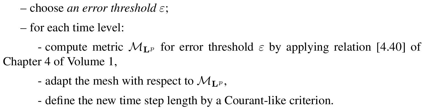
by means of the numerical scheme. Then, a single metric for the whole subinterval [ti, ti+1] can be defined by intersecting for all k = 0, ..., m the metrics associated with solutions at time level ![]() . In practice, not all metrics are intersected, but a few tens of them. The metric intersection procedure is explained in section 3.6 of Volume 1. Then, a new adapted mesh is generated according to this metric and to the error threshold ε. Then either the computation starts again from the same interpolation of the solution obtained at the end of previous subinterval, or this internal loop is stopped, according to a measure of the iterative convergence, namely when the deviation between two successive solutions at ti+1 is sufficiently small, as for the steady case.
. In practice, not all metrics are intersected, but a few tens of them. The metric intersection procedure is explained in section 3.6 of Volume 1. Then, a new adapted mesh is generated according to this metric and to the error threshold ε. Then either the computation starts again from the same interpolation of the solution obtained at the end of previous subinterval, or this internal loop is stopped, according to a measure of the iterative convergence, namely when the deviation between two successive solutions at ti+1 is sufficiently small, as for the steady case.
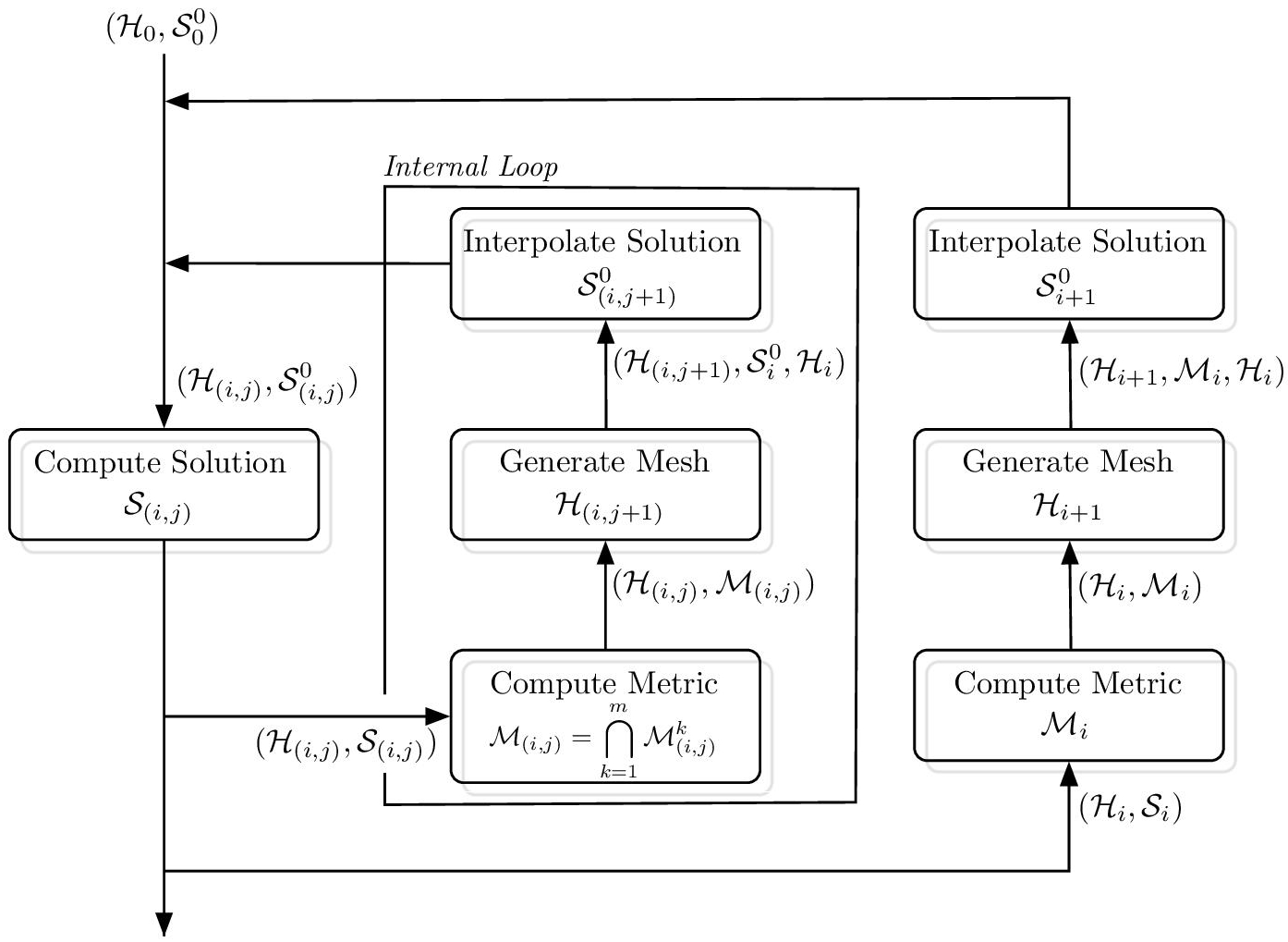
Figure 2.1. Schematic presentation of the transient fixed-point mesh adaptation algorithm. Symbols H, S and M stand for, respectively, mesh, flow solution and metric. The internal loop applies the fixed point process that ensures after its convergence that the spatial mesh used for advancing from ti to ti+1 is adapted to any intermediate flow. The external loop organizes the transition from the end of interval [ti, ti+1] to the beginning of [ti+1, ti+2]
The next action is performed by the external loop that starts the next internal fixed point adaptation loop for [ti+1, ti+2].
Algorithm 2.2. Transient L∞(0, T; Lp (Ω)) fixed-point mesh adaptation algorithm
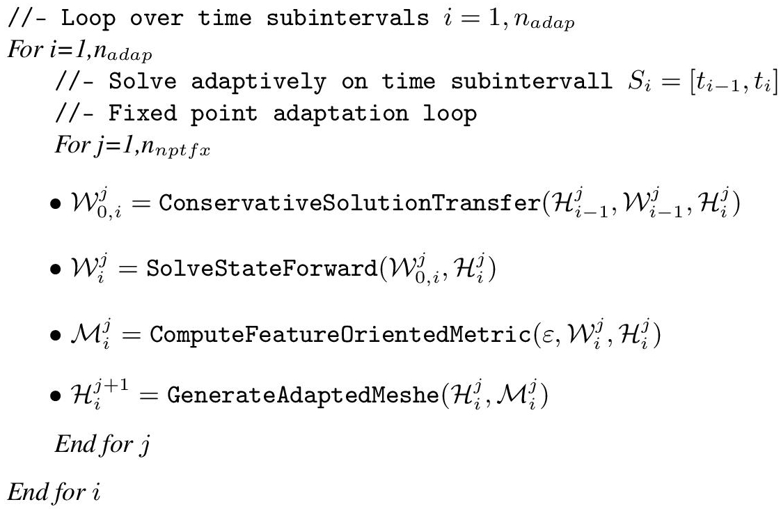
For each subinterval, a maximal metric ![]() is computed from the different variables and different time levels of the subinterval by applying the metric intersection defined in section 3.6.1.
is computed from the different variables and different time levels of the subinterval by applying the metric intersection defined in section 3.6.1.
The number nadap of adaptation time intervals [ti, ti+1] is an extra discretisation parameter to be specified. Let us again consider the case of a discontinuity traveling across the spatial domain, from one side to the opposite one.
If we compute with a unique anisotropic adaptation time interval (nadap = 1), that is, [t0, t1] = [0,T], the final unsteady calculation is performed on one mesh, adapted to all intermediate positions of the discontinuity, which, in this particular example, results in a uniform fine mesh. In that case, the mesh adaptation cycles do not result in a better efficiency. Instead, convergence remains at first order or less.
Conversely, if the number nadap of adaptation time intervals [ti, ti+1] is too large, this results in (1) the costly generation of a very large number of meshes and (2) too many transfers between adapted meshes resulting in the accumulation of a large error. Therefore, for a single mesh adaptive calculation, a compromise needs to be found between the above limiting options. In the numerical example, we shall define a compromise that can be used.
2.3.1. Size of subintervals in a mesh convergence
A second question is: how these adaptation time intervals should be chosen in a strategy of several calculations for mesh convergence to continuous solution. To illustrate the impact of the time-interval size on the adapted mesh, we consider the advection by a constant velocity a discontinuity. Figure 2.2 shows the adapted mesh for the time period [ti, ti+1] (on both pictures), the mesh use for the travel of a circle-shaped discontinuity. When advected, the circular discontinuity travels only in the refined regions.
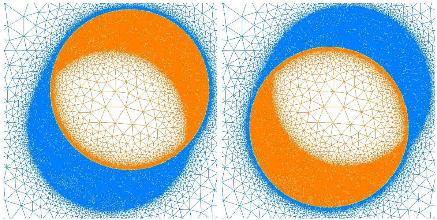
Figure 2.2. Transient fixed-point mesh adaptation algorithm applied to the advection of a circle-shaped discontinuity between a region where physical density is equal to 1 (blue) a region where it is equal to 2 (orange). Left, the interface at time ti. Right, the interface at time ti+1. On both pictures, the adapted mesh for advection during the time interval [ti, ti+1]. For a color version of this figure, see www.iste.co.uk/dervieux/meshadaptation2
Let us assume that we keep the same subinterval [ti, ti+1] for the different computations of a mesh convergence. In order to reduce the error by a factor of four in 3D, we wish to divide the error by a factor of four by performing two successive computations:
– one with a coarse Mesh 1 with a mesh size of N nodes;
– one with a fine Mesh 2 with a mesh size of 8N nodes.
The finely discretized vicinity of the discontinuity, which is defined by the trajectory of it during the time interval, will cover the same region of the computational domain as for the coarse computation. Then, if the isotropic mode is chosen, the number of nodes inside this “vicinity of discontinuity” will pass from Nd for Mesh 1 to 64Nd for Mesh 2 since the local Δx is divided by 4. This should be 8Nd for second-order convergence. In this example, second-order spatial convergence is clearly unreachable. The region of high refinement swept by the discontinuity needs to be reduced by a factor of eight, which shows that the adaptation time intervals [ti, ti+1] should be taken eight times smaller for the calculation with Mesh 2. In the anisotropic mode, the situation is much better, since running for Mesh 2 with the same adaptation time intervals as Mesh 1 would result in passing from Nd for Mesh 1 to a Mesh 2 in which, in a favorable case, only the mesh size normal to discontinuity needs to be four times smaller, while the two other directions are two times smaller, which results in a number of 16Nd (still larger than 8Nd, second order). However, if in these conditions the time intervals are divided by two, then we get a number of 8Nd:
LEMMA 2.1.– In the 3D anisotropic case, a necessary condition for second-order spatial convergence is that subintervals [ti, ti+1] are two times smaller for a four times smaller spatial error. □
In the sequel, mesh convergence experiments will follow this rule except when mentioned.
2.3.2. Mesh adaptation for unsteady Euler/Navier–Stokes equations with thickened interface
2.3.2.1. Control of interface thickening
For simplicity, we assume in this section that the mesh is adapted at each time step. We discuss how the mesh efforts need to be balanced between the interface capture and the rest of flow resolution. Our numerical model, presented in section 1.3 of Volume 1 relies on a thickened interface. The sine transition with thickness η is introduced in section 1.3.3.2 of Volume 1 for spatial stability purpose. This transition does not need to be computed with a high accuracy. But the thickness η itself introduces an error with respect to the non-discretized solution, which has an interface with zero thickness. The error introduced by interface thickening is a O(η) term. Therefore, the parameter η should tend to zero at convenient rate when the number of vertices N is increased or, equivalently, when the error parameter ε is decreased for convergence toward the continuous solution. For a convergence order α, η should satisfy:
Here, we are interested in being close to second-order convergence. To this end, dividing the global approximation error by a factor of four requires that we multiply the mesh size by two or, equivalently, the mesh density by a factor of 2d in smooth regions of the domain, while we need to divide the thickness η by at least a factor of four. Therefore, choosing the interface thickening η proportional to the specified error level ε provides an equilibrated error behavior in the sense that dividing ε by a factor of four gives a global error divided by four. In practice, we start with a quasi uniform mesh and we set η to a size of 2-3 space steps Δx. In the case of a fixed interface, the convergence is analyzed as follows:
LEMMA 2.2.– Let us assume that the interface does not move during the time interval. Then, the proposed approach with η(ε) = Cst ε has a second-order spatial convergence rate for anisotropic adaptation while the order is at most d/(d − 1) for the isotropic one1. □
While the thickness coefficient η controls the interface thickness, the thickness of mesh refinement near interface is much larger, due to the freezing of mesh on each time subinterval. We assume that the extra thickness due to η can be neglected. Then lemma 2.1 can still be applied.
2.3.2.2. Local criterion for bi-fluid flows
We now discuss a heuristic choice of criterion designed to accurately capture the interface when a level set method is applied. In the context of bi-fluid flows, it is important to specify which quantities – the features – are going to govern the mesh adaptation according to the error analysis introduced in Chapter 5 of Volume 1.
First, the mesh is adapted to compute accurately the dynamic of the flow. Indeed, capturing small-scale details can be determinant for the final overall accuracy. To this end, the momentum length ρ|U| is used as an adaptive variable and its interpolation error is controlled in L2 norm. This provides ![]()
Second, the mesh has to be adapted to the thickened interface to control the error in capturing it. Moreover, it is important to accurately represent the interface curvature for solution accuracy. Two strategies have been considered. As the interface represents a jump of the density, or a sine variation of the density in the case of a thickened interface, a first approach is to adapt, according to Chapter 5 of Volume 1, the mesh to the density: ![]() Although it performs well, this approach has the following weaknesses:
Although it performs well, this approach has the following weaknesses:
– for thickened interfaces, the density Hessian is zero in the middle of the sine variation leading to a coarser mesh in this area;
– it does not take into account the curvature of the interface;
– this adaptation is highly dependent on the specified thickness η.
We thus propose a second strategy where a metric is specifically dedicated to the interface. It is based on a metric that follows the iso-lines of the given field.
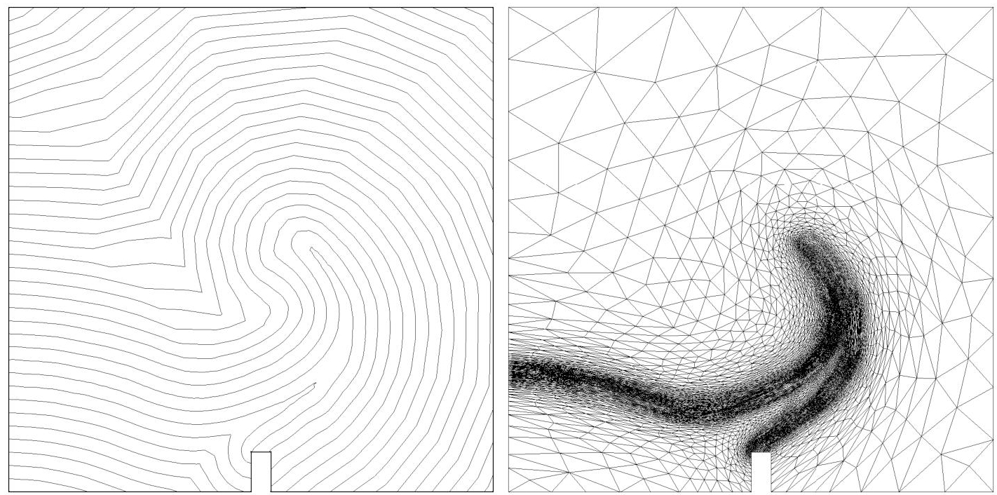
Figure 2.3. Adaptation to the interface, that is, to the 0 value of a level set function ϕ, with the metric given by relation [2.4]. Left, the level set (iso-lines) representation of the function ϕ. Right, the mesh adapted only to the interface
The metric ![]() is dedicated to the interface, that is, only to the 0 contour of the level set function ϕ, which is derived from the iso-lines metric
is dedicated to the interface, that is, only to the 0 contour of the level set function ϕ, which is derived from the iso-lines metric ![]() . This metric for the interface is defined by four parameters:
. This metric for the interface is defined by four parameters:
– hls the prescribed size for the direction n normal to the interface;
– δls the thickness of the adapted region on both sides of the interface;
– εls the error threshold for the variation of the interface that controls the size prescription in the tangential direction t;
– hgrad the growth parameter of the mesh while gradually moving further from the interface.
It is given by
with the notation

and with
The reader can refer to Alauzet (2009) for details on the derivation of hn(x) and ht(x). Figure 2.3 displays the adaptation to the interface on the previous example of a breaking water column impacting an obstacle. The level set function ϕ is shown on the left and the adapted mesh generated from the interface metric [2.4] on the right.
To sum up, in the context of bi-fluid flows, a metric for the dynamic of the flow and a metric designed for the interface are computed. Both metrics are taken into account because of the metric intersection defined in section 3.6.1 of Volume 1:
2.3.3. Convergent transient fixed-point
The convergent transient fixed-point also controls mesh refinement in order to converge to the exact solution. This is done through a gain factor R > 1 prescribed by the user. Before re-iteration of the outer loop, according to the choice between complexity controlling or error controlling, either
– the mesh complexity Nm (≈ number of vertices) is increased to Nm+1 = RdNm > Nm, that is, the mesh size is divided by a factor R = (Nm+1/Nm)1/d > 1, or
– the error ε is divided by a factor R2.
In practical cases, we choose R = 21/d (doubling the complexity). We have summarized the above options in Algorithm 2.3.
2.4. 2D bi-fluid example
We present now a convergence study of the 2D version of the proposed adaptive algorithm applied to the complete bi-fluid numerical model presented in section 1.3 of Volume 1 (Niceflow platform) in the context of a bi-fluid flow simulation.
A rectangular water column is falling inside a rectangular box. Measurements have been done by Koshizuka et al. (1995). We compare the convergence of the simulation on structured uniform meshes and adaptive meshes on four outputs that are the position of the interface front at bottom of the box at different times. The first strategy uses a series of embedded structured uniform meshes of sizes between 2,500 and 40,000 vertices. The second strategy uses two outer iterations of Algorithm 2.3. with isotropic meshes and involves two adaptive simulations with error threshold 2 ε and ![]() . The simulation time frame is split into 40 subintervals of 0.025 s for mesh adaptation. As the number of vertices varies for the adaptive simulations, the mean number of vertices of the whole simulation, respectively, 1,800 and 2,700 vertices, is considered for the spatial convergence study. The numerical values of the four outputs of this study are summarized in Table 2.1. The performance in convergence of the calculations is sketched in Figure 2.5. Rather surprisingly, an approximatively second-order numerical convergence is observed for the three uniform mesh computations. This allows to apply a Richardson-type second-order extrapolation to the two finest calculations, giving a probably very accurate estimate of the continuous solution. On the basis of this accurate estimate, we observe that (1) adaptive computations show a higher order spatial convergence (the convergence order is observed with the thickened interfaces), at least on this time interval, and (2) the adaptive computation with an average of 2,700 vertices on one part and the uniform mesh with 40,000 on the other part produce results of same quality.
. The simulation time frame is split into 40 subintervals of 0.025 s for mesh adaptation. As the number of vertices varies for the adaptive simulations, the mean number of vertices of the whole simulation, respectively, 1,800 and 2,700 vertices, is considered for the spatial convergence study. The numerical values of the four outputs of this study are summarized in Table 2.1. The performance in convergence of the calculations is sketched in Figure 2.5. Rather surprisingly, an approximatively second-order numerical convergence is observed for the three uniform mesh computations. This allows to apply a Richardson-type second-order extrapolation to the two finest calculations, giving a probably very accurate estimate of the continuous solution. On the basis of this accurate estimate, we observe that (1) adaptive computations show a higher order spatial convergence (the convergence order is observed with the thickened interfaces), at least on this time interval, and (2) the adaptive computation with an average of 2,700 vertices on one part and the uniform mesh with 40,000 on the other part produce results of same quality.
Algorithm 2.3. Convergent transient fixed-point mesh adaptation algorithm for flow with interface
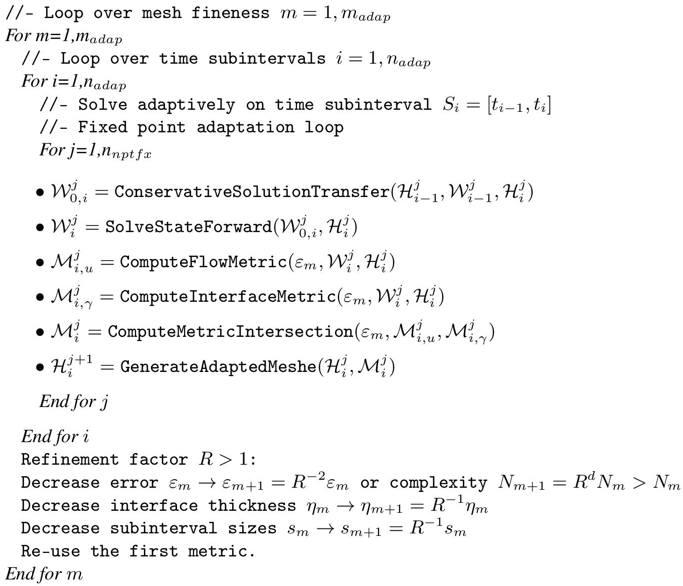
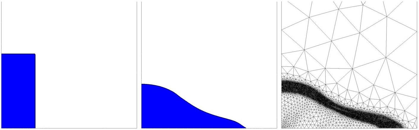
Figure 2.4. 2D falling water column. Interfaces at t = 0 and t = 2 and mesh at t = 2. For a color version of this figure, see www.iste.co.uk/dervieux/meshadaptation2
Table 2.1. 2D falling water column.The x-location of the bottom of the column at different dimensionless time![]() . Spatial convergence is evaluated with three embedded structured uniform meshes (lines 1-3), an extrapolation from these (line 4) and two adaptive mesh simulations (lines 5-6)
. Spatial convergence is evaluated with three embedded structured uniform meshes (lines 1-3), an extrapolation from these (line 4) and two adaptive mesh simulations (lines 5-6)
| Mesh Dimensionless time | 0.5 | 1 | 1.5 | delta/order |
| S1 Structured (2,500 vertices) | 0.732 | 0.939 | 1.374 | 0.093 |
| S2 Structured (10,000 vertices) | 0.736 | 0.982 | 1.442 | 0.025 |
| S3 Structured (40,000 vertices) | 0.740 | 1.013 | 1.461 | 0.006/2.0 |
| S2-S3 Second-order extrapolation | 0.7413 | 1.022 | 1.467 | 0. |
| Adaptive (mean size ≈ 1,800 vertices) | 0.735 | 0.994 | 1.45 | 0.017 |
| Adaptive (mean size ≈ 2,700 vertices) | 0.741 | 1.019 | 1.46 | 0.007/2.1 |
2.5. Example: impact of a 3D water column on a obstacle
This three-dimensional example is presented in detail in Guégan et al. (2010). It aims at validating the proposed method in a long-time simulation involving a 3D complex interface. We use isotropic meshes2. The problem consists of a water column falling in a parallelepipedic box containing a cubic obstacle. This experiment has been performed by the Maritime Research Institute Netherlands (MARIN)3. Water height and pressure measurements are available on a series of points as functions of time. Their positions in the computational domain are shown in Figure 2.6. All test case and experiment data are available on the Smoothed Particle Hydrodynamics European Research Interest Community4 (SPHERIC). The experiment involves a violent transient flow with a very complex interface when the water impacts the obstacle and the opposite wall (at a physical time close to 2 s). Then, the flow returns to a smooth sloshing mode. Several calculations of this case have been presented in the literature (see, for instance, Elias and Coutinho (2007) and Kleefsman et al. (2005)). They illustrate that long-term accuracy is a difficult challenge. The simulation described here5 has been run during a physical time of 6 s, which corresponds to a forward wave motion, a backward one, and then a second forward motion. The mesh adaptation is chosen to be isotropic and follows Algorithm 2.2. The simulation time interval has been split into 120 subintervals of 0.05 s. The interface evolution obtained in this simulation is depicted in Figures 2.7 and 2.8 at different physical times. It is compared to pictures of the MARIN experiment6 (on the right).
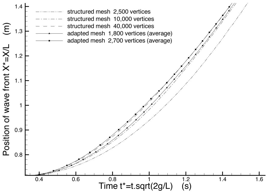
Figure 2.5. 2D falling water column. The x-location of the bottom of the column is presented as a function of time during the early acceleration of the process. Three embedded structured uniform mesh computations and two adaptive mesh computations are compared. See Table 2.1 and text for analysis
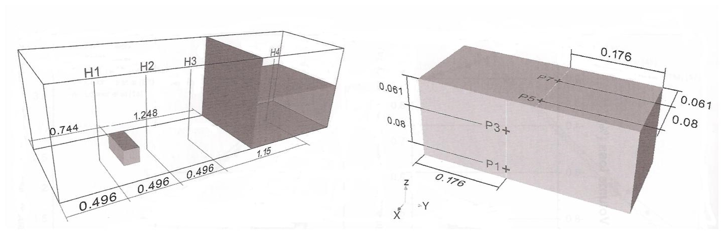
Figure 2.6. 3D falling water column on a obstacle. Left, the simulation geometry with the initial conditions and the position of the water height sensors. Right, the position of the pressure sensors on the obstacle. Pictures courtesy of R.N. Elias and A.L.G.A. Coutinho extracted from Elias and Coutinho (2007)
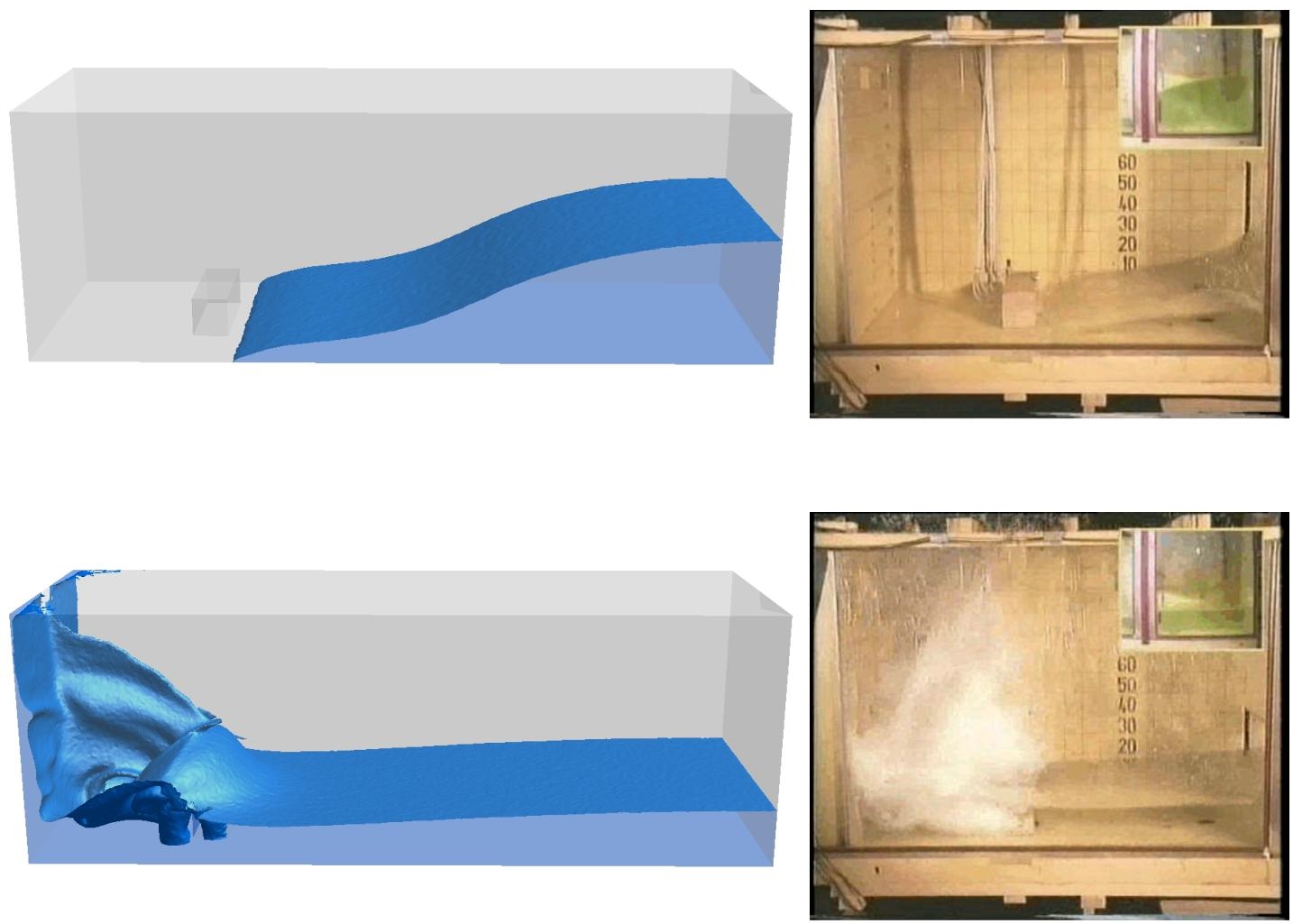
Figure 2.7. 3D falling water column on a obstacle. Comparison between the interface obtained in the simulation (left) and the pictures from the MARIN experiment (right). From top to bottom, snapshots for every 0.4 s, for times t = 0.4 s and t = 1.6 s. For a color version of this figure, see www.iste.co.uk/dervieux/meshadaptation2
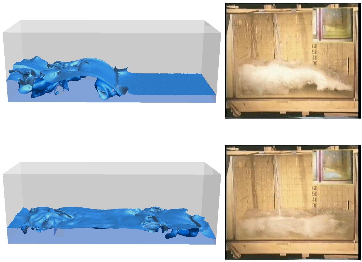
Figure 2.8. 3D falling water column on a obstacle. Comparison between the interface obtained in the simulation (left) and the pictures from the MARIN experiment (right). From top to bottom, snapshots for t = 2.4 s and t = 5.6 s. For a color version of this figure, see www.iste.co.uk/dervieux/meshadaptation2
The interface geometry at physical times 1.6 s and 2.4 s demonstrates the complexity of the simulation, notably by the presence of several tube- and veil-shaped structures for the interface. With a capillarity model, these structures would transform into drops, closer to the physics. The bottom picture of Figure 2.8 shows the return to equilibrium of the flow at time 5.6 s.
An example of the meshes used to advance the solution is presented in Figure 2.9 (left). Figure 2.9 (right) plots the evolution of the number of vertices with respect to the physical time. A detailed comparison with experimental measures is presented in Guégan et al. (2010).
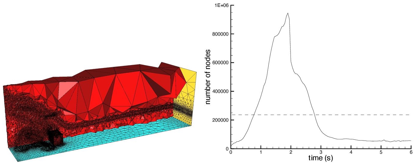
Figure 2.9. 3D falling water column on a obstacle. Mesh adaptation based on the interface and moments. Left: An example of mesh used during a time subinterval, around t = 1.2s. The mesh involves ≈ 500,000 vertices. Right: Variation of the number of mesh vertices as a function of time. The dashed line represent the average number of vertices for the whole simulation ≈ 240,000 vertices. For a color version of this figure, see www.iste.co.uk/dervieux/meshadaptation2
2.6. Conclusion
This chapter presents a first transient mesh adaptation algorithm. A second algorithm is presented in Chapter 7 of this volume. Since mesh adaptation is built from a fixed point, mesh adaptation is time implicit, that is, stable and by construction adapted to the new time levels. The adaptation is designed from a control of interpolation error in momentum field together with interface representation error. For interface error control, two criteria have been introduced and discussed. Taking into account the level set curvature allows for an improved representation of corners and small details. A particular attention has been paid to the design of an adaptation algorithm with a higher order convergence rate. Time dimension is taken into account by the choice of a constant-error criterion. This means that when the flow becomes more complex with time, so does the mesh, the final accuracy being the priority.
2.7. Appendix: remarks about the adaptation of the time step
We have not addressed the complex question of the adaptation of the timestep. In many of our applications, the model is advection dominated and advanced with explicit time stepping. In that case, a simplified assumption is as follows:
The time discretization error is approximatively bounded by a constant times the space approximation error.
Therefore, minimizing the spatial error implies that the time error is somewhat minimized accordingly.
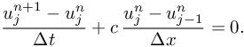
Let us give a rather heuristic proof that the above assumption is essentially verified. We analyze the error in time obtained with a first-order accurate scheme with an explicit discretization in time on the transport equation (a first-order hyperbolic problem) in one dimension:
with c > 0. Let xj for j = 1, ..., N be a uniform spatial discretization of the one-dimensional domain and let tn for n = 0, ..., T be a uniform time discretization. For each vertex xj at time tn, we have ![]() . The first-order upwind method is written
. The first-order upwind method is written
Using Taylor expansion, the local truncation error ![]() is given by
is given by
An estimation of the spatial and the time error are provided by the first and the second term, respectively (indices are omitted for clarity): ![]() and
and ![]() Applying twice the continuous equation, we get
Applying twice the continuous equation, we get ![]() therefore
therefore ![]() With CFL condition
With CFL condition ![]() this implies that the time error is bounded by the spatial error
this implies that the time error is bounded by the spatial error
This analysis extends to higher order schemes, in particular to the second-order schemes used in this book. We refer to Alauzet et al. (2007) for a more complete analysis.
2.8. Notes
The transient fixed-point mesh adaptation method was introduced in Alauzet et al. (2007). More examples of computations can be found in Guégan et al. (2010).
Dynamic adaptation with unstructured meshes dates back to previous works (Löhner 1989). Some bibliography can be found in Cao et al. (2003). Let us also refer to the monograph Adaptive Moving Mesh Methods by Huang and Russel (2011).
Notes
- 1 Let us give a short proof. Indeed, we start from a pair (ε, η) for which the adaptation to the thick interface requires Ni vertices and the adaptation to the rest of the domain, the region complementary to the thick interface where the solution is smooth, necessitates Ns vertices. Then, error threshold ε and interface thickness η are divided by four. The numbers of nodes become, respectively,
 and
and  The new smooth solution area made free by passing to a thinner interface needs a number of vertices, which is negligible with respect to the rest of the domain. Thus, the new regular region needs 2d times more vertices for an error four times smaller, according to the smooth-adaptation analysis of the previous sections
  Let us analyze the amplification
  of the number of nodes in the vicinity of the interface: thanks to the option η(ε) =Cst ε, the number of mesh layers close to interface is not changed, because the mesh size normal to the interface is four times smaller, but it is applied also in a width four times smaller. The mesh is also adapted in the direction tangent to the interface. The necessary number of nodes depends on whether the mesh adaptation is anisotropic or not. In the isotropic case, the volume to mesh is four times smaller, with a mesh step four times smaller. The number of nodes is multiplied by a factor:
  . In the anisotropic case, due to the bound concerning the interface curvature and measure, we can apply a two times smaller step in tangent direction(s), which, taking into account that the number of normal layers is constant, gives a factor
  , less than
  .
.
- 2 Anisotropic unsteady calculations are described in Chapter 7 of this volume.
- 3 Available at: http://www.marin.nl/web/show.
- 4 Available at: http://wiki.manchester.ac.uk/spheric/index.php/SPHERIC_Home_Page.
- 5 Code NiceFlow in MPI mode.
- 6 It is important to note that in MARIN pictures only a part of the domain is represented. The part of the domain where the water was initially held back by the hatch is missing. It represents one-third of the domain total length. This missing part is shown by the icon top right of the picture.