
This chapter will extend the linked list implementation to stacks and queues. Stacks and queues are special cases of linked lists with less flexibility in performing operations than linked lists. However, these data structures are easy to implement and have higher efficiency where such structures are needed. For example, Figure 1.4, in Chapter 1, Getting Started shows the implementation of an array with integer data type using stacks and queues. An item can be added (PUSH) or deleted (POP) from a stack from one side only, whereas a queue is an implementation of linear data structure, which allows two sides for insertion (enqueue) and deletion (dequeue). The current chapter will cover array-based and linked list-based implementation of stacks and queues in R. This chapter will cover below topics in detail:
- Stacks
- Array-based stacks
- Linked stacks
- Comparison of array-based and linked stacks
- Implementing recursion
- Queues
- Array-based queues
- Linked queues
- Comparison of array-based and linked queues
- Dictionaries
Stacks are a special case of linked list structures where data can be added and removed from one end only, that is, the head, also known as the top. A stack is based on the Last In First Out (LIFO) principle, as the last element inserted is the first to be removed. The first element in the stack is called the top, and all operations are accessed through the top. The addition and removal of an element from the top of a stack is referred to as Push and Pop respectively, as shown in Figure 4.1:

Figure 4.1: Example of Push and Pop operation in stacks
A stack is a recursive data structure, as it consists of a top element, and the rest is either empty or another stack. The main ADT required to build a stack is shown in Table 4.1. This book will cover two approaches-array-based stack and linked stack-to implement the ADT mentioned in Table 4.1. The implementation is covered using reference classes in R:
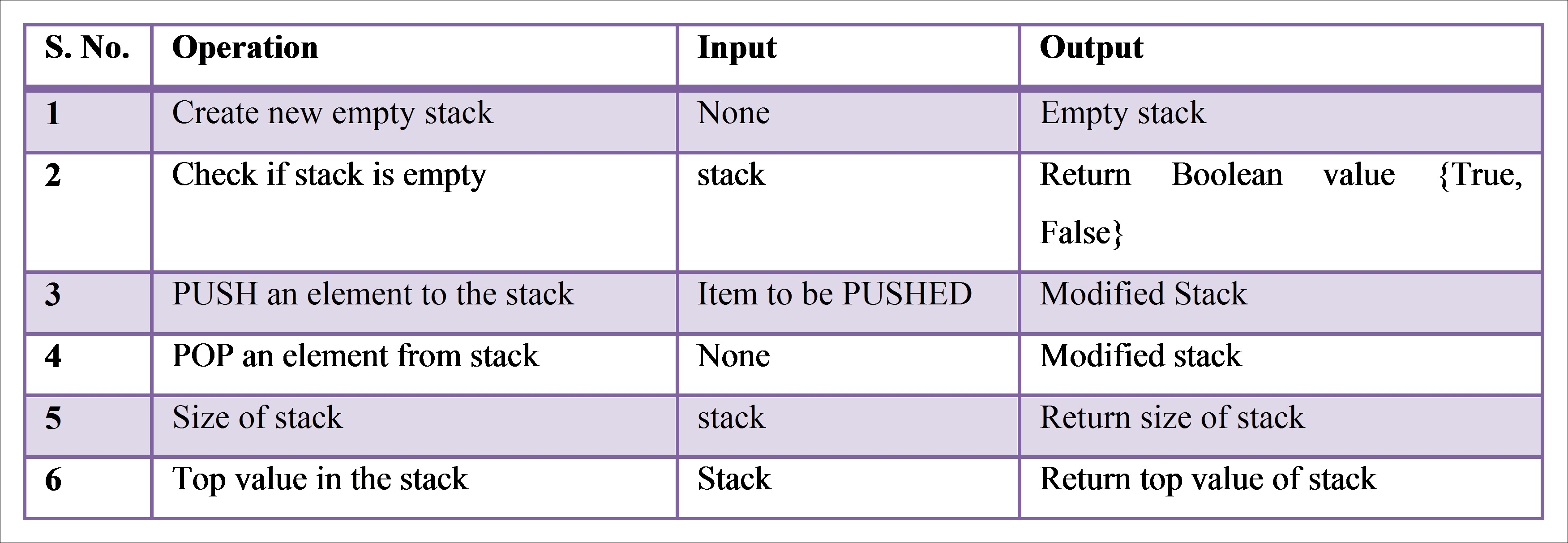
Table 4.1 Abstract data type for queue
Array-based stack implementation uses the array data structure to store data. Similar to an array-list, an array-based stack uses a fixed size. Thus, the class definition for an array-based stack would be similar to an array-based list, as shown in the following code:
Astack <- setRefClass(Class = "Astack",
  fields = list(
    Maxsize="integer",
    topPos="integer",
    ArrayStack="array"
  ),
  methods = list(
    # Initialization function
    initialize=function(defaultSize=100L,...){
      topPos<<-0L
      Maxsize<<-defaultSize # 100L
      ArrayStack<<-array(dim = Maxsize)
    },

    # Check if stack is empty
    isEmpty=function(){},

    # push value to stack
    push=function(pushval){},

    # Pop value from stack
    pop=function(){},

    # Function to get size of stack
    stacksize=function(){},

    # Function to get top value of stack
    top=function(){}
  )
)
In reference classes, fields are modified using <<- (global operator), and all functions are accessible to objects created using the defined class. The preceding class implements a stack with a default array size of 100 cells. The pointer topPos points to the top element of the stack, and Maxsize refers to the maximum size of the array. To check whether the stack is empty or not, we can use the top position in an array stack, as follows:
isEmpty=function(){
  if(topPos==0) {
    cat("Empty Stack!")
    return(TRUE)
  } else
  {
    return(FALSE)
  }
}
The push and pop operation of an array stack can be performed by working with the topPos pointer of the class to update the array index:
push=function(pushval){
  if((topPos+1L)>Maxsize) stop("Stack is OUT OF MEMORY!")
  topPos<<-topPos+1L
  ArrayStack[topPos]<<-pushval
}

pop=function(){
  # Check if stack is empty
  if(isEmpty()) return("Empty Stack!")
  popval<-ArrayStack[topPos]
  ArrayStack[topPos]<<-NA
  topPos<<-topPos-1L
  return(popval)
}
Pushing an element to a stack which is completely full is known as overflow, whereas removing an element from a stack which is empty is referred to as underflow of stack. Thus, both these conditions are added as exceptions in the current class using the isEmpty function Maxsize variable. The size of the array stack can be obtained by returning the topPos variable:
stacksize=function(){
  stackIsEmpty<-isEmpty()
  ifelse(stackIsEmpty, return(0), return(topPos))
}
Similarly, the top value of a stack can be returned by returning the value pointed to by topPos into ArrayStack:
top=function(){
  stackIsEmpty<-isEmpty()
  if(stackIsEmpty) {
    cat("Empty Stack")
  } else
  {
    return(ArrayStack[topPos])
  }
}
Due to the simplicity of the structure and implementation of stacks, it is possible to implement multiple stacks within the same initialized array. However, the current implementation is recommended if stacks have an inverse relationship, or if there is a functional relationship which could be used to minimize the array memory. For example, a two-stack system in which the first stack gets data from the pop operation performed on the second stack can be utilized to develop a multi-array stack within the same array, as shown in Figure 4.2.
In Figure 4.2, Stack1top and Stack2top represent the pointers to the first and second stacks, respectively. As Stack1top moves toward the right, Stack2top moves toward the left, and vice versa. For other scenarios where the memory required is not predefined, a linked stack can be used, as discussed in the next subsection:

Figure 4.2: Example of a multi-array stack
An example of the use of an array-based stack with multiple push and pop operations is as follows:
> array_stack_ex<- Astack$new()
> array_stack_ex$push(1)
> array_stack_ex$push(2)
> array_stack_ex$push(3)
> array_stack_ex$pop()
> array_stack_ex$push(5)
> array_stack_ex$pop()
> array_stack_ex$pop()
> array_stack_ex$top()
[1] 1
> array_stack_ex
Reference class object of class "Astack"
Field "Maxsize":
[1] 100
Field "topPos":
[1] 1
Field "ArrayStack":
[1]  1 NA NA NA NA NA NA NA ... NA NA NA
Initially, we push three elements into the stack {1, 2, 3}. We then pop one element out using the LIFO principle, and are, thus, left with the set {1,2}. We then push another element 5 into the stack, updating the set as {1,2,5}. Finally, we pop the top two elements, leaving the stack with only one element, {1}.
Linked list-based stacks utilize the concept of linked lists with the flexibility to add and remove elements dynamically from the head of a linked list, which is equivalent to the top in an array-based stack. The top points to the first member of the linked list, as shown in Figure 4.3:

Figure 4.3: A linked stack with the top pointing to the head node of a linked list
The reference class definition of a linked list-based stack is shown as follows:
Linkstack <- setRefClass(Class = "Linkstack",
  fields = list(
    Lsize="integer",
    Lstacktop="environment"),
  methods = list(
    # Initialization function
    initialize=function(...) {
      Lsize<<-0L
    },

    # Check if stack is empty
    isEmpty=function(){},

    # Function to create empty R environment
    create_emptyenv=function(){},

    # Function to create node
    Node = function(val, node=NULL) {},

    # push value to stack
    push=function(pushval){},

    # Pop value from stack
    pop=function(){},

    # Function to get top value of stack
    top=function(){}
  )
)
As nodes are created dynamically, memory allocation is not required; thus, Lstacktop is defined as an environment variable, and points to the top location of the stack. The Lsize variable stores the stack's size. The fundamental node of a linked list comprises the value and address of the next node. Let's use the same ADT as defined earlier for the array-based stack. We could utilize the same isEmpty function defined for the array stack by replacing topPos with Lsize:
isEmpty=function(){
  if(Lsize==0) {
    cat("Empty Stack!")
    return(TRUE)
  } else
  {
    return(FALSE)
  }
}
The node in the linked stack can be defined as an environment object similar to a linked list as defined in Chapter 3, Linked Lists:
create_emptyenv = function() {
  emptyenv()
}
Node = function(val, node=NULL) {
  llist <- new.env(parent=create_emptyenv())
  llist$element <- val
  llist$nextnode <- node
  llist
}
The node method consists of element, which stores the value, and nextnode, which points to next node of the linked list. The push method will add a node to the stack, whereas the pop method will remove the top node of the stack:
push=function(val){
  stackIsEmpty<-isEmpty()
  if(stackIsEmpty){
    Lstacktop<<-Node(val)
    Lsize<<-Lsize+1L
  } else
  {
    Lstacktop<<-Node(val, Lstacktop)
    Lsize<<-Lsize+1L
  }
}
The push function initially checks whether the stack is empty or not. If the stack is empty, it creates a new node, otherwise it adds the newly created node to the top position of the linked list. As accessing the top position or head node of a linked list is quite straightforward, we do not require to define a separate top variable pointing to the head node in R; thus, top is used as a reference to the head node in linked list stack definitions.
pop=function(){
  stackIsEmpty<-isEmpty()
  if(stackIsEmpty){
    cat("Empty Stack")
  } else
  {
    Lstacktop<<-Lstacktop$nextnode
    Lsize<<-Lsize-1L
  }
}
The pop function also checks for the empty condition, and moves the top position to nextnode using the address pointer if the stack is non-empty. The other functionality of stacks can be built around their basic ADT, such as getting the top value of a stack:
topVal=function(){
  stackIsEmpty<-isEmpty()
  if(stackIsEmpty){
    cat("Empty Stack")
  } else
  {
    return(Lstacktop$element)
  }
}
The preceding function returns element from the top node of a stack. This function can be used to set up a list stack. The following is an example of the use of a linked list stack with multiple push and pop operations:
> link_stack_ex<-Linkstack$new()
> link_stack_ex $push(1)
> link_stack_ex $push(2)
> link_stack_ex $push(3)
> link_stack_ex $pop()
> link_stack_ex $push(5)
> link_stack_ex $pop()
> link_stack_ex $pop()
> a$topVal()
[1] 1
> link_stack_ex

The preceding example is similar to the array-based implementation. After all the operations have been performed in this last example, array_stack_ex object has one value in the stack, as shown in the output stored in environment 0x00000000405fc248.
From the perspective of time computation, both array and linked list implementations of stacks are quite comparable. For example, the cost of appending and deleting in both arrays and linked list stacks is O(1)-worst-case. In a linked list-based implementation, appending and deletion is performed by the head pointer, which can be accessed directly. Similarly, in an array-based implementation, each push and pop is performed through the topPos index variable, which keeps moving making access in constant time.
In terms of space, in an array-based stack implementation, preallocation of memory is required during array initialization; thus, (n-m) cells are wasted, where m is the number of elements stored in the array. On the other hand, a linked list stack implementation dynamically allocates and deallocates memory with every push and pop operation respectively, and thus, no memory is wasted. However, a linked list implementation requires an extra nextnode field to store the address of the next node.
Recursion is used to implement an iterative process, where each state of a variable in a subroutine is registered by the controller. The primary memory, while executing the code, utilizes four main components, as shown in Figure 4.4:
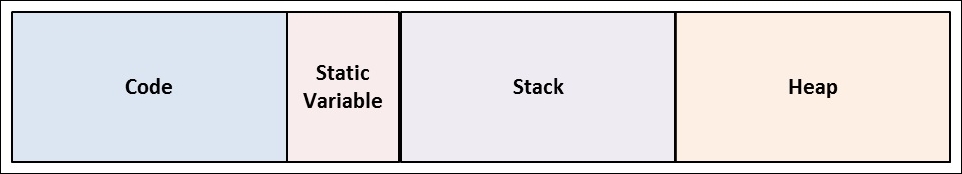
Figure 4.4: Memory allocation
The code part of the memory stores instructions and functions from the program. The static variable stores any global and static variable from the program. The stack stores the variables and data of the function. The heap is used for dynamic memory allocation. For example, a subroutine with data and instructions will register into memory, as shown in Figure 4.5. The subroutine variables x and y are stored in the Stack, whereas instructions are stored in the Code section of memory allocation. When implemented as a recursion, the machine executes a subroutine repeatedly by changing the contents of the registers until the termination condition is reached. At each step, the state of the subroutine is determined based on the register content in the stack, which comprises variable states:

Figure 4.5: Example of memory allocation
The recursive function should always have a termination criterion to be used in real-world applications. Anything which has a self-similar structure with repetition can be implemented using recursion. For example, the factorial of any non-negative integer for any number n is represented as n!, and can be expressed as follows:
factorial(n) = n*factorial(n-1) where factorial(0)=1.
The factorial function is self-similar, as it calls itself until it reaches a value factorial(0). The following represents the R implementation of factorial using recursion:
recursive_fact<-function(n) {
  if(n<0) return(-1)
  if(n == 0) {
    return(1)
  } else {
    return(n*recursive_fact(n-1))
  }
}
The preceding factorial function uses recursion for evaluation, and uses a stack for computation. For example, for the factorial of 3, the preceding function will keep pushing values to the stack until the termination condition is achieved (as shown in Figure 4.6) before calculating the factorial by popping the stored value from the stack. The function will create a stack of all the values to be multiplied before popping these values from the stack to perform the final multiplication operation to give the factorial value for the given integer:
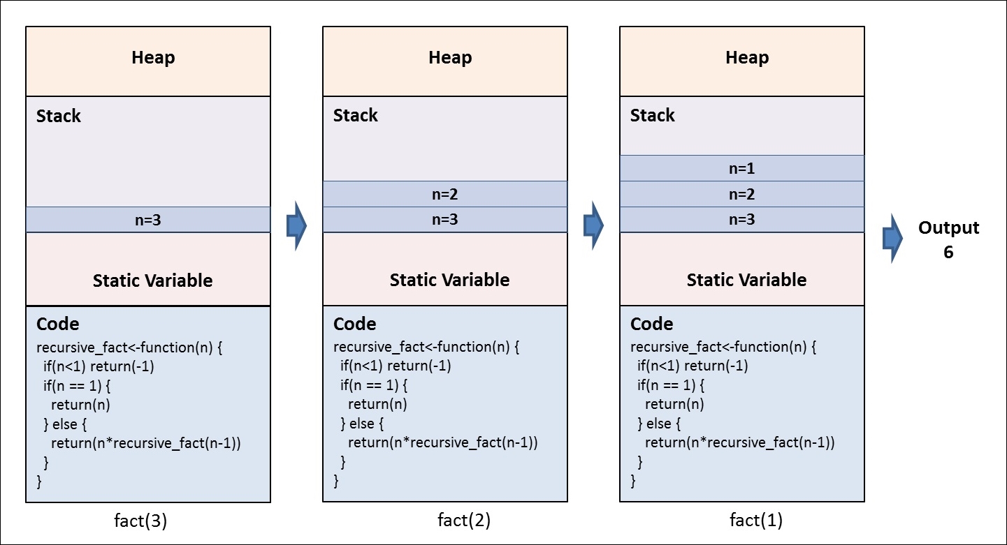
Figure 4.6: Example of recursion for factorial of 3
The recursion approaches are quite efficient in implementing algorithms that require multiple branching, such as binary trees. The details of these algorithms will be covered in a later part of this book.