
1
How to Reconstruct the History of a Digital Image, and of Its Alterations
Quentin BAMMEY1, Miguel COLOM1, Thibaud EHRET1, Marina GARDELLA1, Rafael GROMPONE1, Jean-Michel MOREL1, Tina NIKOUKHAH1 and Denis PERRAUD2
1 Centre Borelli, ENS Paris-Saclay, University of Paris-Saclay, CNRS, Gif-sur-Yvette, France
2 Technical and Scientific Police, Central Directorate of the Judicial Police, Lyon, France
Between its raw acquisition from a camera sensor and its storage, an image undergoes a series of operations: denoising, demosaicing, white balance, gamma correction and compression. These operations produce artifacts in the final image, often imperceptible to the naked eye but yet detectable. By analyzing those artifacts, it is possible to reconstruct the history of an image. Indeed, one can model the different operations that took place during the creation of the image, as well as their order and parameters.
Information about the specific camera pipeline of an image is relevant by itself, in particular because it can guide the restoration of the image. More importantly, it provides an identifying signature of the image. A model of the pipeline that is inconsistent across the whole image is often a clue that the image has been tampered with.
However, the traces left by each step can be altered or even erased by subsequent processing operations. Sometimes these traces are even maliciously masked to make a forged image seem authentic to forensic tools. While it may be easy to deliberately hide the artifacts linked to a step in the processing of the image, it is more difficult to simultaneously hide several of the artifacts from the entire processing chain. It is therefore important to have enough different tests available, each of them focused on different artifacts, in order to find falsifications.
We will therefore review the operations undergone by the raw image, and describe the artifacts they leave in the final image. For each of these operations, we will discuss how to model them to detect the significant anomalies caused by a possible manipulation of the image.
1.1. Introduction
1.1.1. General context
The Internet, digital media, new means of communication and social networks have accelerated the emergence of a connected world where perfect mastery over information becomes utopian. Images are ubiquitous and therefore have become an essential part of the news. Unfortunately, they have also become a tool of disinformation aimed at distracting the public from reality.
Manipulation of images happens everywhere. Simply removing red eyes from family photos could already be called an image manipulation, whereas it is simply aimed at making an image taken with the flash on look more natural. Even amateur photographers can easily erase the electric cables from a vacation panorama and correct physical imperfections such as wrinkles on a face, not to mention the touch-ups done on models in magazines.
Beyond these mostly benign examples, image manipulation can lead to falsified results in scientific publications, reports or journalistic articles. Altered images can imply an altered meaning, and can thus be used as fake evidence, for instance to use as defamation against someone or report a paranormal phenomenon. More frequently, falsified images are published and relayed on social media, in order to create and contribute to the spread of fake news.
The proliferation of consumer software tools and their ease of use have made image manipulation extremely easy and accessible. Some software even go as far as to automatically restore a natural look to an image when parts of it have been altered or deleted. Recently, deep neural networks have made it possible to generate manipulated images almost automatically. One example is the site This Person Does Not Exist1, which randomly generates faces of people who do not exist while being unexpectedly realistic. The most surprising application is undoubtedly the arrival of deepfake methods, which allow, among other things, a face in a video to be replaced with the one of another person (face swapping).
1.1.2. Criminal background
These new possibilities of image manipulation have been exploited for a long time by governments, criminal organizations and offenders. Stalinist propaganda images can come to mind, in which certain characters who had become undesirable were removed from official photographs (Figure 1.1).
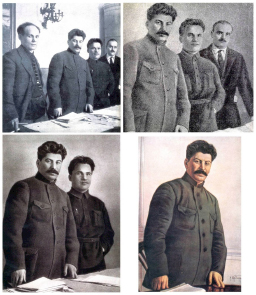
Figure 1.1. An example showing how an image has been modified several times in a row, each person who had lost favor seeing their image removed from the photo. Only Joseph Stalin appears in all four photos
Today, image manipulation can serve the interests of criminal or terrorist organizations as part of their propaganda (false claims, false events, masking of identification elements, addition of objects). Face swapping and deepfake techniques are also a simple way to undermine the image and privacy of public figures by placing them in compromising photos. The manipulation of images is also a means of exerting coercion, pressure or blackmail against a third party. These new image manipulation techniques are also used by pedophiles to generate photographs that satisfy their fantasies. Manipulated images can also be used to cause economic harm to companies through disinformation campaigns. Administrative documents can be falsified in order to obtain official papers, a rental document or a loan from specialized organizations. Face morphing, whose objective is to obtain the photo of a visually “compatible” face from two faces, enables two users to share the same ID in order to deceive an identity check.
1.1.3. Issues for law enforcement
In the past, confessions, testimonies or photographs were enough to prove guilt. Technologies were not sufficiently developed to mislead investigators. Today, these methods are no longer sufficient and law enforcement authorities need innovative scientific tools to be able to present reliable evidence in court. As technology evolves rapidly, law enforcement agencies must continuously ensure scientific monitoring in order to keep up with the state-of-the-art technology, to anticipate and to have the most recent tools available to detect manipulation and other forms of cheating for malicious purposes. It is essential to maintain a high level of training for the experts responsible for authenticating the images. In fact, the role of the police, and in particular of the technical and scientific police, is to highlight any falsification in order to allow perpetrators to be sentenced, but also to exonerate the persons under judicial enquiry if they are innocent or if their crime cannot be proven. The role of the expert in image authentication is to detect any form of manipulation, rigging or editing aimed at distorting reality. They must be able to answer the following questions:
- – Is the image real?
- – Does it represent the real scene?
- – What is the history of the image and its possible manipulations?
- – What is the manipulated part?
- – Has the image come from the device that supposedly took it?
In general, it is easier to conclude that an image is falsified than to say it is authentic. Detecting manipulation traces is getting harder over time, as new forgery methods are being developed. As a result, not finding any forgery traces does not prove the image’s authenticity. The level of expertise of the forger should also be taken into account. In fact, the possible traces of manipulation will not be the same depending on whether the author is a neophyte, a seasoned photographer or a special effects professional. The author can also use so-called anti-forensic techniques aimed at masking traces of manipulation so that they become undetectable by experts; it is up to the expert to know these techniques and their weaknesses.
1.1.4. Current methods and tools of law enforcement
As technologies evolve over time, detection tools must also adapt. Particularly during the transition from film photography to digital images, the authentication methods that were mainly based on semantic analysis of the scene (visual analysis of defects, consistency of shadows and lighting, vanishing points) have been completed through structural and statistical analyses.
To date, available commercial tools are not helpful to the authentication of an image. Most of the time, experts need to design their own tools. This raises the concern of deciding on what ground results from such tools should be accepted as evidence in court. In order to compensate for this lack of objective and precise tools, the police recruits trainees, who participate in national projects (DEFALS challenge funded by the DGA and the French National Research Agency) or international projects (H2020 projects of the European Commission). The objective is to involve university researchers as well as industrialists and practitioners (forensic experts). In addition, experts develop good practice guides such as the “Best Image Authentication Practice Manual” within the framework of the ENFSI2 to standardize and formalize analysis methodologies.
Digital images are an essential medium of communication in today’s world. People need to be able to trust this method of communication. Therefore, it is essential that news agencies, governments and law enforcement maintain and preserve trust in this essential technology.
1.1.5. Outline of this chapter
Our objective is to recognize each step of the production chain of an image. This information can sometimes appear in the data accompanying the image, called EXIF (Exchangeable Image File Format), which also includes information such as the brand and model of the camera and lens, the time and location of the photograph, and its shooting settings. However, this information can be easily modified, and is often automatically deleted by social media for privacy reasons. Therefore, we are interested in the information left by the operations on the image itself rather than in the metadata. Some methods, like the one presented in Huh et al. (2018), offer to check the consistency of the data present in the image with its EXIF metadata.
Knowledge of the image production chain allows for the detection of changes.
A first application is the authentication of the camera model. The processing chain is specific to each device model; so it is possible to determine the device model by identifying the processing chain, as implemented in Gloe (2012) where features are used to classify photographs according to their source device. More recently, Agarwal and Farid (2017) showed that even steps common to many devices, such as JPEG compression, sometimes have implementation differences that allow us to differentiate models from multiple manufacturers, or even models from the same manufacturer.
Another application is the detection of suspicious regions in an image, based on the study of the residue – sometimes called noise – left by the processing chain. This residue is constituted of all the traces left by each operation. While it is often difficult, or even impossible, to distinguish each step in the processing chain individually, it is easier to distinguish two different processing chains as a whole. Using this idea, Cozzolino and Verdoliva proposed to use steganography tools (see Chapter 5 entitled “Steganography: Embedding data into Multimedia Content”) to extract the image residue (Cozzolino et al. 2015b). Treating this residue as a piece of hidden information in the image, an algorithm such as Expectation–Maximization (EM) is then used to classify the different regions of the image. Subsequently, neural networks have shown good performance in extracting the residue automatically (Cozzolino and Verdoliva 2020; Ghosh et al. 2019), or even in carrying out the classification themselves (Zhou et al. 2018).
The outline of this chapter arises from previous considerations. Section 1.2 describes the main operations of the image processing chain.
Section 1.3 is dedicated to the effect each step of the image processing pipeline has on the image’s noise. This section illustrates how and why the fine analysis of noise enables the reverse engineering of the image and leads to the detection of falsified areas because of the discrepancies in the noise model.
We then detail the two main operations that lead to the final coding of the image. Section 1.4 explains how demosaicing traces can be detected and analyzed to detect suspicious areas of an image. Section 1.5 describes JPEG encoding, which is usually the last step in image formation, and the one that leaves the most traces. Similarly to demosaicing, we show how the JPEG encoding of an image can be reverse-engineered to understand its parameters and detect anomalies. The most typical cases are cropping and local manipulations, such as internal or external copy and paste.
Section 1.6 specifically addresses the detection of internal copy-move, a common type of manipulation. Finally, section 1.7 discusses neural-network-based methods, often efficient but at the cost of interpretability.
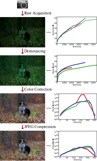
Figure 1.2. Simplified processing pipeline of an image, from its acquisition by the camera sensor to its storage as a JPEG-compressed image. The left column represents the image as it goes through each step. The right column plots the noise of the image as a function of intensity in all three channels (red, green, blue). Because each step leaves a specific footprint on the noise pattern of the image, analyzing this noise enables us to reverse engineer the pipeline of an image. This in turn enables us to detect regions of an image which were processed differently, and are thus likely to be falsified
1.2. Describing the image processing chain
The main steps in the digital image acquisition process, illustrated in Figure 1.2, will be briefly described in this section. Other very important steps, such as denoising, are beyond the scope of this chapter and will therefore not be covered here.
1.2.1. Raw image acquisition
The first step of acquiring a raw image consists of counting the number of incident photons over the sensor along the exposure time. There are two different technologies used in camera sensors: charge coupled devices (CCDs) and complementary metal-oxide-semiconductors (CMOS). Although their operating principles differ, both can be modeled in a very similar way (Aguerrebere et al. 2013). Both sensors transform incoming light photons into electronic charge, which interacts with detection devices to produce electrons stored in a potential light well. When the latter is full, the pixels become saturated. The final step is to convert the analog voltage measurements into digital quantized values.
1.2.2. Demosaicing
Most cameras cannot see color directly, because each pixel is obtained through a single sensor that can only count the number of photons reaching it in a certain wavelength range. In order to obtain a color image, a color filter array (CFA) is placed in front of the sensors. Each of them only counts the photons of a certain wavelength. As a result, each pixel has a value relative to one color. By using filters of different colors on neighboring pixels, the missing colors can then be interpolated.
Although others exist, almost all cameras use the same CFA: the Bayer array, which is illustrated in Figure 1.3. This matrix samples half the pixels in green, a quarter in red and the last quarter in blue. Sampling more pixels in green is justified by the human visual system, which is more sensitive to the color green.
Unlike other steps in the formation of an image, a wide variety of algorithms are used to demosaic an image. The most simple demosaicing algorithm is bilinear interpolation: missing values are interpolated by averaging the most direct neighbors sampled in that channel. As the averaging is done regardless of the image gradient, this can cause visible artifacts when interpolated against a strong gradient, such as on image edges.
To avoid these artifacts, more recent methods attempt to simultaneously take into account information from the three color channels and avoid interpolation along a steep gradient. For instance, the Hamilton–Adams method is carried out in three stages (Hamilton and Adams 1997). First, it interpolates the missing green values by taking into account the green gradients corrected for the discrete Laplacian of the color already known at each pixel to interpolate horizontally or vertically, in the direction where the gradient is weakest. It then interpolates the red and blue channels on the pixels sampled in green, taking the average of the two neighboring pixels of the same color, corrected by the discrete Laplacian of the green channel in the same direction. Finally, it interpolates the red channel of blue-sampled pixels and the blue channel of red-sampled pixels using the corrected average of the Laplacian of the green channel, in the smoothest diagonal.
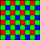
Figure 1.3. The Bayer matrix is by far the most used for sampling colors in cameras
Linear minimum mean-square error demosaicing (Getreuer 2011) suggests working not directly on the three color channels (red, green and blue), but on the pixelwise differences between the green channel and each of the other two channels separately. It interpolates this difference separately in the horizontal and vertical directions, in order to estimate first the green channel, followed by the differences between red and green, and then between blue and green. The red and blue channels can then be recovered by a simple subtraction. This method, as well as many others, makes the underlying assumption that the difference of color channels is smoother than the color channels themselves, and therefore easier to interpolate.
More recently, convolutional neural networks have been proposed to demosaic an image. For instance, demosaicnet uses a convolutional neural network to jointly interpolate and denoise an image (Gharbi et al. 2016; Ehret and Facciolo 2019). Even if these methods offer superior results to algorithms without training, they also require more resources, and are therefore not widely used yet in digital cameras.
The methods described here are only a brief overview of the large array of methods that exist for image demosaicing. This variety is increased by the fact that most industrial cameras do not disclose their often private demosaicing algorithm.
No demosaicing method is perfect – after all, it is a matter of reconstructing missing information – and produces some level of artifacts, although some produce much fewer artifacts than others. Therefore, it is possible to detect these artifacts to obtain information on the demosaicing method applied to the image, which is explained in section 1.4.
1.2.3. Color correction
White balance aims to adjust values obtained by the sensors, so that they match the colors perceived by the observer by adjusting the gain values of each channel. White balance adjusts the output using characteristics of the light source, so that achromatic objects in the real scene are rendered as such (Losson and Dinet 2012).
For example, white balance can be achieved by multiplying the value of each channel, so that a pixel that has a maximum value in each channel is found to have the same maximum value 255 in all channels.
Then, the image goes through what is known as gamma correction. The charge accumulated by the sensor is proportional to the number of photons incident on the device during the exposure time. However, human perception is not linear with the signal intensity (Fechner 1860). Therefore, the image is processed to accurately represent human vision by applying a concave function of the form ![]() , where γ typically varies between 1.8 and 2.2. The idea behind this procedure is not only to enhance the contrast of the image but also to encode more precisely the information in the dark areas, which are too dark in the raw image.
, where γ typically varies between 1.8 and 2.2. The idea behind this procedure is not only to enhance the contrast of the image but also to encode more precisely the information in the dark areas, which are too dark in the raw image.
Nevertheless, commercial cameras generally do not apply this simple function, but rather a tone curve. Tone curves allow image intensities to be mapped according to precomputed tables that simulate the nonlinearity present in human vision.

Figure 1.4. JPEG compression pipeline
1.2.4. JPEG compression
The stages of the JPEG compression algorithm, illustrated in Figure 1.4, are detailed below. The first stage of the JPEG encoding process consists of performing a color space transformation from RGB to YCBCR, where Y is the luminance component and CB and CR are the chrominance components of the blue difference and the red difference. Since the Human Visual System (HVS) is less sensitive to color changes than to changes in luminance, color components can be subsampled without affecting visual perception too much. The subsampling ratio generally applied is 4:2:0, which means that the horizontal and vertical resolution is reduced by a factor of 2. After the color subsampling, each channel is divided into blocks of 8 × 8 and each block is processed independently. The discrete cosine transform (DCT) is applied to each block and the coefficients are quantized.
The JPEG quality factor Q, ranging between 1 and 100, corresponds to the rate of image compression. The lower this rate, the lighter the resulting file, but the more deteriorated the image. A quantization matrix linked to Q provides a factor for each component of the DCT blocks. It is during this quantization step that the greatest loss of information occurs, but it is also this step that allows the most space in memory to be saved. The coefficients corresponding to the high frequencies, whose variations the HVS struggles to distinguish, are the most quantized, sometimes going so far as to be entirely canceled.
Finally, as in the example in Figure 1.5, the quantized blocks are encoded without loss to obtain a JPEG file. Each 8 × 8 block is zig-zagged and the coefficients are arranged as a vector in which the first components represent the low frequencies and the last ones represent the high frequencies.
Lossless compression by RLE coding (range coding) then exploits the long series of zeros at the end of each vector due to the strong quantization of the high frequencies, and then a Huffman code allows for a final lossless compression of the data, to which a header is finally added to form the file.
1.3. Traces left on noise by image manipulation
1.3.1. Non-parametric estimation of noise in images
Noise estimation is a necessary preliminary step to most image processing and computer vision algorithms. However, compared to the literature on denoising, research on noise estimation is scarce (Lebrun et al. 2013). Most homoscedastic white noise estimation methods (Lee 1981; Bracho and Sanderson 1985; Donoho and Johnstone 1995, 1994; Immerkær 1996; Mastin 1985; Voorhees and Poggio 1987; Lee and Hoppel 1989; Olsen 1993; Rank et al. 1999; Ponomarenko et al. 2007) follow the same paradigm: they look for flat regions in the image and estimate noise in high frequencies, where noise dominates over signal.
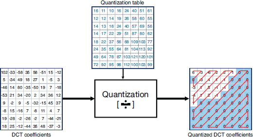
Figure 1.5. An example of the impact of quantization on a DCT block. Each DCT coefficient is quantized by a value found in a quantization matrix. Rounding to the nearest integer results in many of the high-frequency coefficients being set to zero. Each block is zig-zagged to be encoded as a vector with a sequence of zeros
We shall limit ourselves to discuss the method acknowledged as the best estimator for homoscedastic noise in the review (Lebrun et al. 2013), the Ponomarenko et al.’s method (Ponomarenko et al. 2007). This method computes the variance of overlapping 8 × 8 pixels blocks. To avoid the effects of textures and edges, blocks are sorted according to their low-frequency energy; only a small percentile (typically 0.5%) is used to select the blocks whose low- and medium-frequency energy is lowest. The final noise estimation is obtained by computing the median of the variances in the high frequencies of these blocks.
Homoscedastic white noise estimation algorithms can be adapted to estimate an arbitrary signal-dependent noise curve, as pointed out by Colom et al. (2014). However, after undergoing the complete camera processing chain detailed in section 1.3.2, noise depends not only on signal but also on frequency. A multi-scale estimation is needed in order to estimate highly correlated frequency-dependent noise (Lebrun et al. 2015). Following this observation, Colom and Buades extended Ponomarenko et al.’s method (Ponomarenko et al. 2007) to incorporate such a multi-scale approach (Colom and Buades 2013).
1.3.2. Transformation of noise in the processing chain
This section examines the way in which noise is affected at each step of the camera processing chain (see section 1.2). Noise curves obtained with the extended Ponomarenko et al.’s method (Colom and Buades 2013) along the processing chain (raw image, demosaicing, white balance, gamma correction and JPEG-encoding) are presented in Colom (2014) and compared to the temporal estimation.
Temporal estimations of noise curves are non-parametric, and good enough to be considered as ground-truth. Having ground-truth noise curves is an important issue when evaluating the performance of estimation methods. These temporal estimations are built by taking burst photos of the same scene, which consists of a calibration pattern with large flat zones (Figure 1.6), under constant lighting with a steady camera. Under these conditions, the variance of a pixel value can only be explained by noise. Thus, the noise curve obtained by computing the standard deviation of the temporal series yields the ground-truth noise curve. These noise curves depend on the camera used as well as the particular processing chain, including the ISO level and the exposure time.
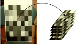
Figure 1.6. Calibration model used for the construction of the temporal series
1.3.2.1. Raw image acquisition
The value at each pixel generated by the process described in section 1.2.1 can be modeled as a Poisson variable, whose expectation is the real value of the pixel. The noise measured at the CCD or CMOS sensor has several components; Table 1.1 describes the main sources.
Figure 1.2 shows the noise curve obtained by temporal series (ground truth) and the estimation obtained from a single image computed using Ponomarenko et al.’s method (Colom and Buades 2013) with a simplified pipeline. Note that the estimate is accurate since all curves match. At this step, all channels have the same noise curve. As noise follows a Poisson distribution, the noise variance follows a simple linear relation σ2 = a + bu, where u is the intensity of the ideal noiseless image, and a and b are constants. Consequently, the noise curves are strictly increasing. Moreover, although the noise curves do not account for it, the noise characteristics reported above suggest that the noise is uncorrelated, that is, the noise at a certain pixel is not related to noise at any other pixel with the same signal intensity.
Table 1.1. Description of the main sources of noise during the acquisition process
| Type of noise | Description |
|---|---|
| Shot noise | Due to the physical nature of light. It describes the fluctuations in the number of photons detected due to their independent emission from each other. |
| Dark noise | Some electrons accumulate on the potential well as the result of a thermal cause. These electrons are known as dark current because they are present and will be detected even in the absence of light. |
| Photo response non-uniformity (PRNU) | It describes the way in which the individual pixels in the sensor array respond to uniform light sources. Due to variations in pixel geometry, substrate material, and micro-lenses, different pixels do not produce the same number of electrons from the same number of photons hitting them. |
| Readout noise | During the readout phase of the acquisition process, a voltage value is read at each pixel. This voltage is computed as a potential difference from a reference level which represents the absence of light. Thermal noise, inherent in the readout circuit, affects the output values. |
| Electronic noise | It is caused by the absorption of electromagnetic energy by the semiconductors of the camera circuits and the cross-talk phenomenon. |
1.3.2.2. Demosaicing
Demosaicing is presented in more detail in section 1.2.2. After this step, the noise at each pixel is correlated with its neighbors. After demosaicing, each channel has a different noise curve since channels are processed differently by the demosaicing algorithm.
In addition, the noise curves calculated using Ponomarenko et al.’s method and those obtained from the temporal series no longer match. This is due to the fact that Ponomarenko et al.’s algorithm assumes white noise and estimates noise at high frequencies, which are affected by demosaicing. As the image processing chain is sequential, the temporal noise curves and those measured on a single image will no longer match after demosaicing.
1.3.2.3. Color correction
White balance increases the intensity range of the image. Since the weights are different for each color channel, as mentioned in section 1.2.3, the three noise curves are less correlated after this step. Then, gamma correction greatly increases the noise and the dynamic range of the image, due to the power law function. Furthermore, the noise curves are no longer monotonically increasing after this step. Indeed, if we denote γ the function applied during the gamma correction step, the asymptotic expansion around the intensity u yields γ(u + n) = γ(u) + γ′(u)n, where n is the noise at the intensity u.
1.3.2.4. JPEG compression
The dynamic range remains unchanged after JPEG compression. However, noise is reduced after JPEG compression due to the quantization of the DCT coefficients, in particular those corresponding to high frequencies. Furthermore, the curve estimated by Ponomarenko et al.’s algorithm (Colom and Buades 2013) differs more from the temporal series curves, because the noise estimation method estimates noise at high frequencies, which are altered or even destroyed by compression.
The noise present in JPEG images is the result of several transformations on the initial noise model, which initially follows a Poisson distribution. In the end, the final image’s noise does not follow any predefined model, it instead depends on many unknown parameters that are set by each manufacturer. The only certainty we have is that noise is intensity dependent and frequency dependent. Therefore, it is preferable to use non-parametric models to estimate noise curves, so as to estimate the curves from the image itself.
1.3.3. Forgery detection through noise analysis
Image tampering, such as external copy–paste (splicing) or internal texture synthesis, can be revealed by inconsistencies in local noise levels, since noise characteristics depend on lighting conditions, camera sensors, ISO setting, and post-processing, as shown in section 1.3.2.
One of the unique features characterizing noise is the photographic response non-uniformity (PRNU), as presented in section 1.3.2. Chen et al. propose to detect the source digital camera by estimating the PRNU (Chen et al. 2008). According to the authors, the PRNU represents a unique fingerprint of image sensors and, hence, it would reveal altered images.
One of the most popular algorithms for detecting splicing using noise level traces is proposed by Mahdian and Saic (2009). It consists of dividing the image into blocks and estimating the noise level using wavelets in each block. Blocks are then merged into homogeneous regions, the noise standard deviation being the homogeneity condition. The output of this method is a map showing the segments of the image having a similar noise standard deviation.
A different approach is introduced in Pan et al. (2011), where the noise estimation is based on the kurtosis concentration phenomenon. The kurtosis of natural images across different frequency bands is constant. This allows for the estimation of noise variance when it follows an additive white Gaussian noise (AWGN) model. The method then segments the image into regions based on their noise variance using the k-means algorithm.
The method presented in Yao et al. (2017) makes use of the signal dependency of noise. Instead of a single noise level, it estimates a noise-level function. The image is segmented into edges and flat regions. It estimates the noise level on flat regions and the camera response function (CRF) on edges. Noise level functions are then compared and an empirical threshold is set to detect the salient curves. The main disadvantage of this method is that it assumes that the image has only undergone demosaicing.
We will now describe a recent method based on multi-scale noise analysis for the detection of tampering in JPEG-compressed images. After the complete camera processing chain, noise is not only signal dependent but also frequency dependent, which is mainly due to the correlation introduced by demosaicing and the quantization of DCT coefficients during JPEG compression. In this context, a multi-scale approach is necessary to capture the noise in the low frequencies. Indeed, when successive subscales are considered, the low frequencies become high frequencies due to the contraction of the DCT domain, which makes it possible to estimate the noise in low frequencies with the methods presented in section 1.3.1. One could argue that the noise contained in the low and medium frequencies could be directly estimated without considering subscales, but this is a risky procedure since these frequencies also contain part of the signal. This problem is avoided by the proposed method because, at each scale, the algorithm finds blocks having low variance in the low and medium frequencies to estimate the noise.
Consider the operator S that tessellates the image into sets of blocks of 2 × 2 pixels, and replaces each block by a pixel whose value is the average of the four pixels. We define the nth scale of an image u, and we denote it by Sn, as the result of applying n times the operator S to the image u.
The first step of the method consists of splitting the image into blocks of 512 × 512 with 1/2 overlap, which are called macro-blocks. Noise curves are estimated using Ponomarenko et al.’s method (Colom and Buades 2013) in each of the three RGB channels for each macro-block, as well as for the complete image (global estimation), at scales 0, 1 and 2. For each scale and channel, the noise curves obtained from each macro-block are compared to the global estimation.
Ideally, a non-forged image should exhibit the same noise level function for all of its macro-blocks, as well as for the entire image. However, when estimating noise curves in the presence of textures, noise overestimation is likely to happen (Liu et al. 2006). Therefore, textured macro-blocks are expected to give higher noise levels, even when they are not tampered with. Thus, the global estimation obtained provides, in fact, a lower bound for the noise curves of the individual macro-blocks. Therefore, any macro-block with lower noise levels than the global estimation is suspicious, as it would be an indicator that the underlying region has a different noise model than the rest of the image.
For detection purposes, we consider the percentage of bins in the noise curve of the macro-block whose count is below the global estimation, independently for each RGB channel and for each scale. The geometric mean of percentages obtained for each channel provides a heat map, unique to each scale. These heat maps show macro-blocks with noise levels that are incompatible with the global estimation, at a given scale.
Different criteria can be considered to define detections. One possibility is to consider that a macro-block is detected if, at any scale, the geometric mean of the percentage of cells below the overall image curve is 100%. This means that the noise curve calculated by the macro-block, at a certain scale, is entirely below the noise curve of the overall image, for all three RGB channels.
The size of the macro-blocks may appear to be too big compared to other methods willing to detect forgeries by noise analysis. This choice is made in order to achieve S2 with a reasonable number of bins to obtain an accurate enough estimation. Each sub-scale implies a reduction of the image by a factor of 2 in each direction. In this way, if the macro-blocks are 512 × 512 in S0, in S1, they are 256 × 256, and in S2, the macro-blocks are 128 × 128.
Figure 1.7 shows an example of an image where an external copy–paste has been performed. The vase on the right has been cropped from the auxiliary image and pasted onto the original image. The results of applying the proposed method to this forged image are shown in Figure 1.8.
At S0, the results do not show any different behavior in the tampered zone. If another scale is considered, S1, we find that the manipulated area has lower noise levels than the rest of the image. In fact, the noise curves corresponding to macro-blocks containing the spliced region have about 80% of their bins below the global noise curve, this percentage being slightly different for each channel. Finally, S2 provides the strongest proof of falsification. Indeed, the noise curves corresponding to forged macro-blocks have all of their bins below the global estimation in all the three RGB channels.
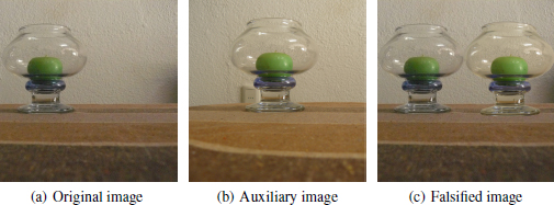
Figure 1.7. Example of falsification: the vase in b) has been cut out and copied onto a), which gives c)
COMMENT ON FIGURE 1.7.– The original image was taken with ISO 800 and exposure time 1/8 s. The auxiliary image was taken with ISO 100 and exposure time 1.3 s. Both images were taken with the same Panasonic Lumix DMC-FZ8 camera under the high-quality JPEG compression setting.
This example illustrates the need for a multi-scale approach for noise inconsistency analysis applied to forgery detection.
To conclude, noise inconsistency analysis is a rich source for forgery detection due to the fact that forged regions are likely to present different noise models from the rest of the image. However, to exploit this, it is necessary to have algorithms that are capable of dealing with signal and frequency-dependent noise. The multi-scale approach is shown as an appropriate framework for noise inconsistency analysis.
1.4. Demosaicing and its traces
Image demosaicing, which will be presented in detail in section 1.2.2, leaves artifacts that can be used to find falsifications. The Bayer CFA (see Figure 1.3) is by far the most commonly used. Mosaic detection algorithms thus focus on this matrix, although they could be adapted to other patterns.
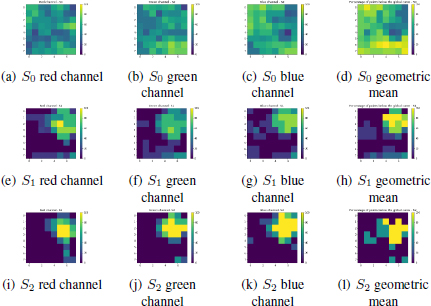
Figure 1.8. Percentage of points below the global noise curve and geometric mean for each macro-block at S0, S1 and S2
1.4.1. Forgery detection through demosaicing analysis
Detecting demosaicing artifacts can answer two questions:
- – Is it possible that a given image was obtained with a given device?
- – Is there a region of the image whose demosaicing traces are inconsistent with the rest of the image?
Two different approaches can be used to study the demosaicing of an image. One could try to estimate the specific demosaicing algorithm that was used in the image. Such an estimation might prove that an image was not taken by a given camera, assuming the demosaicing method is different from the one used by the camera. Within an image itself, a region that was demosaiced differently than the global image is likely to be forged. Such an analysis could be justified by the large variety of demosaicing methods, however this variety also limits the potential detection. To establish or disprove the link between an image and a camera through the demosaicing algorithm would require us to know the algorithm used, which is rarely the case. Estimating the specific demosaicing algorithm used by a camera would require a large amount of images from said cameras; while theoretically possible, no such work has ever been attempted. The ability to detect regions of an image that have been demosaiced with a different algorithm than the rest of the image is only theoretical; in practice the estimation of a demosaicing method once again requires more data than can usually be provided by a small region of an image. Furthermore, most demosaicing algorithms do not interpolate all regions in the same way. As a consequence, a reliable comparison of two estimations is difficult, as the same algorithm may have interpolated two regions differently. That being said, global learning-based methods can make use of the demosaicing algorithm to get information on an image, although this is just one feature learned and used among others, and not something that is conclusive by itself. For instance, Siamese-like networks such as Noiseprint (Cozzolino and Verdoliva 2020) implicitly learn some information on the demosaicing algorithm to detect forgeries. These methods will be presented in more detail in section 1.7.
A more promising approach is to directly detect the position of the Bayer matrix. Indeed, while the CFA pattern is almost always a Bayer matrix, the exact position of the matrix, that is, the offset of the CFA, varies. Detecting the position of the matrix therefore has two uses:
- – we can compare the position of the Bayer matrix in the image to the one normally used by a specific device. If the positions do not correspond, then the image was either not taken by that device, or it was cropped in the processing;
- – in the case of copy-move, both internal and external (splicing), there is a
 probability that the position of the Bayer matrix does not correspond between the original image and the pasted region. Therefore, detecting the position of the Bayer matrix, both globally and locally, can be used to find inconsistencies.
Most current demosaicing detection methods focus on this second idea, as local CFA inconsistencies give useful information on the image and can be found relatively easily in ideal conditions, that is, in uncompressed images, as we will now present.
1.4.2. Detecting the position of the Bayer matrix
Different methods make it possible to detect either the position of the Bayer matrix directly or inconsistencies of this matrix in the image.
1.4.2.1. Joint estimation of the sampled pixels and the demosaicing algorithm
In a pioneering paper on demosaicing analysis, Popescu and Farid (2005) propose to jointly estimate a linear model for the demosaicing algorithm and detect which pixels have been sampled in a given channel with an expectation-maximization (EM) algorithm. The demosaicing algorithm is estimated on pixels detected as interpolated (i.e. not sampled) as a linear combination of neighboring pixels in that channel. Sampled pixels are detected as pixels where the linear combination yields a result far from the correct value of the pixel. A pseudo-probability map of each pixel being sampled is then computed. Assuming the linear model is correct, sampled pixels will be correctly detected and there will be a strong 2-periodicity of the map, which can easily be seen as a peak in the Fourier transform of the image. However, in a region which has been altered, the estimated linear model will no longer be correct, either because the demosaicing estimation appears differently or because there are no demosaicing traces left at all. The 2-periodicity peak will thus locally disappear, and can be detected as potential evidence of a forgery. This method can then potentially classify the used demosaicing algorithm, or detect the absence of demosaicing artifacts, sign of manipulations such as blurring or inpainting to hide data on the image. To detect a change in the position of the Bayer matrix, (González Fernández et al. 2018) use a DCT instead of a Fourier transform. This simple modification enables one to directly visualize a change of position as a local change of signs at the observed peaks, instead of a harder-to-visualize phase difference. Unfortunately, while these detections were possible when Popescu’s article was first published, the demosaicing algorithms have become much more complex since then, both thanks to theoretical progress and increased computational power in cameras. Modern demosaicing algorithms process channels jointly and are strongly nonlinear, preventing an easy modelization of the demosaicing process.
1.4.2.2. Double demosaicing detection
Another method proposes to directly detect the CFA pattern used in the image (Kirchner 2010). In order to do this, the image is remosaiced and demosaiced in the four possible positions, with a simple algorithm such as bilinear interpolation. The reasoning is that demosaicing should produce an image closer to the original when it is remosaiced in the correct position. They then compare the residuals to detect which position of the CFA has been used. Since CFA artifacts are generally more visible in the green channel, they decide first the position of the sampled green pixels, before deciding between the remaining two positions with the red and blue channels, a paradigm that has been used in most publications since then. Their use of the bilinear algorithm limits them in the same way (Popescu and Farid 2005; González Fernández et al. 2018) due to the linearity and chromatic independence of the bilinear algorithm, which is not shared by most modern demosaicing algorithms. However, their method does not depend on the choice of algorithm, and could therefore provide very good results should the originally used demosaicing algorithm be known.
1.4.2.3. Direct detection of the grid by intermediate values
In order to break away from a specific algorithm, Choi et al. (2011) highlights that pixels are more likely to present extreme values locally in the channel in which they are sampled and, on the contrary, to take on intermediate values when they are interpolated (Choi et al. 2011). Therefore, they count the number of intermediate values in the four positions to decide which position is the correct one. The idea that pixels are more likely to take extreme values in their sampled channel is generally true with most algorithms, which makes this method produce good classification scores. However, the probability bias can be reversed when the algorithms make heavy use of the high frequencies of other channels, which can lead to confident, but incorrect detection of certain regions of the image.
1.4.2.4. Detecting the variance of the color difference
Shin et al. (2017) attempts to avoid the assumption that color channels are processed independently. Instead of working separately with each channel, as was done until then, they work on the difference between the green and red channels, as well as between the green and blue channels. This reflects more accurately the operations done by many demosaicing algorithms, which first interpolate the green channel before using the green channel’s information to interpolate the red and blue channels. They compute the variance of these differences in the four possible patterns on the two computed maps, and identify the correct pattern as the one featuring the highest variance, which is expected of the original pattern, whose pixels are all sampled instead of interpolated. Although the dependence of the color channels is hard-coded, the color difference is actually used in many current algorithms and represents a first step toward a full understanding of demosaicing artifacts.
1.4.2.5. Detection by neural networks of the relative position of blocks
More recently, Bammey et al. (2020) proposed to train a self-supervised convolutional neural network (CNN) to detect modulo-(2, 2) position of the blocks in the image. As CNNs are invariant to translation, they need to rely on image information to detect this position. Demosaicing artifacts, and to some extent JPEG artifacts, are the only relevant information a network can use to this end. As a result, training a network to detect this position will implicitly make it analyze demosaicing artifacts. This will thus lead to a local detection of the Bayer matrix’s position. Erroneous outputs of the network are caused by inconsistencies in the image’s mosaic, and can thus be seen as traces of forgery.
This method obtains better results than previous works, and can help further analyze the forgery as different kinds of forgeries will cause different artifacts. For instance, copy-move will cause a locally consistent shift in the network’s output, whereas inpainting – usually performed by cloning multiple small patches onto the target area – may show each cloned patch detected with a different pattern. Other manipulations, such as blurring, or the copy-move of an image that features no mosaic – for instance due to downsampling – may locally remove the mosaic, and the output of the network will thus be noise like in the forged region. It is possible to achieve even better results with internal learning, by retraining the network directly on images to study. This lets the network adapt to different post-processing, most importantly to JPEG compression.
However, this method is more computationally intense than the other presented algorithms, especially when internal learning is needed. This makes it less practical to use when many images are to be analyzed.
1.4.3. Limits of detection demosaicing
Recent methods proposed by Choi et al. (2011), Shin et al. (2017) or Bammey et al. (2020) are able to analyze the mosaic of images well enough for practical applications. It is now possible to detect, even locally, the position of the Bayer matrix. Detecting the presence of demosaicing artifacts is generally easy, even though their absence is not necessarily a sign of falsification because most modern demosaicing algorithms leave little to no artifacts on easy-to-interpolate regions. However, the range of images that can be detected remains limited. Demosaicing artifacts are 2-periodic, and they reside in the highest frequencies. As a result, they are entirely lost when the image is downsampled by a factor of at least 2. More generally, image resizing will also rescale the demosaicing artifacts; even though those might not always be lost, detection methods would need to be adapted to the new frequencies of the artifacts. JPEG compression is an even more important limitation. As compression mainly drops precision on the high-frequency components of an image, demosaicing artifacts are easily lost on compressed images. To date, even the best methods struggle to analyze CFA artifacts even at a relatively high compression quality factor of 95. Internal learning presented in Bammey et al. (2020) provides some degree of robustness to JPEG compression; however, demosaicing artifact detection remains limited to high-quality images, uncompressed or barely compressed, and at full resolution. This complements well the detection of JPEG compression, which we will now present.
1.5. JPEG compression, its traces and the detection of its alterations
In this section, we seek to determine the compression history of an image. We will focus on the JPEG algorithm, which is nowadays the most common method to store images. Most cameras use this format but others exist, such as HEIF, used in particular in Apple products since 2017. HEIF is also a lossy compression algorithm and therefore leaves traces; nevertheless, these traces are different from the ones produced by JPEG. As we will see, the analysis of the JPEG coding of an image makes it possible to detect local manipulations. For this, the methods take advantage of the structured loss of information caused by this step in the processing chain.
1.5.1. The JPEG compression algorithm
In JPEG encoding, the division of the image into 8 × 8 blocks and the application of a quantization step lead to the appearance of discontinuities at the edges of these blocks in the decompressed image.
Figure 1.9 shows the blocking effect that appears after JPEG compression. Contrast enhancement allows us to clearly see the 8 × 8 blocks. The greatest loss of information is during the quantization step, explored in more detail in section 1.2.4. The blocking effect is due to quantization, depending on the Q parameter, applied on all 8 × 8 size blocks. Therefore, standard JPEG compression leaves two characteristic traces: the division into 8×8 non-overlapping blocks and the quantization, according to a quantization matrix, of the DCT coefficients. In other words, the two features to be detected from the image are:
- 1) the origin of the 8×8 grids;
- 2) the values of the quantization matrix.

Figure 1.9. Close-ups on an image before and after compression. The contrast has been enhanced to observe the JPEG artifacts, in particular the blocking effect, allowing us to see the edges of the 8 × 8 blocks
In order to authenticate an image, the previous detections must verify that (1) the origin of the grid is aligned with the top left of the image; and (2) the quantization matrix calculated from the image is similar to the one in the header of the JPEG file. If the image is not in the JPEG format (providing the header file giving the quantization matrix), then estimating this information from the image itself is even more useful as an initial analysis.
Methods by Pevny and Fridrich (2008) make it possible to detect if an image has undergone a double compression, which creates an immediate argument against the authenticity of the image. Indeed, this would imply a duplicate in the processing chain of the image.
In the following sections, grid detection and quantization matrix estimation methods are illustrated. When no detection is made, the image may be classified as not having undergone JPEG compression.
1.5.2. Grid detection
In a JPEG-compressed image, the 8 × 8 blocks are created following a regular pattern starting at the pixel in the top left of the image and therefore coinciding with an original grid (0, 0).
The aim of the method is to find the stage of separation in 8 × 8 blocks of the JPEG algorithm. This leads to having the position of the grid by giving its origin (this can vary if the image is cropped). If a grid is present, among the 8 × 8 = 64 different original possibilities, only one is correct.
Here, two families of methods are presented: methods based on block artifacts and methods based on the impact of quantization on the DCT coefficients.
1.5.2.1. Compression artifacts
These are methods based on the detectable traces left by compression. In their article, Minami and Zakhor propose a way of detecting JPEG grids with the aim of removing the blocking artifacts (Minami and Zakhor 1995). Later on, in Fan and de Queiroz (2003), the same ideas are used to decide whether an image has undergone JPEG compression, depending on whether traces are present or not. These methods use filters to bring out the traces of compression (Chen and Hsu 2008; (Li et al. 2009)). The simplest method calculates the absolute value of the gradient magnitude of the image (Lin et al. 2009), and others use the absolute value of derivatives of order 2 (Li et al. 2009). However, these two filters can have a strong response to edges and to textures present in the image and therefore can sometimes lead to faulty grid detections. To reduce the interference of details in the scene, a cross-difference filter, proposed by Chen and Hsu (2008), is more suitable. This filter, represented in Figure 1.10, amounts to calculating the absolute value of the result of a convolution of the image by a 2 × 2 kernel. The grid becomes visible because of the differentiating filter applied to the compressed image. The stronger the compression, the more this feature is present.
Recently, methods like the one proposed in Nikoukhah et al. (2020) have made these methods automatic and unsupervised thanks to statistical validation.
1.5.2.2. DCT coefficients
These are methods based on the impact of compression on the DCT coefficients. After quantization, the compression makes the size of the image file smaller by setting many of the DCT values to zero. As illustrated in Figure 1.5, the quantization leads to setting a lot of the high-frequency coefficients to zero. The values of the quantization matrix are generally larger in high frequencies. The stronger the compression, the more values are set to zero.
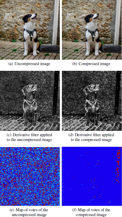
Figure 1.10. Derivative filter and vote map applied to the same image without compression in a) and after JPEG compression of quality 80 in b)
COMMENT ON FIGURE 1.10.– The compressed image features a grid structure. The saturated zone on the right of the image hides any traces of compression. In the vote map, each pixel is associated with the grid for which it voted, in other words, the grid with the most zeros. For the compressed image, one color is dominant: it corresponds to the position (0, 0).
Based on the example of CAGI (Iakovidou et al. 2018), the ZERO method determines the origin of the grid by testing the 64 possibilities and selecting the one on which the DCT coefficients of the blocks has the most zeros (Nikoukhah et al. 2019). In other words, given an image, all of its pixels vote for the grid they think they belong to. In the event of a tie, the vote is not taken into account.
Figures 1.10(e) and 1.10(f) present the vote map: each pixel’s color represents which of the 64 possible grids the pixel notes. Navy blue corresponds to the original grid (0, 0), and red to a non-valid vote, in the event of a tie. At the top right of the image, the saturated zone is not used to detect JPEG traces since it does not contain any information.
The derivative filter presented in Figures 1.10(c) and 1.10(d) makes it possible to highlight the compression artifacts, and the vote map presented in Figures 1.10(e) and 1.10(f) is a colormap where each color is associated with a grid origin. In both cases, there is a clear difference between the image that has not undergone compression and the one which has undergone compression. In fact, these filters, which are part of the tools used by journalists and police experts today, lack a validation step. Indeed, as they are presented, users need to interpret them. It is important to understand why a filter detects one area rather than another. The goal would be to get a binary result.
In the case of an uncompressed image, no “vote” stands out significantly compared to the others. In the case of the compressed image in Figure 1.10(f), navy blue is dominant: it corresponds to position (0, 0).
Whether it is the cross-difference or the pixel vote map, some areas remain difficult to interpret, therefore justifying the need for a statistical validation. For example, the saturated parts have no visible JPEG grid and therefore cannot be used to reach a decision.
1.5.3. Detecting the quantization matrix
The histogram of each of the 64 DCT coefficients makes it possible to determine the quantization step that corresponds to the associated value in the quantization matrix. Quantization has a very clear effect on the DCT coefficients histograms of an image, visible in Figure 1.11 before and after compression. DCT components generally follow Laplacian distribution (Clarke 1985; Wallace 1992), except for the first coefficient that represents the average of the block.
The JPEG quantization step transforms each DCT coefficient into an integer, multiple of the quantization value (Fridrich et al. 2001). These integer values lead to real values for each pixel during compression, which are then rounded off to integer values. Due to the second rounding, the DCT coefficients of the image are no longer integer, but show a narrow distribution around the quantization values, as shown in Figure 1.11. The quantization value in Figure 1.11 is q = 6, and so the uncompressed coefficients are centered around the values 0, 6, −6, 12, −12, and so on. Once a quantization model has been obtained for the DCT coefficients, forgery detection methods such as (Ye et al. 2007), look for inconsistencies in the histograms, after having established a stochastic model.
For example, Bianchi et al.’s method first estimates the quantization matrix used by the first JPEG compression, and then tries to model the frequencies of the histogram of each DCT coefficient (Bianchi et al. 2011).
1.5.4. Beyond indicators, making decisions with a statistical model
Block artifacts, the number of zeros and the frequency interval of the histograms can be seen as compression detectors. However, a statistical validation is needed to determine whether the observations are indeed caused by compression or they are simply due to chance. This validation can be carried out by the a contrario approach (Desolneux et al. 2008).
Applied to the whole image, these methods make it possible to know if an image has undergone JPEG compression, and if necessary, to know the position of the grid. The position of the grid origin indicates if the image has undergone a cropping after compression, as long as this cropping is not aligned with the initial grid, which can happen by chance in one out of 64 cases.
To verify an image, it is important to make the previous analysis methods local by checking the consistency of each part of the image with the global model. Several methods detect forgeries in areas having a different JPEG history than the rest of the image (Iakovidou et al. 2018; Nikoukhah et al. 2019).
Figure 1.12 illustrates a method that highlights an area where the JPEG grid origin is different from the rest of the image. In fact, the vote map in Figure 1.12(c) shows that it is already possible to visually distinguish the objects of the image having voted for a different grid than the rest of the image. A statistical validation automates the decision by giving a binary mask of the detection, as illustrated in Figures 1.12(e) and 1.12(f).

Figure 1.11. Histogram of a DCT coefficient for an image before and after compression. There is a clear structure after quantization of the coefficients. The value of quantization is q = 6
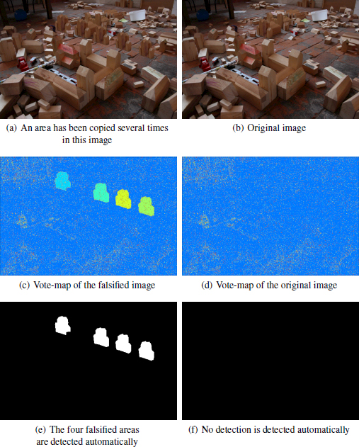
Figure 1.12. In a), an area has been copied four times. The original image is shown in b)
COMMENT ON FIGURE 1.12.– In (c) and (d), the color indicates the origin of the grid of the JPEG blocks detected locally for the falsified and original images, respectively. The navy blue color corresponds to the detected main grid of origin (0, 0). In (c), the areas whose block origin does not match the rest of the image are clearly visible. This detection is made automatic by the a contrario method, whose result can be seen in (e) and (f), where no anomaly is detected in the original image (f), while the falsified image (e) finds the four areas detected as being altered. The original and falsified images come from the database (Christlein et al. 2012).
Likewise, the quantization matrix can be estimated in order to know if it is consistent in each block of the image, and with the global quantization matrix which can be found in the associated header file, which allows the decompression of the image (Thai et al. 2017).
1.6. Internal similarities and manipulations
Finally, we will study the so-called internal manipulations, which modify an image by directly using parts of itself, like inpainting (Arias et al. 2011) and copy and paste.
Unlike other forgeries, these manipulations do not necessarily change residual traces of an image, because the parts used for the modification come from the same image. Therefore, specific methods are necessary for their detection.
The main difficulty in the detection of internal manipulations is the internal similarity of the image. A specialized database was created specifically to measure the rate of false detections between altered and authentic images, but with similar content in different regions (Wen et al. 2016).
The first methods are based on the study of Cozzolino et al. (2015a). Other methods use and compare key points, like those obtained with SIFT (Lowe 2004), which allows similar content to be linked. But this is often too permissive to detect copy and paste. This is why specialized methods, such as proposed by Ehret (2019), propose comparisons between descriptors to avoid the detection of similar objects, which are often distinguishable as shown in Figure 1.13. An example of copy and paste can be found in Figure 1.14.
Neural networks can also be used to detect copy-move manipulations, such as in Wu et al. (2018), where a first branch of the network detects the source and altered regions, while a second branch determines which of the two is the forgery, while other methods generally cannot distinguish the source from falsification.
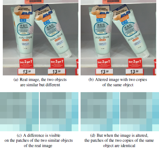
Figure 1.13. The image in a) represents two similar, but different objects, while the image in b) represents two copies of the same object. Both images come from the COVERAGE database (Wen et al. 2016)
COMMENT ON FIGURE 1.13.– The patches in (c) and (d) correspond to the descriptors used by Ehret (2019) associated with the look-at points represented by the red dots for the images that are authentic (a) and falsified (d), respectively. Differences are visible when the objects are only similar, whereas in the case of an internal copy–paste, the descriptors are identical. It is through these differences that internal copy–paste detection methods can distinguish internal copies from the presence of objects that would naturally be similar.

Figure 1.14. Example of detection of copy–paste type modification on the images in Figure 1.13. The original and altered images are in (a) and (d), respectively, the ground-truth masks in (b) and (e), and the connections (Ehret 2019) between the areas detected as too similar in (c) and (f)
1.7. Direct detection of image manipulation
To detect a particular manipulation, one must first be aware of the existence of this type of manipulation. As new manipulation possibilities are continually being created, it is necessary to continually adapt to new types of manipulation, otherwise the detection methods quickly become outdated. To break out of this cycle, several methods seek to detect manipulations without prior knowledge of their nature.
Recently, generative adversarial networks (GAN) have shown their ability to synthesize convincing images. A GAN is made up of two neural networks competing against each other: the first network seeks to create new images that the second one fails to detect, while the second network seeks to differentiate original images from the ones generated by the first network.
Finally, the most common example concerns the use of automatic filters offered by image editing software such as Photoshop. Simple to use and able to produce realistic results, they are widely used. Neural networks can learn to detect the use of these filters or even reverse them (Wang et al. 2019), the training data can be generated automatically, but must deal with the immense variety of filters existing on this software.

Figure 1.15. Structure of the Mayer and Stamm (2019) network to compare the source of two patches. The same first network A is applied to each patch to extract a residue. These residues are then passed on to a network B which will compare their source and decide if the patches come from the same image or not
Recently, Siamese networks have also been used for the detection of falsification (Mayer and Stamm 2019). They are bipartites, as shown in Figure 1.15. They consist of a first convolutional network that is applied independently to two image patches to extract hidden information from each, and then of a second network that compares the information extracted on the two patches to determine whether they come from the same picture. A big advantage of these methods is the ease of obtaining training data, since it is enough to have non-falsified images available and to train the network to detect whether or not the patches were obtained from the same picture. An example of detection with Siamese networks can be found in Figure 1.16.
1.8. Conclusion
In this chapter, we have described methods that analyze an image’s formation pipeline. This analysis takes advantage of alterations made by the camera from the initial raw image to its final form, usually compressed JPEG. We have reviewed the transformations undergone by the raw image, and shown that each operation leaves traces. Those traces can be used to reverse engineer the camera pipeline, reconstructing the history of the image. It can also help detect and localize inconsistencies caused by forgeries, as regions whose pipeline appears locally different than on the rest of the image. With that in mind, it is usually impossible to guarantee that an image is authentic. Indeed, a perfect falsification, which would not leave any traces, is not impossible, although it would require great expertise to directly forge a raw image – or revert the image into a raw-like state – and simulate a new processing chain after the forgery has been done. Falsifiers rarely have the patience nor the skills needed to carry out this task, however one cannot exclude that software to automatically make forged images appear authentic may emerge in the future.

Figure 1.16. Example of modification detection with the Siamese network (Mayer and Stamm 2019)
COMMENT ON FIGURE 1.16.– The forged image comes from the database associated with Huh et al. (2018). The Siamese network gives a similarity score for each patch with a reference patch. The black areas in the Siamese network result correspond to patches that are incompatible with the reference patch.
1.9. References
Agarwal, S. and Farid, H. (2017). Photo forensics from JPEG dimples. In Workshop on Information Forensics and Security. IEEE, Rennes.
Aguerrebere, C., Delon, J., Gousseau, Y., Musé, P. (2013). Study of the digital camera acquisition process and statistical modeling of the sensor raw data. Technical report [Online]. Available at: https://hal.archives-ouvertes.fr/hal-00733538.
Arias, P., Facciolo, G., Caselles, V., Sapiro, G. (2011). A variational framework for exemplar-based image inpainting. International Journal of Computer Vision, 93(3), 319–347.
Bammey, Q., Grompone von Giol, R., Morel, J.-M. (2020). An adaptive neural network for unsupervised mosaic consistency analysis in image forensics. In Conference on Computer Vision and Pattern Recognition (CVPR). IEEE.
Bianchi, T., De Rosa, A., Piva, A. (2011). Improved DCT coefficient analysis for forgery localization in JPEG images. In International Conference on Acoustics, Speech and Signal Processing. IEEE, Prague.
Bracho, R. and Sanderson, A. (1985). Segmentation of images based on intensity gradient information. Proc. IEEE Computer Society Conference on Computer Vision and Pattern Recognition. IEEE Computer Society Press, Amsterdam.
Buades, A., Coll, B., Morel, J.-M., Sbert, C. (2011). Self-similarity driven demosaicking. Image Processing On Line, 1, 51–56.
Chen, Y.-L. and Hsu, C.-T. (2008). Image tampering detection by blocking periodicity analysis in JPEG compressed images. In 10th Workshop on Multimedia Signal Processing. IEEE, Cairns.
Chen, M., Fridrich, J., Goljan, M., Lukáš, J. (2008). Determining image origin and integrity using sensor noise. IEEE Transactions on Information Forensics and Security, 3(1), 74–90.
Choi, C.-H., Choi, J.-H., Lee, H.-K. (2011). CFA pattern identification of digital cameras using intermediate value counting. In Multimedia Workshop on Multimedia and Security. ACM, New York.
Christlein, V., Riess, C., Jordan, J., Riess, C., Angelopoulou, E. (2012). An evaluation of popular copy–move forgery detection approaches. IEEE Transactions on Information Forensics and Security, 7(6), 1841–1854.
Clarke, R.J. (ed.) (1985). Transform coding of images. Astrophysics. Academic Press, London and Orlando, FL.
Colom, M. (2014). Multiscale noise estimation and removal for digital images. PhD Thesis, University of the Balearic Islands, Palma.
Colom, M. and Buades, A. (2013). Analysis and extension of the Ponomarenko et al. method, estimating a noise curve from a single image. Image Processing On Line, 3, 173–197.
Colom, M., Buades, A., Morel, J.-M. (2014). Nonparametric noise estimation method for raw images. Journal of the Optical Society of America A, 31(4), 863–871.
Cozzolino, D. and Verdoliva, L. (2020). Noiseprint: A CNN-based camera model fingerprint. IEEE Transactions on Information Forensics and Security, 15, 144–159.
Cozzolino, D., Poggi, G., Verdoliva, L. (2015a). Efficient dense-field copy–move forgery detection. IEEE Transactions on Information Forensics and Security, 10(11), 2284–2297.
Cozzolino, D., Poggi, G., Verdoliva, L. (2015b). Splicebuster: A new blind image splicing detector. In 2015 IEEE International Workshop on Information Forensics and Security. IEEE, Rome.
Desolneux, A., Moisan, L., Morel, J.-M. (2008). From Gestalt Theory to Image Analysis. Springer, New York.
Donoho, D.L. and Johnstone, I.M. (1994). Ideal spatial adaptation by wavelet shrinkage. Biometrika, 81(3), 425–455.
Donoho, D.L. and Johnstone, I.M. (1995). Adapting to unknown smoothness via wavelet shrinkage. Journal of the American Statistical Association, 90(432), 1200–1224.
Ehret, T. (2019). Robust copy-move forgery detection by false alarms control [Online]. Available at: https://arxiv.org/abs/1906.00649.
Ehret, T. and Facciolo, G. (2019). A study of two CNN demosaicking algorithms. Image Processing On Line, 9, 220–230.
Fan, Z. and de Queiroz, R.L. (2003). Identification of bitmap compression history: Jpeg detection and quantizer estimation. IEEE Transactions on Image Processing, 12(2), 230–235.
Fechner, G. (1860). Elemente der Psychophysik. Breitkopf and Hàrtel, Leipzig.
Fridrich, J., Goljan, M., Du, R. (2001). Steganalysis based on JPEG compatibility. Multimedia Systems and Applications IV, 4518, 275–281.
Getreuer, P. (2011). Zhang-Wu directional LMMSE image demosaicking. Image Processing On Line, 1, 117–126.
Gharbi, M., Chaurasia, G., Paris, S., Durand, F. (2016). Deep joint demosaicking and denoising. ACM Trans. Graph., 35(6), 191:1–191:12.
Ghosh, A., Zhong, Z., Boult, T.E., Singh, M. (2019). Spliceradar: A learned method for blind image forensics. In Conference on Computer Vision and Pattern Recognition Workshops. IEEE, Long Beach.
Gloe, T. (2012). Feature-based forensic camera model identification. In Transactions on Data Hiding and Multimedia Security VIII, Shi, Y.Q. (ed.). Springer, Berlin, Heidelberg.
González Fernández, E., Sandoval Orozco, A., García Villalba, L., Hernandez-Castro, J. (2018). Digital image tamper detection technique based on spectrum analysis of cfa artifacts. Sensors, 18(9), 2804.
Hamilton Jr, J.F. and Adams Jr, J.E. (1997). Adaptive color plan interpolation in single sensor color electronic camera. Document, US Patent, 5,629,734.
Huh, M., Liu, A., Owens, A., Efros, A.A. (2018). Fighting fake news: Image splice detection via learned self-consistency. In European Conference on Computer Vision. ECCV, Munich.
Iakovidou, C., Zampoglou, M., Papadopoulos, S., Kompatsiaris, Y. (2018). Contentaware detection of JPEG grid inconsistencies for intuitive image forensics. Journal of Visual Communication and Image Representation, 54, 155–170.
Immerkær, J. (1996). Fast noise variance estimation. Computer Vision and Image Understanding, 64(2), 300–302.
Kirchner, M. (2010). Efficient estimation of CFA pattern configuration in digital camera images. In Media Forensics and Security Conference. IS&T, San Jose.
Lebrun, M., Colom, M., Morel, J.-M. (2013). Secrets of image denoising cuisine. Image Processing On Line, 2013, 173–197.
Lebrun, M., Colom, M., Morel, J. (2015). Multiscale image blind denoising. IEEE Transactions on Image Processing, 24(10), 3149–3161.
Lee, J.-S. (1981). Refined filtering of image noise using local statistics. Computer Graphics and Image Processing, 15(4), 380–389.
Lee, J.-S. and Hoppel, K. (1989). Noise modeling and estimation of remotely-sensed images. In 12th Canadian Symposium on Remote Sensing Geoscience and Remote Sensing Symposium. IEEE, Vancouver.
Li, W., Yuan, Y., Yu, N. (2009). Passive detection of doctored JPEG image via block artifact grid extraction. Signal Processing, 89(9), 1821–1829.
Lin, W., Tjoa, S., Zhao, H., Ray Liu, K. (2009). Digital image source coder forensics via intrinsic fingerprints. IEEE Transactions on Information Forensics and Security, 4(3), 460–475.
Liu, C., Freeman, W.T., Szeliski, R., Kang, S.B. (2006). Noise estimation from a single image. In Computer Society Conference on Computer Vision and Pattern Recognition. IEEE, Washington DC.
Losson, O. and Dinet, E. (2012). From the sensor to color images. In Digital Color – Acquisition, Perception, Coding and Rendering, Fernandez-Maloigne, C., Robert-Inacio, F., Macaire, L. (eds). ISTE Ltd, London and John Wiley & Sons, New York.
Lowe, D.G. (2004). Distinctive image features from scale-invariant keypoints. International Journal of Computer Vision, 60(2), 91–110.
Mahdian, B. and Saic, S. (2009). Using noise inconsistencies for blind image forensics. Image and Vision Computing, 27(10), 1497–1503.
Mastin, G.A. (1985). Adaptive filters for digital image noise smoothing: An evaluation. Computer Vision, Graphics, and Image Processing, 31(1), 103–121.
Mayer, O. and Stamm, M.C. (2020). Forensic similarity for digital images. IEEE Transactions on Information Forensics and Security, 15, 1331–1346.
Minami, S. and Zakhor, A. (1995). An optimization approach for removing blocking effects in transform coding. IEEE Transactions on Circuits and Systems for Video Technology, 5(2), 74–82.
Nikoukhah, T., Anger, J., Ehret, T., Colom, M., Morel, J., Grompone von Gioi, R. (2019). JPEG grid detection based on the number of DCT zeros and its application to automatic and localized forgery detection. In Conference on Computer Vision and Pattern Recognition Workshops. IEEE, Long Beach.
Nikoukhah, T., Colom, M., Morel, J.-M., Grompone von Gioi, R. (2020). Local JPEG grid detector via blocking artifacts, a forgery detection tool. Image Processing On Line, 10, 24–42.
Olsen, S.I. (1993). Estimation of noise in images: An evaluation. CVGIP: Graphical Models Image Processing, 55(4), 319–323.
Pan, X., Zhang, X., Lyu, S. (2011). Exposing image forgery with blind noise estimation. In Multimedia Workshop on Multimedia and Security. ACM, Buffalo.
Pevny, T. and Fridrich, J. (2008). Detection of double-compression in JPEG images for applications in steganography. IEEE Transactions on Information Forensics and Security, 3(2), 247–258.
Ponomarenko, N.N., Lukin, V.V., Zriakhov, M.S., Kaarna, A., Astola, J. (2007). An automatic approach to lossy compression of aviris images. In International Geoscience and Remote Sensing Symposium. IEEE, Barcelona.
Popescu, A. and Farid, H. (2005). Exposing digital forgeries in color filter array interpolated images. Transactions on Signal Processing, 53(10), 3948–3959.
Rank, K., Lendl, M., Unbehauen, R. (1999). Estimation of image noise variance. IEEE Proceedings – Vision, Image and Signal Processing, 146(2), 80–84.
Shin, H.J., Jeon, J.J., Eom, I.K. (2017). Color filter array pattern identification using variance of color difference image. Journal of Electronic Imaging, 26(4), 1–12.
Thai, T.H., Cogranne, R., Retraint, F., Doan, T. (2017). JPEG quantization step estimation and its applications to digital image forensics. IEEE Transactions on Information Forensics and Security, 12(1), 123–133.
Voorhees, H. and Poggio, T. (1987). Detecting textons and texture boundaries in natural images. In International Conference on Computer Vision. IEEE, London.
Wallace, G.K. (1992). The JPEG still picture compression standard. IEEE Transactions on Consumer Electronics, 38(1), xviii–xxxiv.
Wang, S.-Y., Wang, O., Owens, A., Zhang, R., Efros, A.A. (2019). Detecting photoshopped faces by scripting photoshop. In International Conference on Computer Vision. IEEE, Seoul.
Wen, B., Zhu, Y., Subramanian, R., Ng, T.-T., Shen, X., Winkler, S. (2016). Coverage – A novel database for copy-move forgery detection. In International Conference on Image Processing. IEEE, Phoenix.
Wu, Y., Abd-Almageed, W., Natarajan, P. (2018). Busternet: Detecting copy-move image forgery with source/target localization. In European Conference on Computer Vision. IEEE, Munich.
Yao, H., Wang, S., Zhang, X., Qin, C., Wang, J. (2017). Detecting image splicing based on noise level inconsistency. Multimedia Tools and Applications, 76(10), 12457–12479.
Ye, S., Sun, Q., Chang, E.-C. (2007). Detecting digital image forgeries by measuring inconsistencies of blocking artifact. In International Conference on Multimedia and Expo. IEEE, Beijing.
Zhou, P., Han, X., Morariu, V.I., Davis, L.S. (2018). Learning rich features for image manipulation detection. In Conference on Computer Vision and Pattern Recognition. IEEE, Salk Lake City.
- For a color version of all figures in this chapter, see www.iste.co.uk/puech/multimedia1.zip.
- 1 Available at: www.thispersondoesnotexist.com.
- 2 ENFSI: European Network of Forensic Science Institutes.