8.1.1. The different aims of steganalysis

Many works have been proposed in order to implement different types of steganalysis; we will briefly describe them in the rest of this section:

• – on the one hand, different detection methods can be considered, depending on the Cover media³: images, sounds and videos being different media and compressed differently, they should be treated differently to find hidden information. More broadly, steganography in texts or in computer networks is so different by nature that it seems difficult to analyze them in a similar way;
• – other works, in a way which is more similar to what is done in cryptanalysis, focus on searching for the insertion key from images containing hidden information. These works often require the steganalyst, Eve, to have significant knowledge;
• – in quantitative steganalysis, the aim is to estimate the size of a possible hidden message. We can easily understand that estimating the size of the message can be compared to a binary detection problem. Quite a naive first view involves estimating the size of the hidden message and deciding that the medium is Stego when this estimate exceeds a given threshold;
• – finally, we can mention active steganalysis, in which Eve slightly modifies the transmitted medium in order to preserve its visual appearance while making extraction of the hidden message impossible.

Because of lack of space, it is difficult to tackle all the problems that make up steganalysis in only one chapter. In addition, even though these issues are interesting, we will stick to only the classical framework that concerns the detection of information hidden in digital images.

As we have explained previously, steganalysis was mainly developed to make the evaluation of steganography methods possible. Most works in this field refer to Kerckhoffs’ principle (Kerckhoffs 1883), reworked by Claude E. Shannon, like the fact that “the enemy knows the system used”. In accordance with this principle, steganalysis generally relies on the fact that Eve is only unaware of the inserted message and the insertion key used. We will return to this in greater detail in section 8.3 on the scenario of targeted steganalysis, but this assumes that Eve knows the type of media – generally an image, the insertion algorithm, the size of the message and its statistical properties.

8.1.2. Different methods to carry out steganalysis

The most effective methods for hidden information detection are undoubtedly those based on signatures. In this case, it is possible to detect steganography indirectly, by identifying a particular property that is found systematically when the insertion of a message has been carried out with a certain tool and only in this case. It is therefore a question of detecting a specific feature linked to the use of a precise tool, rather than the presence of hidden information itself. This approach can be compared to what is done for computer security (detection of network attacks or viruses, for example) and is discussed in section 8.2 through some examples.

A second family of more general steganalysis methods, based on modeling and statistical detection, is discussed in section 8.3. In practice, this sort of detection method is very complex to implement, since it requires a very precise statistical model of a Cover image and a Stego image in order to be able to statistically evaluate if a given image is more likely to come from one of these two models. In this section, we precisely define the framework of targeted steganalysis, which is necessary for building statistical models like this.

Section 8.4 deals with the use of statistical learning methods. The most effective steganalysis methods rely on this approach, and so naturally it is those which have been the most widely studied. Here, steganalysis can be subdivided into two distinct problems: the first relates to the extraction of relevant characteristics, and the second relates to learning to automatically classify, based on a vast set of examples, characteristics from Cover and Stego images.

Recently, we have witnessed a spectacular development of deep learning methods, or Deep Learning, which, on the other hand, is carried out in a single phase which combines characterization and classification. The use of these methods for steganalysis is discussed in section 8.5.

This chapter concludes, in section 8.6, with a short, non-exhaustive list of the topics that seem the most interesting and which remain largely open.

8.3.1. Statistical test of χ²

Historically, the first approach that addressed that this problem was proposed in Westfeld and Pfitzmann (1999). Unable to statistically describe what a natural image is, it has been proposed that we model the pixels after using steganography. To explain how this test works, we need to remember how the insertion of a message by least significant bits (LSB) works⁴. In order to insert the ith bit of the message m_i ∈ {0; 1} into the pixel x_m,n, steganography by substitution of the least significant bits modifies the pixel in the following way:

[8.2]

where z_m,n is the pixel of the Stego image and LSB(x_m,n) is the least significant bit of x_m,n.

It is generally accepted in steganalysis that the message inserted, m = (m₁, . . . , m_I), is a sequence of all independent and identically distributed bits (i.i.d) according to a uniform law: [m_i = 0] = [m_i = 1] = 1/2.

The result of the insertion of the bit m_i in the pixel x_m,n is that the Stego pixel can be modeled by the following probability distribution:

[8.3]

with = x + (−1)^x the integer value x whose least significant bit has been inverted.

Furthermore, assuming that all of the pixels are used to hide a (very) large secret message, the distribution of Stego pixels can be modeled as follows:

[8.4]

It then becomes possible to statistically test whether an image is a Stego image by measuring the difference between the theoretical distribution of equation [8.4] and that observed on an analyzed image. This is precisely the purpose of the χ² test that measures the difference between a theoretical distribution and those from observations as follows:

[8.5]

where N_k represents the number of pixels whose value is k and represents the expected number of pixels with the value k.

In fact, equation [8.5] represents a measure of the difference between theoretical distribution and empirical distribution through the term: ². Figure 8.1 illustrates the distribution models of equations [8.4] and [8.5] for a Stego image; in fact, we see a number of pixels k and which are “equalized” on the Stego image.

When the value of χ² is beyond a given threshold, τ, the image is considered to be a Cover image, or statistically too different to the theoretical distribution to be considered a Stego image [8.4]. How should the threshold τ then be set? The authors in Westfeld and Pfitzmann (1999) propose choosing a threshold to make sure that, theoretically, a Stego image is considered as natural with a probability⁵ p₀. For this, the authors use the distribution of χ², which makes it possible to calculate this probability with the following relationship:

[8.6]

with ν = 128 − 1, the “number of degrees of freedom” defined by the number of “pairs of values”, which can be swapped between them.

Figure 8.2 illustrates this way of setting the decision threshold depending on a “false-negative” probability, p₀, set previously. It also allows us to compare the theoretical distribution of the statistic, χ², from equation [8.5] with the theoretical distribution of χ². The difference between the observations and the theoretical model is mainly due to the fact that the vast majority of the images do not have pixels with all the values between 0 and 255, and therefore have a number of degrees of freedom less than ν = 128 − 1.

The strength of the χ² test is that it offers a statistical test without having to solve the (very tricky) problem of modeling the statistical distribution of pixels of a Cover image. In fact, the test essentially proposes checking whether the pixels of an analyzed image correspond to the model of a Stego image; otherwise the image is considered to be a Cover image by default. Another use of this test is to try to set the detection threshold, τ, based on a missed detection probability, p_χ² (τ), defined in equation [8.6].

Unfortunately, this test is not very efficient, especially since it does not model the statistical distribution of a Cover image, but only the Stego image. In statistical detection, when only one of the two hypotheses can be characterized, we generally carry out a “goodness-of-fit” test, measuring the adequacy of the observations to this model, and this is generally less reliable than when you can exactly characterize the two competing hypotheses, as proposed by the likelihood-ratio test presented in section 8.3.2.

8.3.2. Likelihood-ratio test

In order to fully understand the approach presented in this section, it is necessary to formalize steganalysis and statistical detection.

A statistical test is a function δ, which, from a group of observations, X, returns a binary decision: δ : X → {0, 1}, so that the hypothesis, ₀, is accepted if δ(X) = 0. Let us briefly recall that a test is never perfect and that there are two possible types of errors: false-positive and false-negative (or false alarm and no detection). In general, the hypothesis ₀ is said to be “null”, and corresponds to a “normal” case, while the alternative hypothesis, ₁, corresponds to the difficult situation that we want to detect. The false-positive, therefore, corresponds to the case where the test decides to accept the hypothesis ₁ when, in reality, the observations come from the hypothesis ₀.

In the case that we are interested in, the analyzed image is a Cover image which is classified as a Stego image. On the other hand, a false-negative corresponds to the case where the test accepts the hypothesis ₀, when the observations really come from the alternative hypothesis ₁; for steganalysis, this is the case where the guardian, Eve, misses the detection of a Stego image.

In order to show how weak the χ² test is, we need a statistical model of the Cover images. This is built by assuming that the pixels are statistically independent and all come from a Gausian distribution:

[8.7]

where µ_m,n represents the mathematical expectation of the pixel (i.e. its “average” or theoretical value), and represents the noise variance.

This is a model commonly used in image processing, which assumes that an image can be decomposed into a theoretical “content” and noise, linked to the camera defects. To be more precise, the pixels are represented by integer values and, for the sake of simplicity, we assume that this has no impact on the probability distribution of the pixels:

[8.8]

First, we study the case where Alice uses steganography by LSB substitution⁶. Each pixel can be modified with the same probability of , which relates to the ratio of the number of bits of the inserted message (I), per pixel (MN), and the distribution of a Stego pixel then becomes:

[8.9]

Truth	Hypothesis 0: (Cover image)	Hypothesis 1: (Stego image)
Result
Accept Hypothesis 0	Correct decision	False-negative (missed detection) (pFN: 1 − ς)
Accept Hypothesis 1	False-positive (false alarm) (pFP: α= [δ(X)=1|0])	Correct decision (ς= [δ(X)=1|1])

How can we use these statistical models to decide whether an examined image, X, comes from the hypothesis model instead ₀⁷, or from the hypothesis ₁⁸?

There are several solutions that have one central element in common, the likelihood ratio (LR), which is expressed as:

[8.10]

with p₀ and p₁, which are the statistical distribution models for Cover and Stego images, respectively, defined by equations [8.8] and [8.9], respectively.

The second part of the equality of equation [8.10] results directly from the statistical independence model between the pixels which, although not totally exact, is very widely used because it significantly simplifies things.

Clearly, the likelihood ratio (LR) is greater if the probability of observing the data to be analyzed is greater under ₁ than under ₀; conversely, if the probability of observing these data is much greater under ₀ than under ₁, the LR will be low. Based on this observation, the likelihood ratio test simply involves thresholding this likelihood ratio: δ(X) = ₀ if Λ(X) < τ and δ(X) = ₁ and Λ(X) ≥ τ.

The use of the LR test is theoretically justified because the Neyman–Pearson lemma states that it helps achieve the greatest power⁹ ς for a false-positive probability, α, set at α = [Λ(X) > τ]. This last relationship also makes it possible to set the threshold in order to respect a previously established false-positive rate.

Using the Cover image model of equation [8.8] and the Stego image model of equation [8.9], the LR is written as:

[8.11]

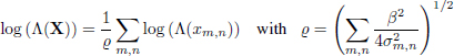
For the sake of simplicity, the logarithm of LR is generally used. This is to replace the product in equation [8.11] by the sum. Moreover, by using the definition of p₀(x_m,n) equation [8.8], a (slightly tedious) calculation makes it possible to simplify the previous relationship as follows (Cogranne 2011):

[8.12]

In this approach, the most interesting thing is not so much having a simple relationship, making the calculation of the likelihood ratio possible (although some simplifications had to be made), but more being able to characterize the statistical distribution of the latter and therefore, in fine, controlling the probabilities of false alarms and non-detection.

In particular, it is possible to show the mathematical expectation and variance of the term log (Λ(X)) for a Cover image given by:

[8.13]

It is then possible to standardize the LR as follows:

[8.14]

so that, in accordance with the central limit theorem (Lehmann and Romano 2005, theorem 11.2.5), it is possible to calculate the statistical distribution of the LR-log for a given image:

[8.15]

With the Gaussian distribution being fairly easy to use, we can easily calculate the decision threshold, τ, to ensure a fixed false-positive probability, α₀: τ(α₀) = Φ⁻¹ (1 − α₀) so that [log (Λ(X)) > τ (α₀)|₀] = α₀. Similarly, the power of the test ς can be calculated as the probability, [log (Λ(X)) > τ |₀] = 1 − Φ (τ − ϱ).

Many observations are necessary to understand these different results. On the one hand, let us note that it is very “typical” for the mathematical expectation of the LR for a Stego image to be equal to its variance. It is for this reason that the normalization factor, ϱ, in equation [8.14] also corresponds to the expectation in equation [8.15].

We also note that all the previous calculations require knowledge of the mathematical expectation, µ_m,n, and the variance, , of each of the pixels, but, in practice, these variables are not known. It is therefore suggested that we replace them with estimates, which are quite hard to obtain “accurately”, and this is where the application of this approach becomes much more complicated and the guarantee of the error probabilities in particular becomes very difficult. Some results are presented in Figure 8.3, using the ALASKA image database (Cogranne et al. 2019). Figure 8.3(a) shows that the distribution of the LR-log obtained for Cover images is fairly consistent with the theory. For Stego images, it depends on the ϱ factor, which varies for each image, creating this “spread”. Figure 8.3(b) compares the false-positive probability depending on the decision threshold, τ, in theory and in practice, using two different image bases. We can also see that this property is valid for “fairly high” probabilities. However, note that, in the case where we want to obtain very low false-positive rates, the estimates are not precise enough to offer relevant guarantees. Finally, Figure 8.3(c) shows the performances obtained through a ROC (Receiver Operating Characteristic) curve, which presents a false-positive probability, α₀(τ), depending on the detection power ς(τ). We can see that for an insertion rate β ≈ 0.09 (24 kilobits inserted into images of 512 × 512 pixels), the performance is very good on the two bases used for high error probabilities.

8.3.3. LSB match detection

Essentially, the detectors presented in section 8.3.2 show that steganography by substitution of the LSB clearly introduces a bias by increasing even values and decreasing odd values. This explains why this insertion method is to be avoided, to benefit the correspondence (LSBM or LSB±1), which modifies the least significant bits, according to the insertion rule defined in section 5.3.1.

After having presented the application of a statistical test for steganalysis in detail, we can address the detection of LSB±1, which has been studied in the literature through “simple” tests much less. We will also consider the case of an adaptive steganography scheme, that is, the probability of using the pixel x_m,n is potentially different for each pixel¹⁰ and will therefore be denoted β_m,n. The reader will note that it is very easy to replace the “average insertion rate”, β with an insertion rate for each pixel, β_m,n, without any additional modification, in equations [8.9] and [8.11]–[8.14].

We will not explain all the details of the calculations, which can be found in Cogranne (2011) and Sedighi et al. (2016a), but the LR-log calculation for the least significant bits correspondence leads, after a few simplifications, to:

[8.16]

Again, the most interesting thing here is calculating the error probabilities of this test and, using the central limit theorem like before, this requires knowing the first two moments, which are given by:

[8.17]

The comparison between the LR for LSB substitution detection, given in equation [8.12], and the LR for the detection of LSB±1, given in equation [8.16], shows that the detection of LSBR (substitution) is essentially based on a deviation from the expectation through the term (x_m,nµ_m,n). Conversely, the detection of LSB±1 is essentially based on a difference between the theoretical variance and that observed through the term (x_m,n − µ_m,n)². However, if estimating the mathematical expectation of pixels is widely studied¹¹, the precise estimate of the variance of pixels is much harder and has been studied much less. We also want to detect a deviation from a variance that is not known and needs to be estimated, regardless of the presence of hidden information. All of this explains why the statistical steganalysis methods tackling adaptive insertion methods are not as efficient as the LSB substitution steganalysis seen in section 8.3.2.

The application of statistical detection explains why the steganalysis of LSB±1 is more difficult; it should be noted that the performance study also shows that, for a given pixel, the “detectablility” essentially depends on the “insertion-on-noise relationship”, defined by in the relationships of equation [8.17].

An interesting application of the theory of hypothesis testing has been to use this result concerning the “statistical detectability” of each pixel to design an insertion algorithm (Sedighi et al. 2016a) which, instead of minimizing the heuristic distortion, minimizes the theoretical detectability. Although this requires estimating the mathematical expectation and the variance of each pixel (which remains an unresolved problem), it has shown its effectiveness. More details on this application of the theory of hypothesis testing in steganography are given in section 5.3.2.2.

To conclude this section on statistical steganalysis, let us mention that a method of statistical steganalysis on JPEG images has recently been proposed that amazes with how efficient it is. This method, presented by Butora and Fridrich (2020) and Cogranne (2020), exploits the fact that the pixels are quantized before using the discrete cosine transform (DCT). For a compressed image, it is possible to decompress it¹² and to measure the variance of the quantization noise by:

[8.18]

where M and N are the number of lines and columns of image X, and round (·) is the rounding function to the closest integer value.

If information has been hidden in the DCT coefficients, the rounding error in the spatial domain makes it possible to obtain the statistic defined in equation [8.18], which will tend to increase. This test is really effective (it was slightly improved in Cogranne et al. (2020b) with a “near-perfect” detection of a few hundred bits). This can be explained by the fact that it is based on a very precise model and does not depend on the parameters to be estimated, but only on the quantization noise which is the same regardless of the image analyzed. However, this is a very specific case that can be equivalent to incompatible signature detection (see section 8.2).

8.4.1. Extraction of characteristics in the spatial domain

8.4.1.1. SPAM characteristics

It would obviously take too long to describe the evolution of steganalysis up to modern techniques in detail, but note that, generally, a keystone of current methods originated in Pevný et al. (2010), which uses the differences between adjacent pixels that we will denote D^→:

[8.19]

with →, which here represents the horizontal direction in which the differences are calculated, among the eight possible used .

On the basis of these differences, it is suggested that we estimate the frequency with which successive differences are found in an image. Representing an empirical frequency corresponds to a count that is generally, simply yet inaccurately, known as “histogram” in steganalysis. These counts are arranged in vector:

[8.20]

with [·], the indicator function, [e] = 1 if the event e is true – and [c] = 0 otherwise – and T, the maximum difference threshold considered.

Given that the values of adjacent differences together on neighboring positions are counted, these vectors are called “co-occurrence” in steganalysis. This concept can be generalized by using more than two disjoint values at the cost of increasing the number of possible co-occurrence values. In fact, by using co-occurrences of c adjacent differences between T and T, it gives (2T +1)^c different values of possible co-occurrences. Finally, the last step proposed in Pevný et al. (2010) aims to limit the number of characteristics by gathering together the values calculated for opposite directions, for example ← and →, or even ↖ and ↘. The authors propose grouping together “diagonal” directions and horizontal and vertical directions:

[8.21]

This step, called “symmetrization”, aims to reduce the number of characteristics.

The original SPAM, Subtractive Pixel Adjacency Matrix (Pevný et al. 2010) characteristics, use triplets of three adjacent differences, c = 3, f_k,l,m (kown as second order), and three distinct values for each T = 3. This means counting a distinct number of “co-occurrences” of (3 × 2 + 1)³ = 7³ = 343. Adding the fact that diagonal co-occurrences are distinguished from horizontal and vertical co-occurrences during the symmetrization phase, this gives a total of 686 characteristics.

Clearly this is quite a high number of characteristics (also know as dimensions) compared to the problems generally studied in the field of statistical learning.

8.4.1.2. RM characteristics

However, it has been empirically observed that, for the particular case of steganalysis, which essentially involves a very weak signal detection within the Cover media, generalizing an approach like this makes it possible to improve the detection performance. The approach that we have briefly described was largely developed afterward in a methodology whose operating principle is illustrated in Figure 8.5. This figure illustrates the “Spatial Rich Model” operating as proposed in Fridrich and Kodovsk (2012). This is essentially an improvement of the method proposed in Pevný et al. (2010). Furthermore, these models are fairly standard, and also illustrate the fact that the current methods of steganalysis are divided into four main stages, which are (1) calculation of residuals; (2) quantization and thresholding; (3) counting co-occurrences and finally (4) redundancy reduction by symmetrization.

Calculating residuals is generally done by using a linear filter. From an image, X, whose pixels are given by x_m,n, we apply the same relationship between adjacent pixels on the whole image:

[8.22]

This weighted sum of neighboring pixels is a convolution operation, R⁽ⁿ⁾ = X * K(n), whose kernel K⁽ⁿ⁾ specifies the value of these weighting factors. We generally speak of a low-pass filter when ∑_i,j k_i,j = 1; it is typically a “smoothing”, aiming to decrease the “noise”. On the other hand, in steganalysis, the term “residuals” is used to characterize high-pass filtering, characterized by ∑_i,j k_i,j = 0, k_0,0 = –1. In other words, it is about “estimating” the value of a pixel, x_m,n, from its neighbors, , and then calculating the difference, , which corresponds to the “estimation error”, due to the filter, K⁽ⁿ⁾.

To be able to catch all the possible traces due to steganography, the number of filters is important; 78 residuals are used to construct the RM characteristics presented in Fridrich and Kodovsk (2012).

The second step is quantization and thresholding. Generally, weighting factors used in the kernels K⁽ⁿ⁾ are not integers, and the residuals R⁽ⁿ⁾ must be grouped together into “close” values to be able to work out “histograms”. The general idea is dividing the residuals, R⁽ⁿ⁾, by a quantization step, q, and then rounding the results. The quantization step, q, then determines the “granularity” of the histogram. A very large step gives a rough histogram: for example, a step of q = 10 leads to rounding to the nearest 10; on the other hand, a step of q = 1 leads to rounding to the nearest integer. Thresholding simply involves limiting the range of possible values (despite quantization) in order to limit the extent of resulting “co-occurrences”. It is simply suggested that we only count the values of the residuals below a certain threshold, T, and ignore the values beyond.

Finally, this second step can be represented by:

[8.23]

with Threshold_T, the thresholding operation with the threshold T, and Round, the rounding operation to the nearest integer.

In Spatial Rich Models (Fridrich and Kodovsk 2012), three distinct quantization steps are used, (q = {1, 2, 3}), but the threshold is always set at T = 3, in order to be able to represent smaller or greater residue values, depending on the quantization step.

The third step aims to represent the “residuals” through histograms with several dimensions or co-occurrences. This mainly allows a better representation of the global statistical properties of the residuals, regardless of their positions in an image, but also to reduce the amount of data and, finally, to have an identical representation, whatever the size of the image analyzed. The co-occurrence calculation for a given type of residual, R⁽ⁿ⁾, is done, as explained in equation [8.20], by counting the number of adjacent values, whose values are all equal to a certain pattern. It is therefore a generalization of equation [8.20] to a tuplet of c adjacent residuals. It is also worth noting that by using c adjacent residuals, we can also multiply the directions, which can be much more general than just the eight directions considered, in the case of pairs. The calculation of co-occurrences is generally limited to vertical and horizontal directions, since all possible paths would become too large with co-occurrences of dimension c = 4, like the ones used in Fridrich and Kodovsk (2012).

Finally, the last step involves merging, similar co-occurrences, typically vertical to the left or to the right, generally by calculating an average. The underlying principle is that there is no objective reason to assume that traces of steganography are represented differently in one direction than they are in another. Symmetrization is a harder step to generally define, since it greatly depends on the filters used to calculate the residuals, on the one, and the co-occurrences used, on the other. Generally, we agglomerate the different directions (vertical and horizontal co-occurrences), as well as the filters that can be deduced from one another by symmetry. This stage makes it possible to greatly reduce the number of characteristics used. In fact, consider the classic case of characteristics from rich spatial models (Fridrich and Kodovsk 2012). We count 78 distinct filters with three quantification steps, a thresholding with the threshold T = 2, and co-occurrences calculated horizontally and vertically. Eventually, an image characterized by RMs has (after symmetrization) 34,761 features.

8.4.2. Learning how to detect with features

Once the features have been extracted, a classification phase remains to be implemented. More precisely, it is necessary to extract these features for a large amount of Cover images in order to then hide information in these images using a steganography method to generate Stego images, and finally to extract characteristics from these Stego images. Learning a classification rule in such a framework is part of supervised statistical learning: we have seen two feature sets, the first for images without Cover information and the second for Stego images. There are many supervised statistical learning methods; in general, this corresponds mathematically to an optimization problem to find the parameters of a function, making it possible to maximize the detection performance. Since in steganalysis the main adapted classifiers are linear, we will focus on this type of method.

Consider two bases of L features calculated on I images, that we denote in matrix form C = (c⁽¹⁾, . . . , c^(I)) for Cover images (of class – 1) and S = (s⁽¹⁾, . . . , s^(I)) for Stego images (of class 1). A linear classifier is based on a projection of the features on a discrimination vector, . This operation is a weighted sum of features. The goal is therefore to find a vector of the weighting coefficients, w, which makes it possible to differentiate the Cover and Stego data after projection. A simple criterion for this involves seeking weighting coefficients, w, so that the vectors c_i are close to the value −1, while the vectors s_i are close the value 1.

If large vectors, y₀ and y₁, are created, with the first vector containing I times the value of −1 and the second vector containing I times the value of 1, it is then a question of finding the weighting factors, w, that minimize the difference between the values w^T C and y₀ (and vice versa between w^T × S and y₁), let + .

This method actually comes to a minimization problem, in the sense of least squares. This approach is particularly interesting, since an analytical solution is given by:

[8.24]

where X is a matrix that groups together features X = (C, S) and, similarly, the vector y contains all label values y = (y₀; y₁).

Therefore, this method functions correctly, and it is generally useful to add a regularization factor, which makes it possible to find a compromise between a “simple” solution and a solution that is adapted to the data used for learning. It is this method which was proposed in Cogranne et al. (2015), and which allows performance that is very close to the state of the art in just a few seconds (for 10,000 images and 40,000 characteristics).

An interesting alternative approach that is based on another linear classifier is the Fisher approach, which is very similar to the previous one, but aims to maximize the separability criterion:

[8.25]

where µ_i is the mean of the features for the images of the class i, and Σ_i is the covariance matrix of the features of the class i.

This method also presents the advantage of having a directly calculable solution:

[8.26]

The main attraction of the method proposed in Kodovsk et al. (2012) is the use of a variety of classifiers. For this, many classifiers are trained on “sub-sets” of images and/or on “sub-sets” of characteristics. The attraction is mainly based on the fact that this specific training and this procedure for multiplying classifiers makes it possible to eventually build a “robust”, nonlinear and efficient classifier. This method has been improved in Cogranne and Fridrich (2015), but, in both cases, the results are slightly better than those obtained with a simple linear classifier for a much greater computational complexity (of the order of 20–100 times more).

8.5.1. Foundation of a deep neural network

In the following sections, we recall major concepts of a CNN; we will recall the basic building blocks of a network based on the Yedroudj-Net network, which was published in 2018 (Yedroudj et al. 2018b) and which uses ideas that are present in Alex-Net (Krizhevsky et al. 2012), as well as those present in networks developed for steganalysis, including the very first network by Qian et al., the Xu-Net network (Xu et al. 2016) and the Ye-Net network (Ye et al. 2017).

8.5.2. The preprocessing module

In Figure 8.6, we can see that, in the preprocessing module, the image is filtered by 30 high-pass filters. The use of one or many high-pass filters as preprocessing is present in the majority of networks used for steganalysis during the period between 2015 and 2019. As an example, the kernel “square S5a” (Fridrich and Kodovsk 2012) is given by:

[8.27]

This initial filtering step allows the network to converge faster and is probably necessary for good performance when the training base is too small (Yedroudj et al. 2018a) (only 4,000 Cover/Stego pairs of pixel size 256 × 256). The filtered images are then transmitted to the first convolution block of the network. The Yedroudj-Net network has five convolution blocks (Yedroudj et al. 2018b), like the Qian et al. network (Qian et al. 2015) and the Xu et al. network (Xu et al. 2016).

Note that the recent SRNet network (Boroumand et al. 2019) does not use fixed pre-filters, but learns the values of filters. This requires a much larger database (more than 15,000 Cover/Stego pairs of 256 × 256 pixels), and possibly using a preliminary training to start from a good initialization. There is also a debate in the community as to whether we should use fixed filter values, initialize the filter values with preselected values and then refine these values by training or have a random initialization and leave the network to learn the values of the filters. At the time of writing this chapter, we think that the best choice is related to the architecture of the network, the size of the training database used and the possibility of using pre-training/transfer learning.

8.6.1. The problem of Cover-Source mismatch

The first problem that we will describe is Cover-Source mismatch (CSM); this problem is actually a fairly general case in the field of statistical learning, where it is referred to as “generalization”. In practice, this is the mismatch between the learning base, on which the classifier is trained, and the test base on which we want to detect the presence of hidden information. The defining feature of steganalysis is double, compared to CSM. On the one hand, in steganalysis we want to detect very weak signals; on the other hand, we generally work with characteristics of (very) large dimensions. Together, these two features mean that the detection methods will be very sensitive to the learning bases and difficult to generalize.

A fairly exhaustive study concerning the evaluation of the factors leading to CSM was carried out in Giboulot et al. (2020), showing, for example, the major role of image processing. Unfortunately, there is no work to understand the root causes yet, and, as a result, it remains very difficult to overcome this problem.

8.6.2. The problem with steganalysis in real life

Similarly, steganalysis in real life been not been explored much (Ker and Pevný 2014). In fact, as we mentioned in the introduction, steganalysis was developed with the main aim of evaluating the different methods of steganography. To do this, the community generally works using the targeted steganalysis scenario and with specific image databases, in particular the BOSS (Bas et al. 2011) database consisting of images from seven reflex cameras (no smartphone or compact), all processed the same, starting from the RAW file. Work has shown that developing these RAW images in different ways can lead to very different results (Sedighi et al. 2016b). A first competition was launched for this purpose with a much more heterogeneous image base (Cogranne et al. 2019) and proposals show the difficulty of carrying out steganalysis on heterogeneous images. The winners, in particular, relied on a increase of learning, according to the JPEG compression parameters (Yousfi et al. 2019), but many questions about steganalysis in real-life remain open.

8.6.3. Reliable steganalysis

A problem that is fairly similar to the previous two concerns reliable steganalysis. In fact, as we mentioned in section 8.3.2, a test is inevitably full of errors (false-positives and false-negatives), and the result depends greatly on the application context. In steganalysis, it is important to minimize false-positives, given the large number of images that we may have to analyze. On the other hand, methods based on statistical learning generally aim to minimize the overall error rate, P_E. However, assuming that it is possible to design a detection method where the probabilities of false-positive and false-negative are both about 1%, it is clearly unrealistic to use this method in practice. It is clear to argue that, with a Bayesian approach, an image considered as being steganographed by a detector like this would actually be more likely from a false-positive, given that on an image-sharing site such as Flickr, probably less than 1% of images actually contain hidden information.

Therefore, the crucial question arises of how to design a reliable steganalysis method that would guarantee a very low probability of false-positive; typically, a probability of false-positive less than 10⁻⁶ (i.e. less than 1 in 1 million). We have seen that the theory of hypothesis tests makes it possible to design methods of steganalysis like this, but relies on a statistical model of the images which is not necessarily exact, even more so when certain parameters have to be estimated. A very interesting study in Pevný and Ker (2015) studies the possibility of learning with the criterion of minimizing the probability of false-positive, if the power ς is fixed at 50%. However, this preliminary work deserves to be looked at in more depth, and steganalysis methods providing a precise “p-value”²⁰ are sorely lacking.

8.6.4. Steganalysis of color images

As indicated in Chapter 4, the vast majority of images today are in color; for practical applications, it is therefore necessary to study this type of image. However, academic work differs from practical use since the vast majority of work in steganalysis relates to “grayscale” images (see Cogranne et al. 2019, 2020a, 2020b).

On the contrary, detection of hidden information in color images seems more interesting in practice. This subject remains largely undiscovered. In fact, a significant number of researchers think that a color image can be represented by three images in grayscale (one red, one green and one blue), which can be analyzed separately.

However, it seems intuitive to consider that the color channels are statistically correlated, in particular due to the “demosaicing” during the acquisition and processing of images. However, work which has been carried out in this field has not shown a great improvement by analyzing the components together (Goljan et al. 2014; Abdulrahman et al. 2016). For example, the first work in this field (Goljan et al. 2014) proposed adding histograms obtained from pixel values in different colors. This certainly allowed a slight improvement in detection, but below what was expected.

Finally, this field of study has not been studied very much for color images compressed with the JPEG standard. This is more harmful, because JPEG color images do not represent green, red and blue, but luminance/chrominance components whose statistical correlations are less significant. On the other hand, color channels are treated separately in the JPEG standard, so they should be analyzed in different ways. Unfortunately, detection of steganography in JPEG color channels has hardly ever been studied (see, for example, (Taburet et al. 2018) and the articles (Cogranne et al. 2019; Yousfi et al. 2019) relating to the ALASKA steganalysis challenge and about JPEG color images).

8.6.5. Taking into account the adaptivity of steganography

A very different problem, already mentioned in section 8.5.2.3 in the context of neural networks, is about the consideration of the “selection channel” for steganalysis. The channel selection shows the probabilities of using each pixel, β_m,n. Clearly, it seems interesting (as shown by equations [8.14] and [8.16]) that a detector can use a, possibly misleading, estimate of these probabilities of use. But this is not very effective with current detection methods. For example, one of the first advances proposed in the field (Denemark et al. 2014) involves replacing the calculation of co-occurrence histograms (see section 8.4.1) by adding, for each of the blocks considered, the maximum probability of modification, β_m,n, of this sample. In this study (Denemark et al. 2014), the authors indicate that they have tried several weighting functions and finally found that the maximum obtains the best results, in terms of performance. In addition, the authors indicate that this function is also robust to a misestimation of the selection channel, β_m,n. This is particularly important, since this quantity is not directly attainable and therefore must be estimated. This requires knowing the insertion method and size of the message and, in practice, the performances obtained from the estimated probability or from the real probability are very similar. In all cases, SCA methods (SCA) remain very ad hoc, and they are empirically explained, mainly by results in terms of statistical detection performance.

8.6.6. Grouped steganalysis (batch steganalysis)

A problem that has also been studied very little concerns “grouped” steganography, also called “batch” steganography (Ker and Pevný 2012). This is a more general scenario where Alice can “spread out” her message in many different images, which are then sent to Bob. The steganalyst, Eve, must therefore observe a batch of images, q, and make a “grouped” decision about all of these images: they may all be Cover images, or some may contain a variable part of the message to hide. For steganography²¹, this case can be modeled as a problem of message allocation, which must be dispersed in several images in order to minimize the probability of detection. For the steganalyst, Eve, the job of analyzing a batch of images is much more tricky. Many questions remain open, in particular: How can you analyze a lot of images, unknown at first? Is it better to use a method designed to analyze several images together, or should you carry out q independent image analyzes? Finally, should not the order of the images be taken into account? Some works have been proposed, in particular (Cogranne et al. 2017; Pevný and Nikolaev 2015), which are based on a detector adapted to the analysis of each image individually. The first article studies how to regulate the “(continuous) scores” obtained for each image. The second work (Pevný and Nikolaev 2015) carries out a detection in two stages: a histogram of the same “scores” is first constructed, then a second classifier is trained to identify the batches of Cover images. More recently, a study relating to the lack of knowledge of the strategy of spreading the message has been proposed in Zakaria et al. (2019).

8.6.7. Universal steganalysis

The last issue that we want to tackle is universal steganalysis. Again, this is a more general framework than targeted binary decision, which, as we have shown, makes it possible to assess a specific method of steganography. In practice, it is interesting to design steganalysis methods that work when neither the size of the message nor the insertion algorithm are known. Steganalysis without knowing the size of the message refers to so-called “quantitative” approaches, that is, aiming to estimate the size of the inserted message (Pevný et al. 2009). The study of the performance of the general classifier (Cogranne and Fridrich 2015), in the context where the size of the message is unknown, specifically shows that the latter (Kodovsk et al. 2012) cannot be used directly, since the detection threshold is fixed according to the steganographed images used during training. The approach proposed in Pevný et al. (2009) essentially involves using images containing different sized messages during training.

Similarly, multi-class steganalysis has not received much attention. Again, the extension of the general classifier has been considered with this in mind (Cogranne and Fridrich 2015) by using two simple and relatively efficient approaches; the first, known as “Cover media versus the rest”, involves creating an alternative hypothesis gathering all the possible insertion algorithms and, in the end, carrying out a statistical learning aimed at detecting any of the steganography methods. On the other hand, the second approach involves considering H + 1 hypotheses, relating to the H insertion algorithms considered, then the case of Cover images is added. To detect steganography and identify the insertion method, it is possible to create many classifiers that are specifically trained to distinguish between two hypotheses. Analyzing an image therefore requires using all the classifiers to then choose the hypothesis that gathers the most “votes” from the set of all the classifiers.