To understand how the backpropagation method works, let's look at an example.

We'll introduce the following indexing for all expression elements: is the index of the layer, is the index of the neuron in the layer, and  is the index of the current element or connection (for example, weight). We use these indexes as follows:

This expression should be read as the element of the neuron in the layer.

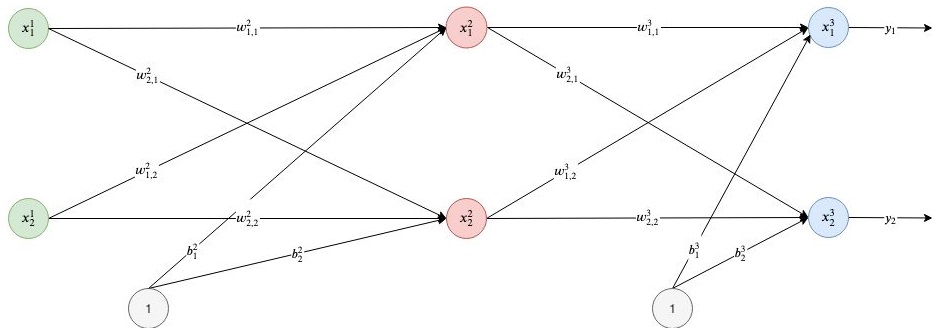
Let's say we have a network that consists of three layers, each of which contains two neurons:

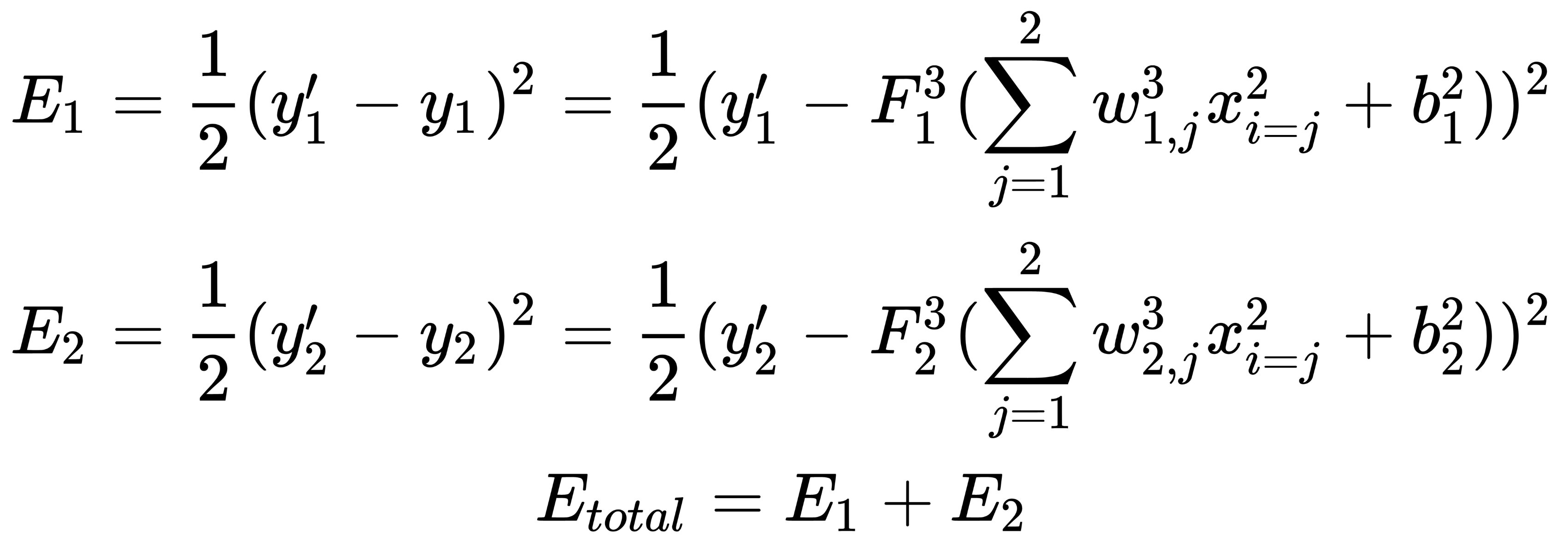
As the loss function, we choose the square of the difference between the actual and target values:

Here,  is the target value of the network output, is the actual result of the output layer of the network, and  is the number of neurons in the output layer.

This formula calculates the output sum of the neuron, , in the layer, :

Here,  is the number of inputs of a specific neuron and  is the bias value for a specific neuron.

For example, for the first neuron from the second layer, it is equal to the following:

Don't forget that no weights for the first layer exist because this layer only represents the input values.

The activation function that determines the output of a neuron should be a sigmoid, as follows:

Its properties, as well as other activation functions, will be discussed later in this chapter. Accordingly, the output of the i ^th neuron in the l ^th layer () is equal to the following:

Now, we implement stochastic gradient descent; that is, we correct the weights after each training example and move in a multidimensional space of weights. To get to the minimum of the error, we need to move in the direction opposite to the gradient. We have to add error correction to each weight, , based on the corresponding output. The following formula shows how we calculate the error correction value, , with respect to the  output:

Now that we have the formula for the error correction value, we can write a formula for the weight update:

Here,-  is a learning rate value.

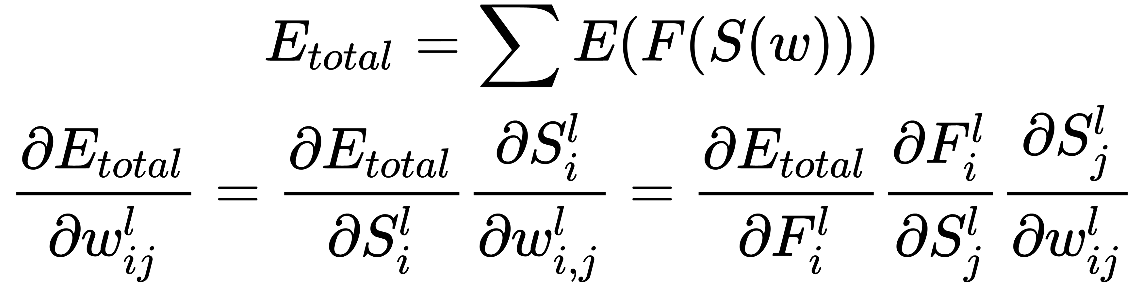
The partial derivative of the error with respect to the weights, , is calculated using the chain rule, which is applied twice. Note that  only affects the error only in the sum, :

We start with the output layer and derive an expression that's used to calculate the correction for the weight, . To do this, we must sequentially calculate the components. Consider how the error is calculated for our network:

Here, we can see that does not depend on the weight of . Its partial derivative with respect to this variable is equal to :

Then, the general expression changes to follow the next formula:

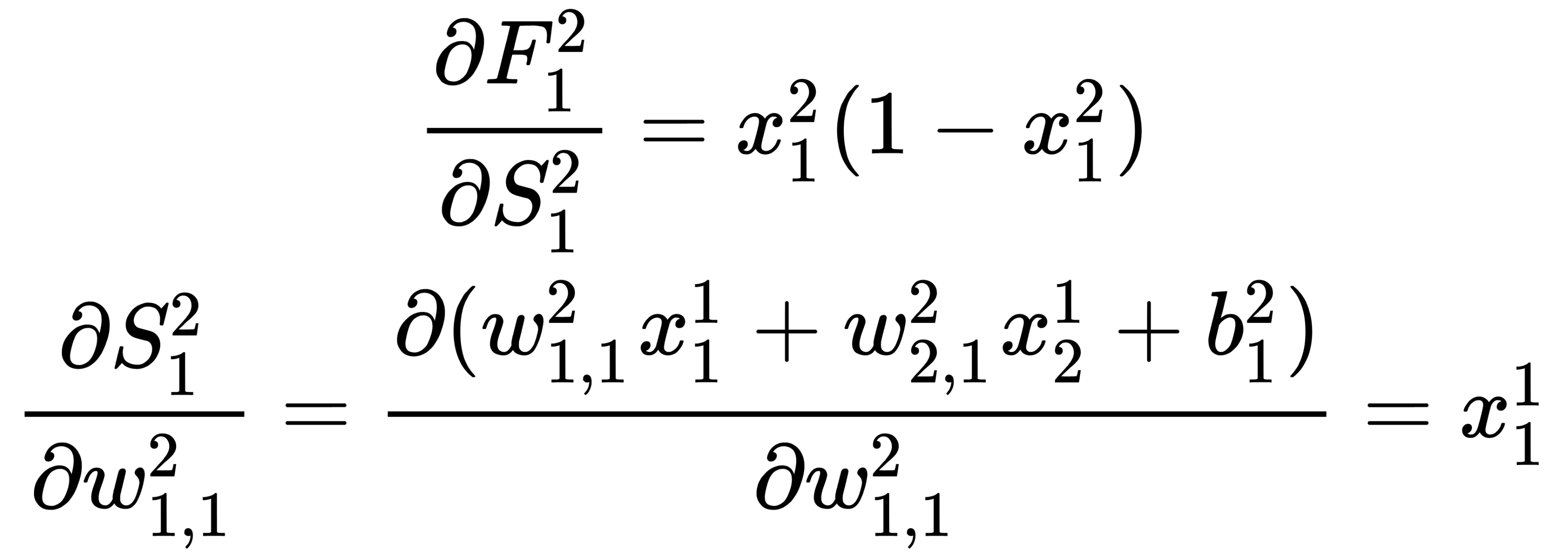
The first part of the expression is calculated as follows:

The sigmoid derivative is , respectively. For the second part of the expression, we get the following:

The third part is the partial derivative of the sum, which is calculated as follows:

Now, we can combine everything into one formula:

We can also derive a general formula in order to calculate the error correction for all the weights of the output layer:

Here,  is the index of the output layer of the network.

Now, we can consider how the corresponding calculations are carried out for the inner (hidden) layers of the network. Let's take, for example, the weight, . Here, the approach is the same, but with one significant difference – the output of the neuron of the hidden layer is passed to the input of all (or several) the neurons of the output layer, and this must be taken into account:

Here, we can see that and have already been calculated in the previous step and that we can use their values to perform calculations:

By combining the obtained results, we receive the following output:

Similarly, we can calculate the second component of the sum using the values that were calculated in the previous steps –  and :

The remaining parts of the expression for weight correction, _, are obtained as follows, similar to how the expressions were obtained for the weights of the output layer:

By combining the obtained results, we obtain a general formula that we can use to calculate the magnitude of the adjustment of the weights of the hidden layers:

Here,  is the index of the hidden layer and is the number of neurons in
the layer, .

Now, we have all the necessary formulas to describe the main steps of the error backpropagation algorithm:

1. Initialize all weights, , with small random values (the initialization process will be discussed later).
2. Repeat this several times, sequentially, for all the training samples, or a mini-batch of samples:

1. Pass a training sample (or a mini-batch of samples) to the network input and calculate and remember all the outputs of the neurons. Those calculate all the sums and values of our activation functions.
2. Calculate the errors for all the neurons of the output layer:

3. For each neuron on all l layers, starting from the penultimate one, calculate the error:

Here, L_{next is} the number of neurons in the l + 1 layer.

4. Update the network weights:

Here, is the learning rate value.

There are many versions of the backpropagation algorithm that improve the stability and convergence rate of the algorithm. One of the very first proposed improvements was the use of momentum. At each step, the value is memorized and at the next step, we use a linear combination of the current gradient value and the previous one:

is the hyperparameter that's used for additional algorithm tuning. This algorithm is more common now than the original version because it allows us to achieve better results during training.

The next important element that's used to train the neural network is the loss function.