The hyperbolic tangent is another commonly used activation function. It can be represented graphically as follows:

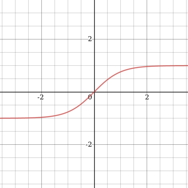
The hyperbolic tangent is very similar to the sigmoid. This is the correct sigmoid function, . Therefore, such a function has the same characteristics as the sigmoid we looked at earlier. Its nature is non-linear, it is well suited for a combination of layers, and the range of values ​​of the function is . Therefore, it makes no sense to worry about the values ​​of the activation function leading to computational problems. However, it is worth noting that the gradient of the tangential function has higher values than that of the sigmoid (the derivative is steeper than it is for the sigmoid). Whether we choose a sigmoid or a tangent function depends on the requirements of the gradient's amplitude. As well as the sigmoid, the hyperbolic tangent has the inherent vanishing gradient problem.

The rectified linear unit (ReLU), , returns if is positive, and otherwise:

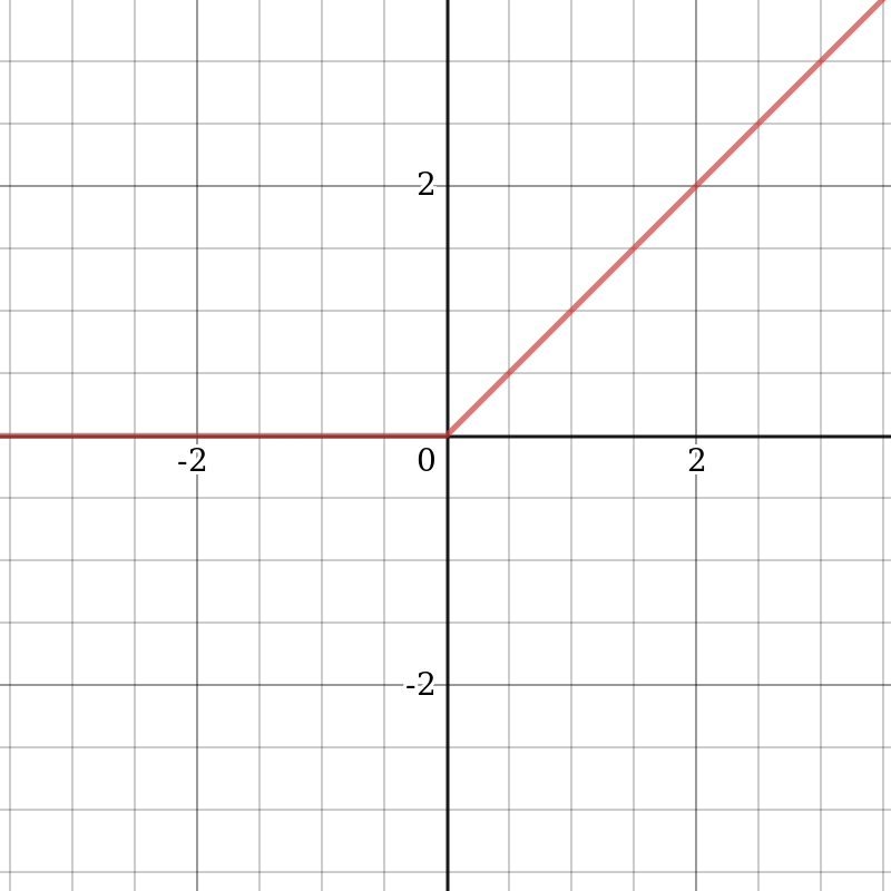
At first glance, it seems that ReLU has all the same problems as a linear function since ReLU is linear in the first quadrant. But in fact, ReLU is non-linear, and a combination of ReLU is also non-linear. A combination of ReLU can approximate any function. This property means that we can use layers and they won't degenerate into a linear combination. The range of permissible values of ReLU is , which means that its values can be quite high, thus leading to computational problems. However, this same property removes the problem of a vanishing gradient. It is recommended to use regularization and normalize the input data to solve the problem with large function values (for example, to the range of values [0,1] ).

Let's look at such a property of a neural network as the activation sparseness. Imagine a large neural network with many neurons. The use of a sigmoid or hyperbolic tangent entails the activation of all neurons. This action means that almost all activations must be processed to calculate the network output. In other words, activation is dense and costly.

Ideally, we want some neurons not to be activated, and this would make activations sparse and efficient. ReLU allows us to do this. Imagine a network with randomly initialized weights (or normalized) in which approximately 50% of activations are 0 because of the ReLU property, returning 0 for negative values of . In such a network, fewer neurons are included (sparse activation), and the network itself becomes lightweight.

Since part of the ReLU is a horizontal line (for negative values of ), the gradient on this part is 0. This property leads to the fact that weights cannot be adjusted during training. This phenomenon is called the Dying ReLU problem. Because of this problem, some neurons are turned off and do not respond, making a significant part of the neural network passive. However, there are variations of ReLU that help solve this problem. For example, it makes sense to replace the horizontal part of the function (the region where ) with the linear one using the expression . There are other ways to avoid a zero gradient, but the main idea is to make the gradient non-zero and gradually restore it during training.

Also, ReLU is significantly less demanding on computational resources than hyperbolic tangent or sigmoid because it performs simpler mathematical operations than the aforementioned functions.

The critical properties of ReLU are its small computational complexity, nonlinearity, and unsusceptibility to the vanishing gradient problem. This makes it one of the most frequently used activation functions for creating deep neural networks.

Now that we've looked at a number of activation functions, we can highlight their main properties.