
At the time of writing, for training neural networks nearly everywhere, the error backpropagation algorithm is used. The result of performing inference on the training set of examples (in our case, the set of subsequences) is checked against the expected result (labeled data). The difference between the actual and expected values is called an error. This error is propagated to the network weights in the opposite direction. Thus, the network adapts to labeled data, and the result of this adaptation works well for the data that the network did not meet in the initial training examples (generalization hypothesis).
In the case of a recurrent network, we have several options regarding which network outputs we can consider the error. This section describes the two main approaches: the first considers the output value of the last cell, while the second considers the outputs of all the cells from the last layer. Let's have a look at these approaches one by one:
- In the first approach, we can calculate the error by comparing the output of the last cell of the subsequence with the target value for the current training sample. This approach works well for the classification task. For example, if we need to determine the sentiment of a tweet (in other words, we need to classify the polarity of a tweet; is the expressed opinion negative, positive, or neutral?). To do this, we select tweets and place them into three categories: negative, positive, and neutral. The output of the cell should be three numbers: the weights of the categories. The tweet could also be marked with three different numbers: the probabilities of the tweet belonging to the corresponding category. After calculating the error on a subset of the data, we could backpropagate it through the output and cell states.
- In the second approach, we can read the error immediately at the output of the cell's calculation for each element of the subsequence. This approach is well suited for the task of predicting the next element of a sequence from what came previously. Such an approach can be used, for example, in the problem of determining anomalies in time series data, in the task of predicting the next character in a text, or for natural language translation tasks. Error backpropagation is also possible through outputs and cell states, but in this case, we need to calculate as many errors as we have outputs. This means that we should also have target values for each sequence element we want to predict.
Unlike a regular fully connected neural network, a recurrent network is deep in the sense that the error propagates not only in the backward direction from the network outputs to its weights but also through the connections between timestep states. Therefore, the length of the input subsequence determines the network's depth. There is a variant of the method of error backpropagating called backpropagation through time (BPTT), which propagates the error through the state of the recurrent network.
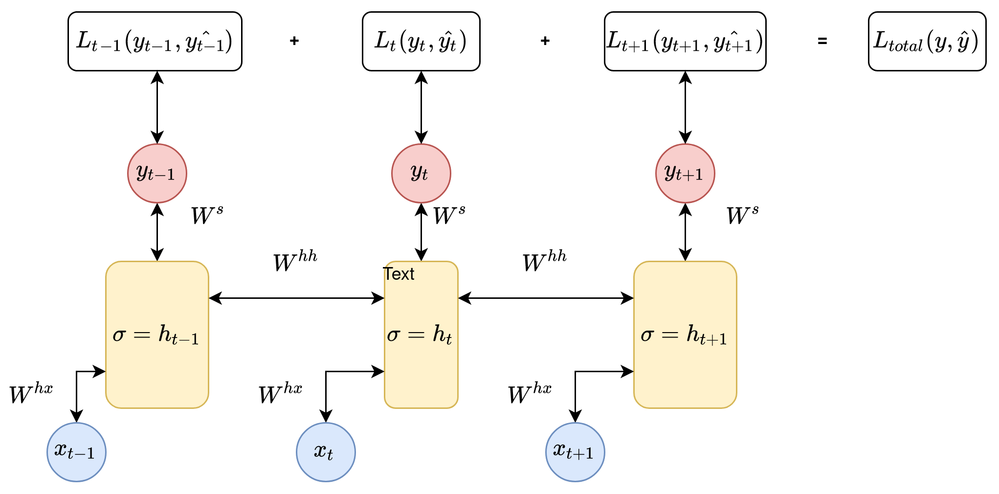
The idea behind BPTT is quite simple – we unfold a recurrent network for a certain number of timesteps, which converts it into a usual deep neural network, which is then trained by the usual backpropagation method. Notice that this method assumes that we're using the same parameters for all timesteps. Furthermore, weight gradients are summarized with each other when the error propagates in a backward direction through the states (steps). They are duplicated during the initial configuration of the network  times, as though adding layers to a regular feedforward network. The number of steps needed to unfold the RNN corresponds to the length of the input sequence. If the input sequence is very long, then the computational cost of training the network increases.
The following diagram shows the basic principle of the BPTT approach:
A modified version of the algorithm, called truncated backpropagation through time (TBPTT), is used to reduce computational complexity. Its essence lies in the fact that we limit the number of forward propagation steps, and on the backward pass, we update the weights for a limited set of conditions. This version of the algorithm has two additional hyperparameters: k1, which is the number of forward pass timesteps between updates, and k2, which is the number of timesteps that apply BPTT. The number of times should be large enough to capture the internal structure of the problem the network learned. The error is accumulated only for k2 states.
These training methods for RNNs are highly susceptible to the effect of bursting or vanishing gradients. Accordingly, as a result of backpropagation, the error can become very large, or conversely, fade away. These problems are associated with the great depth of the network, as well as the accumulation of errors. The specialized cells of RNNs were invented to avoid such drawbacks during training. The first such cell was the LSTM, and now there is a wide range of alternatives; one of the most popular among them is GRU. The following sections will describe different types of RNN architectures in detail.