11

Scratching the Surface of Shaders

Captain Edward J. Smith of the erstwhile and ill-fated ship the Titanic would no doubt be among the first to acknowledge the fact that the visible surface of an iceberg represents but a small fraction of an immensely greater object. When used as an analogy, the phrase “tip of the iceberg” is commonly understood to mean that what is visible, isn’t and shouldn’t be taken to be representative of the entire thing.

Note

The aforementioned, oddly specific call-out to Captain Ed Smith, is a fantastic Random Fact to know on Trivia Night.

Similarly, the idea of scratching the surface of a topic evokes imagery of kids attempting to dig a hole to the other side of the planet. Juxtaposed with a to-scale globe, it suggests the immensity of the digger’s undertaking. In no way does it diminish the enjoyment the children get from their quixotic adventure, but by depicting the differentiated layers of crust, mantle, and core, it acknowledges how a serious endeavor involves more than doing existing things on larger scales.

The preceding paragraph could come straight out of a self-help book with how hard it tries to hit its reader over the head with the analogy, but it does accurately describe the subject matter of this chapter. Shaders and programming for the GPU are the topics of this chapter in a broad sense, with a focus on the tools and how to use them in service of the topic. This leaves us with a problem like previous ones we encountered when we looked at input and control systems (Chapter 5, Adding a Cut Scene and Handling Input). As you may recall, the problem was that the amount of material needed to gain a solid understanding of the topic requires a book of its own to properly cover it!

As we did in previous instances, we’re going to cover as much of the fundamentals as possible while still laying the groundwork for whatever next steps you decide to take in learning this subject. This means that there might be things that don’t get a whole lot of space, but that will be made up for (hopefully) by the excellent links and resources that are available and listed.

In this chapter, we will cover the following topics:

• Understanding Shader Concepts
• Writing and Using Shaders in Babylon.js
• Shader Programming with the Node Material Editor

This is a far more limited number of topics than what could have been covered, but by the end of this chapter, you’ll know enough to be immediately productive in current projects while also having enough grounding to see where your next steps in learning lead.

Technical Requirements

The technical requirements for this chapter are the same as the previous ones; however, there are some subjects and areas that might be useful to refresh or catch up on:

• Vector math operations: This includes addition, subtraction, dot, cross, and others. You won’t need to perform the calculations or memorize any equations, but knowing the significance or purpose of them (for example, you can use vector subtraction to find the direction between two objects) is the key to making the knowledge useful.
• Function graphs: Both Windows and macOS have built-in or freely available graphing calculators that can graph entered equations. This is useful in understanding the output of a piece of shader code across varying inputs. Graph like it’s TI-89! An online-only option is the Desmos Graphing Calculator at https://www.desmos.com/calculator.

Understanding Shader Concepts

In the days before standalone GPUs were commonplace, drawing pixels to the screen was a lot different than it is today. Kids these days just don’t know how good things have gotten with their programmable shaders! Back then, you would write pixel color values directly into a buffer in memory that becomes the next frame sent to the display. The advent and proliferation of the dedicated graphics processor as an add-on came in the late 1990s, and it changed the landscape completely. Access to display pixels was abstracted around two major Application Programming Interfaces (APIs): DirectX and OpenGL. There’s an incredibly rich history of the evolution of those interfaces but this isn’t a book on graphics hardware interfaces and their history – it’s a book on present 3D graphics development, so let’s just leave the details to those tomes and summarize them in short.

To avoid the need for developers and end user software to support every model and make of graphics cards, a set of APIs was developed that a hardware manufacturer could then implement. Two competing standards emerged – DirectX and OpenGL – and for the subsequent decade or so, drama ensued as each tried to adapt and change to a rapidly evolving graphics technology landscape. We’re going to finish this section by looking at shaders themselves, which requires us to understand how a shader relates to the rest of the computer hardware and software. Before we can understand that aspect, however, we need to understand why it’s important to make these types of distinctions in the first place.

Differences Between a GPU and a CPU

A graphics processor isn’t built the same way as a regular CPU. At a fundamental hardware level, a graphics processor is built around performing certain types of tasks very fast. This meant that applications needed to contain specialized code that could leverage these capabilities to their fullest. As opposed to code that you may typically write for the frontend or backend of a website, where code is executed sequentially, one instruction after another, a GPU wants to execute as many operations in parallel as possible. Still, this is not an illuminating way to describe how a GPU is programmed differently from how we may know from previous experience and intuition. A better analogy might be in thinking about how a painter might render a large mural onto a wall, as seen in Figure 11.1.

Like traditional programs, most printing that people are familiar with at the consumer level is done by a process known as rasterization – a print head scans the paper, spraying down ink of specific colors at times and places it corresponding to the patterns of colors of the print. In this way, a picture is progressively built from one corner to its opposite, line by line, pixel by pixel. Our painter works similarly, starting from one part of the painting and building up the mural piece by piece:

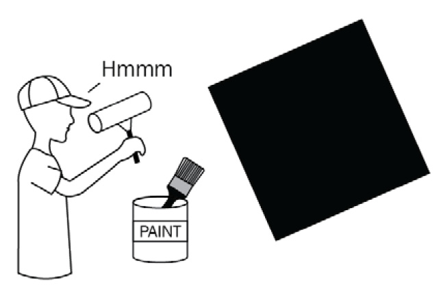
Figure 11.1 – An analogy of traditional computing has a single painter working on the entire portrait themselves as being analogous to how a CPU processes instructions

In contrast to our lone painter-as-a-CPU, graphics processors ditch the raster process and go with a more distributed shotgun approach to painting an image. Here, thousands of painters are all assigned to work on different small slices of the same piece. None of the individual “painters” has any knowledge about what their brethren are up to; they just have their instructions for painting their tiny piece of the full picture:

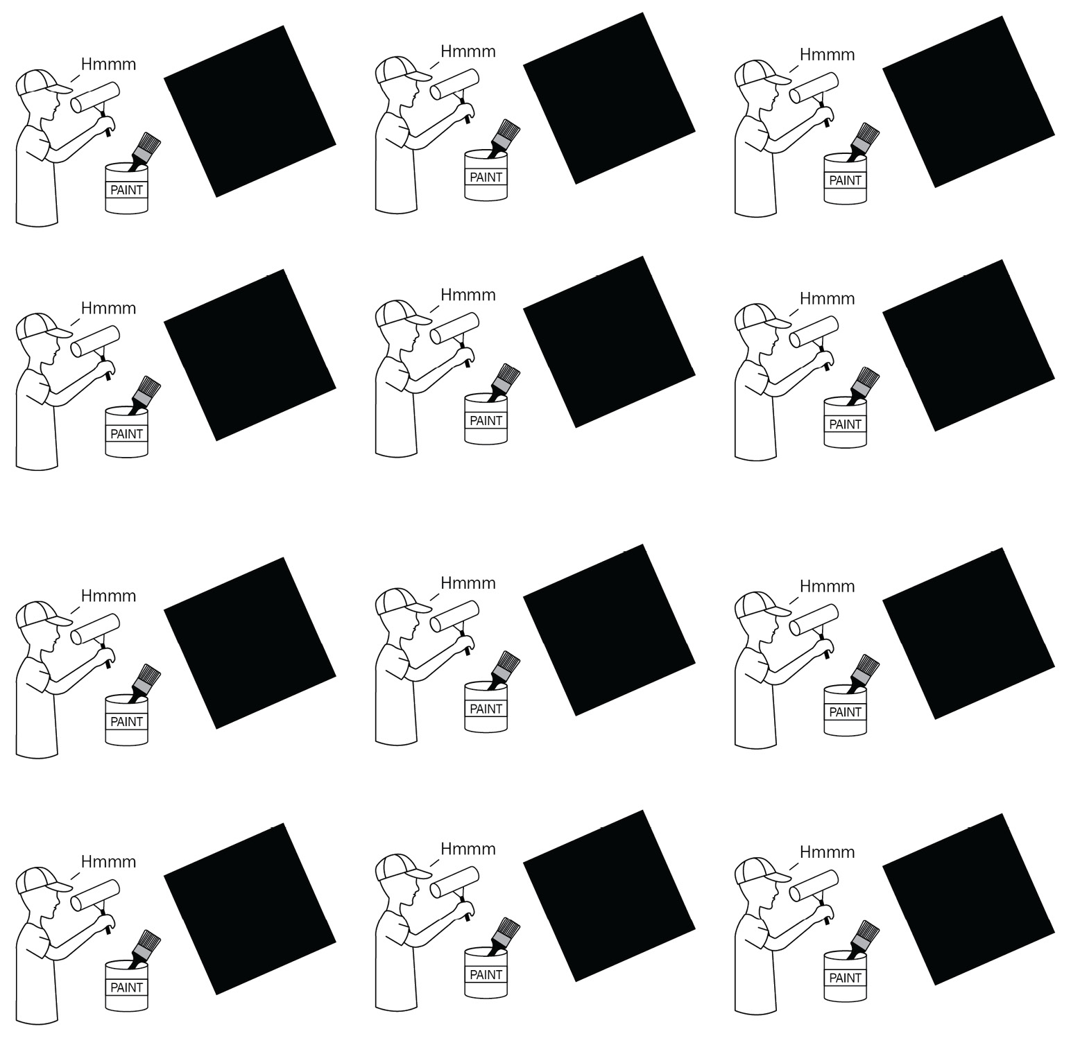
Figure 11.2 – Graphics cards execute instructions simultaneously, with each “painter” getting only a tiny piece of the full canvas to work on, and with no knowledge of any other painter

It is in this manner that graphics cards can handle the billions of calculations per second needed to drive modern 3D graphics applications and games. As the previous diagram implies, instead of a single painter (processor) methodically laying down each line and each layer of paint until the picture is complete, there is a legion of painters that each execute the same set of instructions, but with data wholly specific to their part of the canvas.

Shaders are GPU Applications

How can applications take advantage of this way of processing? More importantly, how can a developer write code that takes advantage of this massively parallel processing resource? To answer those questions fully and with the appropriate context would (again) require an entire book of its own. The Extended Topics section of this chapter contains several such excellent tomes! We will leave historical context, fundamental concepts, and the hard mathematics to those more worthy voices and instead focus on more practical aspects of writing the instructions handed to those legions of painters in the form of graphics card programs, more commonly referred to as shaders.

In the graphics rendering process, we start with various data from the Scene, such as geometry, lighting, and materials, and we finish with a frame displayed on the screen. This result comprises a collection of pixels and their colors, one pixel/color combination for every point displayed on the screen. In the space between the Scene and the Screen, there are several important steps, but at a high level, this is the Rendering Pipeline:

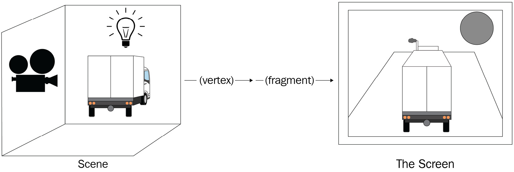
Figure 11.3 – Simplified rendering pipeline. Starting with the Scene as initial the input, sequentially executed shader programs convert the scene geometry into pixel locations, and then finally pixel locations into colors

Each step of the pipeline receives input from the previous steps’ output. The logic specific to each step that we’re interested in is handled and represented by an individual shader program. However, recall that in this context, an individual shader program is a piece of code that will be executed in a massively parallel fashion, with the data relevant to each part of the screen or scene making up the inputs and the processed equivalents of their outputs.

About Shaders

As mentioned earlier, a shader is a type of executable program that runs on the GPU. The shader program is provided a set of constants, or uniforms, that contain the input data that can be used by the shader. Shaders can also reference textures as input for sampling purposes – a powerful capability we’ll exploit later in this chapter. Some examples of common uniforms are animation time multipliers, vector positions or colors, and other data useful in providing configuration data to the shader. The output of a given shader varies; for a vertex shader, the output is the given geometry’s projection from world to screen space at the vertex level. A fragment shader’s output is completely different – it is a pixel color value. Something more advanced is a WebGPU Compute shader, whose output can be arbitrary – later in this chapter, we will look at this more closely!

The shader program types we’re going to be working with here fall into two categories: Vertex and Fragment. Although they’re being introduced as separate things, they are usually contained and defined within the same shader code. Two main languages are used to write shader programs in use today: Hardware Lighting and Shading Language (HLSL) and OpenGL Shader Language (GLSL). The first, HLSL, is used by the Microsoft DirectX graphics API. We’re not going to spend any time on HLSL because WebGL, WebGL2, and WebGPU (with a caveat; see the following Note) all use the second language, GLSL. Since Babylon.js is built on a WebGL/2/GPU platform, GLSL is what we’re going to focus on in our brief overviews.

Note

WebGPU uses a variant of GLSL called wGLSL, but because Babylon.js is so focused on maintaining backward compatibility, you have the choice to use wGLSL or continue writing shaders in regular GLSL – either way, you can still use WebGPU thanks to the way Babylon.js transpiles shader code. See https://doc.babylonjs.com/advanced_topics/webGPU/webGPUWGSL for more information on wGLSL and Babylon.js transpilation features.

Both HLSL and GLSL are syntactically related in flavor to the C/C++ family of programming languages, and though JavaScript is a much higher-level language, there should be enough familiar concepts for people familiar with it to gain a good starting position for learning GLSL. Coming from JavaScript, it’s probably the most important to keep in mind that, unlike JS, GLSL is strongly typed and doesn’t like trying to infer the types of variables and such on its own. There are other quirks to keep in mind, such as the need to add a . suffix to numbers when a floating-point variable is set to an integer value. This is a good segue to talk a little bit more about how shader programs are different from other software programs.

Shaders, as a class of software, have several distinctive features:

• They are stateless. Because a given graphics processor (of which a graphics card might have thousands or millions available) might be tasked with rendering Instagram pics one moment, it could just as easily be rendering an email or text document the next. Any data needed by the shader, whether it’s a texture, a constant, or a uniform, must be either defined within the shader itself or passed into it at runtime.
• There is no access to shared state or thread data – each process stands alone, executing with no knowledge of its neighbors.
• Shader code is written to address the entire view or screen space, but the instructions that are given to each instance must be formulated in such a way that each instance gets the same directions yet produces the desired individual results.

Between the first two items causing the third is the genesis of the reputation for the fiendish difficulty that shaders have gotten. Like everything, writing shader code is something that requires practice. Eventually, with practice, it will become easier and easier to slip into the shader mindset and solve increasingly more complex and difficult problems; you’ll soon be wondering what all the fuss was about! In the next section, you will learn about a few of the different ways to incorporate a custom shader into a project. Again, don’t sweat the next section too much if this is outside of your comfort zone – let it soak through you. The concepts we’re covering here will be useful later when we learn how to use the Node Material Editor (NME) to do all the heavy lifting of writing shader code while you focus on what you want to get done.

Writing and Using Shaders in Babylon.js

Being that shaders are defined using plain text, there are a lot of different ways to store and load shaders in a project. We’ll review some of the ways to accomplish this after we learn a bit about how shader code is structured. The Create Your Own Shader (CYOS) tool is the shader equivalent of the Babylon.js Playground and is just one way to write shader code for Babylon.js. Navigating to the CYOS URL at https://cyos.babylonjs.com shows the shader code on the left pane and a live preview of the output on the right:

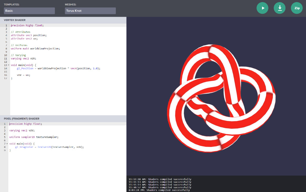
Figure 11.4 – The Babylon.js Create Your Own Shader tool functions similarly to the BJS Playground

In the preceding screenshot, you can see that the shader code is defined for vertex and fragment shaders in the left-hand pane, while a live preview shows on the right. Starter templates can be selected from the dropdowns, along with different meshes to use in the preview.

Just like the Playground, you can save your work to a snippet server, or you can download a ZIP file containing the shader code embedded into a template HTML file. Also, just like the PG, the Play button compiles and runs live the results of your shader programs. That’s the overall mechanics and usage of the tool. Now, let’s see how it fits into what we’ve been learning about the different types of shaders.

Fragment and Vertex Shaders

Let’s remind ourselves of what the top section, the Vertex shader, and the bottom, the Fragment shader, do in this context. The Vertex shader is relevant only when there is mesh geometry involved, which means that Vertex shaders must be applied to a mesh. In other words, this is what we’d call a Material. Fragment shaders determine the color of a vertex fragment (for Meshes) or pixel (procedural textures, post-processes). They can stand alone, such as when they are used for a Post Process, or with Vertex shaders in a Material. Like our JavaScript code files, a shader program consists of a set of different types of declarations. Instead of a constructor function and the like, a shader program is required to have at least a definition for the void main(void) function because that is the function that is executed by the GPU. Outside of the main function, subroutines or helper functions are commonly used to help encapsulate and isolate code, just as you would do with any other well-written code that you may write. Inputs to the shader are specified at the top along with other declarations. Depending on the type of shader and how it is defined, there might be several different arbitrary declarations present, but two that are always provided are the position and uv attribute declarations. The former is a Vector3, while the latter is a Vector2; both represent data coming from the source mesh geometry:

• The local space position of the vertex is the coordinates relative to the mesh origin, not the world origin.
• The uv attribute is the texture coordinates. It is so-called to avoid confusion with the xy coordinates outside of the texture space.

Other declarations include the following:

• A uniform four-by-four Matrix called worldViewProjection that contains the transformations needed to convert the vertex position from local into World and then into View (screen, or 2D) space.
• A varying (reference type variable capable of being mutated or changed) vUV. This is one piece of (optional) data that’s passed to the fragment shader. It’s important for looking up pixel colors from a sampled texture.

The output of the Vertex shader is a Vector3, in the form of the gl_Position variable, and must be set in the shader before reaching the end of main. Its value is computed by applying the provided matrix transformation to the vertex position after any custom computations have been applied to the position value.

Important note

A lot of detail about these concepts isn’t being covered here because otherwise, we wouldn’t be able to cover everything about other topics. However, these basics should be enough to help you start being able to read and understand shader code, and that’s the first step to attaining proficiency!

The bottom part of the CYOS screen’s code panel is where the Fragment shader lives. Instead of receiving the vertex position of a mesh, the fragment shader receives a 2D screen position in the form of varying vUV and outputs a color to gl_FragColor. This color value represents the final color of the current pixel on the screen. When using textures with shaders, textureSampler references a loaded texture in the GPU memory, with the texture coordinates vUV used to look up the color value. These coordinates can be supplied by the mesh geometry (in the case of a material), view or screen coordinates (for post-processes or particles), by some computational process (as is the case for procedurally generated digital art), or with some combination of all three techniques. Change the dropdown selector labeled Templates to see more examples of how you can use shaders for fun and profit!

Compute Shaders (New to v5!)

The availability of programmable shaders exposes the power of the modern GPU to everyday desktop applications. With the latest WebGL2 and WebGPU standards becoming more and more commonly implemented by major web browser vendors, that power is now available to web applications too. The biggest WebGPU feature when it comes to shaders is a new generation that’s intended for general-purpose computation, called the Compute shader.

For specific documentation on how to write and use WebGPU Compute shaders, go to https://doc.babylonjs.com/advanced_topics/shaders/computeShader. Vertex and fragment shaders are purposefully limited in the extent and scope as to what they can accomplish, especially when those tasks don’t directly involve Scene geometry. Compute shaders, on the other hand, are a way to run more arbitrary – though no less massively parallel – calculations and output. Let’s look at a concrete example of the types of problems that Compute shaders are good at solving.

In this scenario, we want to simulate the effects of water erosion on terrain. Things such as an ocean tide besieging a sandcastle or long-term weathering of mountains are more accurate when the underlying calculations have finer resolution – more particles involved means that each particle can represent a smaller and smaller piece of the overall fluid volume. There are a few things that make this scenario quite nice for Compute shaders. When modeling fluids, approximations are used to simplify calculations. As mentioned previously, the number and size of the individual calculation units are directly tied to the overall accuracy and performance of the simulation. If the simulation were a mural, the speed it is painted and the resolution or detail depend on how many “painters” are assigned to handle painting the mural. What makes a Compute shader the ideal choice is that vertex and fragment shaders have more limitations on how many, what types, and which data can be updated, whereas Compute shaders are capable of writing output (similar to a texture) that isn’t displayed directly onto the screen. They even make passing data back to the CPU from the GPU more practical, although it is still not a great idea if you can avoid it – passing any data in that direction will always be a slow operation. Additionally, the increased computing power makes more accurate but computationally intensive calculations available.

This may not seem like a big deal, but it is. Being able to persist and then reference output of and from a compute shader allows for a huge amount of utility – it’s like Inspector Gadget and his signature catchphrase. Yell “Go Go Gadget Compute shader!” and anything can happen! The output from a compute shader can be used to drive a terrain height map, compute the values of a vector field, and much more.

Note

See https://playground.babylonjs.com/?webgpu#C90R62#12 to learn how to use a Compute shader to simulate erosion with a height map and dynamic terrain. Note the addition of webgpu to the query string – running WebGPU samples requires a browser with WebGPU support. As of April 2022, only Chrome and Edge Canary builds support WebGPU features. See https://github.com/gpuweb/gpuweb/wiki/Implementation-Status to view the latest implementation support and status in Chromium-based browsers.

Compute shaders require WebGPU and carry with them a great deal of complexity, but some problems are worth that added complexity. Able to perform massive numbers of calculations in parallel, Compute shaders are different from vertex or fragment shaders because they can write to textures or other storage buffers to read and write values from that can then be used by other processes in the rendering pipeline. Still nascent in its eventual ascendancy to widespread adoption and replacement of WebGL2, and with support only beginning to appear in major web browsers, WebGPU and Compute shaders are technologies worth getting familiar with sooner rather than later.

Continuing the Shader Code Journey

It mentioned earlier, the topic of shaders is a vast and complex enough topic to warrant its own book rather than just a chapter. Fortunately, books such as those do exist, and one of the best is The Book of Shaders, by Patricio Gonzalez Vivo and Jen Lowe. Completely free and accessible at https://thebookofshaders.com, The Book of Shaders describes itself as “a gentle step-by-step guide through the abstract and complex universe of Fragment shaders,” and it’s a case where the description closely matches reality. As it says, the book focuses on Fragment shaders only, but its wider value comes from the immersion and practices it provides for thinking in shader code. Filled with self-executing examples and exercises, it won’t take long to start having fun and being productive with shaders!

Let’s recap on the different types of shaders and what they are used for with this handy table:

With how easy WebGL2 makes it to expose shader logic and GPU features in the web browser, there are many tools and resources to explore in your journey of learning shaders. Maybe your experience is more on the design and art side of things, and the idea of writing code could be intimidating or otherwise off-putting in some way. Perhaps it’s simply difficult to keep in mind both the goal of what you want to accomplish while holding the concepts of vertex and fragment shader syntax. Or it could be that you’re unsure of how to write a particular shader effect and need to experiment and explore to discover how to proceed. All these reasons, plus many more not listed, are good reasons to take a good long look at one of the flagship features of Babylon.js: the Node Material Editor (NME). This is what we are going to do in the next section.

Shader Programming with the Node Material Editor

As something that has been referred to numerous times throughout this book, the NME may have taken on an almost mythic status as a productivity tool. Its plug-and-play, drag-and-drop nature allows just about anyone to assemble shaders using visual blocks. It democratizes the GPU in the seamless way it integrates with the Inspector. Its simple deployment in tandem with the Playground provides a short runway from fancy to flight. The NME may just be about the best thing to happen since sliced bread met butter.

All these statements are true, except the part about the NME being better than sliced bread and butter – that one isn’t. It’s better than sliced bread and butter, falling just short of being better than sliced bread alone. It’s a thin leavened line, but it’s one worth baking. Hyperbole aside, the NME is truly one of the most powerful, if not the most powerful, tools in the Babylon.js toolbox.

In this section, we’re going to learn how to get the most out of the NME. By the end, you’ll find it easy to “think in nodes”! First, we’ll explore how to create and apply a NodeMaterial to a mesh. Next, we’ll explore using the NME to create procedural textures. Finally, we’ll wrap things up with a quick look at how to use NME to create a Post Process.

Using the NME to Build the Planet Earth Material

Sometimes, when learning something new, it can be helpful to have a concrete example to work toward, with the example being the end goal to reach. Other times, it can be more illuminating to begin not with the example of a finished product, but with an atomic subset of that final goal. The goal we’re going to start with – our first atomic subset – will be simple: create a new NodeMaterial that renders a texture onto a sphere mesh. Easy, right?

Note

Unlike most rhetorical questions framed similarly, the answer to the preceding question is an unambiguous, full-throated “YES!”. If it isn’t already apparent that Babylon.js places an incredibly high emphasis on ease of use, it would be helpful to go back and re-read (or simply read for the first time) the previous chapters of this book. It’s OK, no one’s judging you for skimming or skipping! Well, OK. Maybe a little bit. But not much.

As we work through this chapter, we’re going to start by covering a lot more details on the mechanics of how to accomplish various tasks with the NME, but as we make progress through the following sections, we’ll have to start zooming out from those mechanical details to make sure we leave enough space and time for bigger-picture topics. As always, the Babylon.js docs are a great place to learn more about the topics we’re covering, with great material on the NME that includes combination Playground and NME examples for a wide variety of tasks. The BJS forums are a great place to view examples from the community, as well as to solicit feedback and ask questions. There’s even a thread dedicated to NME examples at https://forum.babylonjs.com/t/node-materials-examples! Let’s get started.

NME Overview

Navigate to https://nme.babylonjs.com; the default material mode “blank slate” is the initial node graph to be loaded. Broken down into four functional areas with a fifth preview pane, the first pane – the left-hand side vertical column – hosts a searchable list of different nodes that can be placed into the center pane of the work canvas:

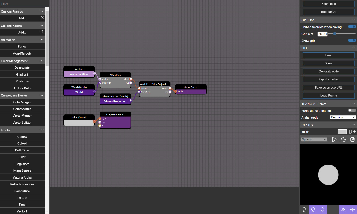
Figure 11.5 – The default Node Material Editor view

In the preceding screenshot, the left-hand pane contains the list of nodes. The center pane work canvas is where nodes and their connections are displayed, while the right-hand pane shows contextual properties for the selected item. Note the render preview pane.

The right-hand pane displays a contextual list of properties that can be modified, or if nothing is selected, the snippet properties and options. Tucked into the bottom (scroll down if it’s not visible initially) of the Property pane is the Preview panel. Pop that out into its own window right away – being able to immediately see the effects of making a change is one of the keys to success in this type of development. The bottom well or gutter, depending on how you want to term it, contains console output from the shader compilation process of the node graph – if the bottom line is red, then your nodes aren’t compiling!

Important note

Sometimes, it can be tough to tell if a particular change is extremely subtle or whether it has no effect at all. Always make sure to check that your most recent console output isn’t colored red or contains an error; otherwise, you may mistake a broken node with an ineffectual change!

Background Context

Nodes are connected by lines between specific connector ports on the two involved nodes. Any given node represents a particular operation that can be performed on a series of inputs and outputs, connected by dragging lines from the former to the latter. The graph of nodes and their connection follows two simple rules that result in strikingly complex behaviors.

First, nodes always accept input on the left-hand side connectors and output values on their right. What happens inside the node between the input and output is nobody’s business but the nodes’. An interesting implication of this is that uniforms, attributes, constants, or other externally provided data do not have input connectors. Rather, values are set via code, the Inspector, or at design time in the property pane. Conversely, a few nodes only contain inputs and have no output connector. These are the endpoints for the node’s shader code generation; in other words, they represent the return value of the applicable shader, such as a color for the fragment shader and a position vector for the vertex. Since they are the final result of the shader calculations, they must always be the last item in the node graph.

The second rule for node graphs, and following from the first, is that only nodes connected to an output node are included in the generated shader code. Remember, the final goal is to generate a vector for the vertex shader and a color for the fragment. This means that a properly formed node graph executes a sequential path from start to finish (usually left to right), but which is defined by that path traced from end to start (the opposite, or right to left).

This mismatch in mental models (try saying that five times fast!) can sometimes make it difficult to visualize the steps needed to get to a particular goal line. That’s why it’s important to make things easy to change or add to without having to make unrelated changes to the application that are needed just to be able to make a change. In our case, we’re going to structure our work so that we can incrementally build an ultra-high detail and quality Planet Earth material.

Back to the NME window, drag out the fragment and vertex output nodes out to the right to make room for the new nodes we’re going to add. Make sure that the render preview is set to Sphere, and while you’re at it, pop the preview out into a separate window if you haven’t done that yet. Now, we’re ready to accomplish our first micro-goal of learning how to add and use textures.

Adding a Texture to the Material

In the default configuration for the Node Material Editor’s Material mode, the inputs for the vertex shader are mesh.position, World Matrix, and View Projection Matrix. A series of TransformBlock nodes connect the inputs to form the final vertex position. Click in the search pane of the left-hand node list and start typing the word texture to filter the list down to display the Texture node of the Inputs group, then drag it out onto the surface somewhere. You’ll see the Texture node appear, but if it isn’t already present on the canvas, an additional Vector2 mesh.uv node hooked up to the uv connector of the Texture block will be created. In general, this is a consistent pattern – if the required inputs for a node block aren’t present, they will be added automatically:

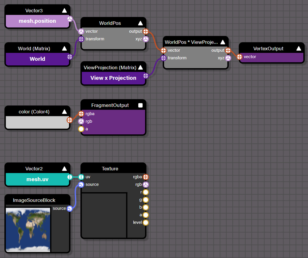
Figure 11.6 – Dragging the Texture node onto the surface also adds the mesh.uv value. This is used to select the portion of the texture corresponding to the mesh vertex

The preceding screenshot shows the setup, but it also shows our next step: dragging out the source input port on the Texture block to create a new ImageSource node. An ImageSource is an important piece of indirection that allows a node material to separate the process of loading a texture from the data contained in it. Advanced usage scenarios can involve using a Render Target Texture (RTT) to obtain a rendered texture of a mesh before performing additional processing. Click the Image Source node. Then, in the Link property textbox, upload from your local repository or provide this URL: https://raw.githubusercontent.com/jelster/space-truckers/develop/assets/textures/2k_earth_daymap.jpg (it’s up to you!). The image should load into the Texture block, as depicted in the previous screenshot. It’s a good practice to tidy as we go along, so rename the node by selecting the node if it isn’t already and changing the Name property to baseTexture. Half of our initial objective has now been achieved by bringing in the texture. Now, we need to paint it onto the preview mesh.

Accomplishing this is incredibly easy, but it’s valuable to remember the underlying mechanisms involved since they will be important soon. Recall that the vertex shader is passed the mesh position and a UV texture coordinate corresponding to that vertex location, which passes the UV coordinates into the fragment shader. Now, we need to sample the texture to set the fragment shader’s final color, and we do that by dragging the rgb output of the baseTexture node to the rgb input of the FragmentOutput node. Look at the Render Preview; a familiar-looking globe should be visible:

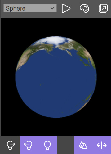
Figure 11.7 – The Render preview of the Planet Earth material after adding baseTexture and sampling it for FragmentOutput

You can check your work-in-progress against the snippet at #YPNDB5. If your preview doesn’t match the preceding screenshot perfectly, it’s OK – it’s just a preview at this point and the important thing is that you can see the texture on the sphere. Our first mission is accomplished! What’s next? It’s time to start adding nodes to our graph that will use additional textures to add further detail to our Planet Earth material.

Mixing Clouds

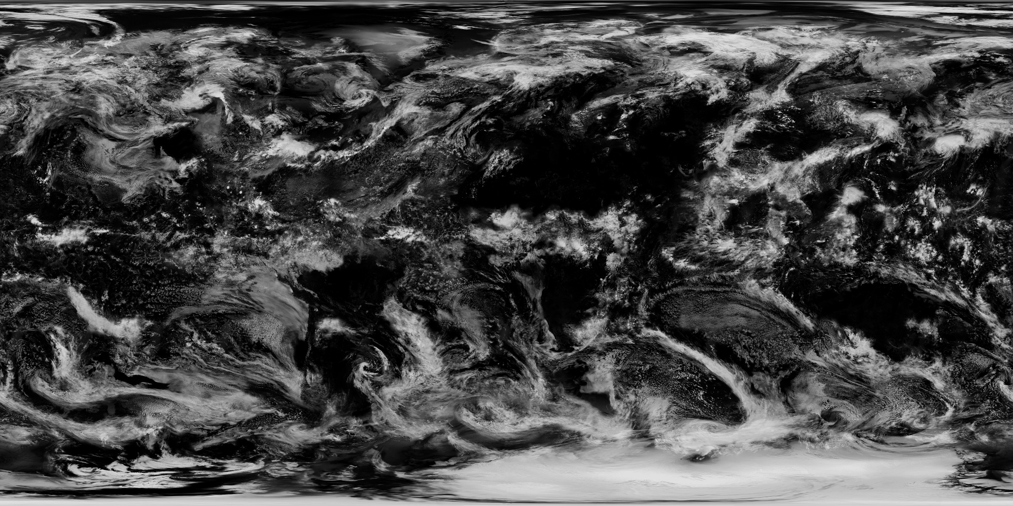
Start by adding another Texture node and ImageSource to the canvas. Name them cloudTexture and cloudTextureSource and upload or link to the file at https://raw.githubusercontent.com/jelster/space-truckers/develop/assets/textures/2k_earth_clouds.jpg to load the cloud texture into the design surface. The simplest way to get the clouds overlaid on top of the base texture is to add the colors from each texture, so drag an Add block out onto the surface and name it Mix Cloud and Base Textures. This highlights an important property of nodes that may catch those who aren’t familiar with this type of editing surface off guard – type matching.

When the node is initially added to the canvas, both the input and output ports are a solid red color, indicating that the type of input and output has yet to be designated. In this case, the possible types could include a Vector of 2, 3, or even 4 elements (or a color comprised of the same number), a single scalar number, or even a matrix. Which type the block turns into depends on the first connection made to the node. Connect the rgb ports of the two textures to the separate inputs of the node and replace the fragment shader’s output with the output from the Mix Cloud and Base Textures node to finish the operation. The clouds are visible on the render preview, but they’re a bit faint and hard to see.

This can easily be fixed by applying a scaling factor to the cloud color before it is mixed with the base texture color. This mixing of colors is a very common operation, especially more so when we move on to the next section, Procedural Textures and the NME. Add a Float input block and name it cloudBrightness. Give it an initial value of 1.25 or so and then use it as the input factor to a new Scale node that you’ll also add to the canvas. Name that node Scale Cloud Levels and connect the other input to the output of the cloudTexture node. The output of the Scale Cloud Levels node replaces the input to the Mix Cloud and Base Textures node:

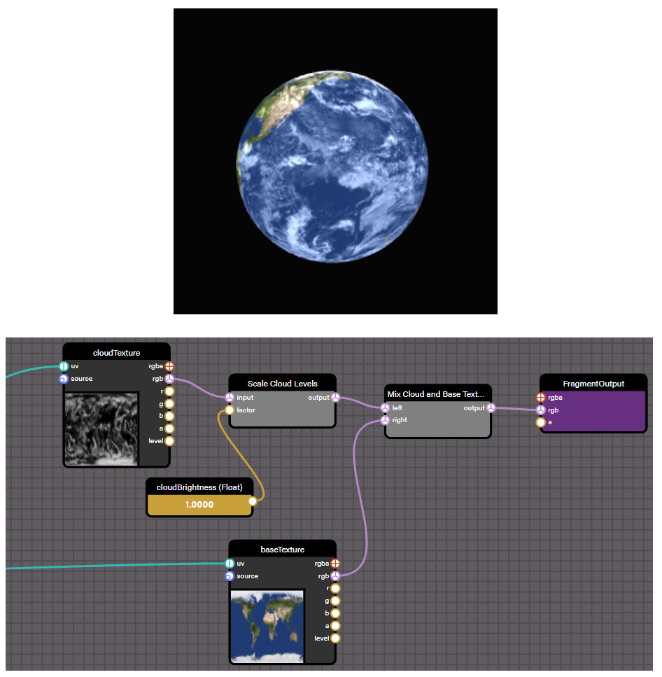
Figure 11.8 – (a) After adding the cloud texture and a scale factor to the base texture color, clouds can be seen floating over a serene Planet Earth. (b) The node material graph for mixing and scaling the cloud texture with base Earth texture. The cloudBrightness value can be set to a value that matches the desired look and feel of the clouds

The result should look like the first screenshot. If it doesn’t, compare your node graph to the second screenshot or to the snippet at #YPNDB5#1 to see what might be different between them. Once you’re happy with the output, it would be a good idea to save the snippet as a unique URL.

Note

While working on something with the NME, it’s quickest to save snippets as URLs until you are ready to download the definition file and use it in your project.

Our Planet Earth Material is looking pretty good now, but what is cooler than a boring old static texture? An animated texture! Let’s animate the clouds to give our material some life.

Framing Animations

When we think about animations, it’s easy to forget that there are many different methods of animating things in a scene. One of the simplest, most straightforward means is to manipulate the texture coordinates (the uv value) over time. Furthermore, by changing just the u (or X-axis) value, the texture will be shifted in an East-to-West or West-to-East fashion, similar to how it might look for a geostationary satellite!

Search for and add a Time node to the canvas. This represents a built-in shader input that provides the amount of time since the scene was started, in milliseconds (ms). We can use this value to drive our animation, and by multiplying it with a scaling factor float input of timeScaleFactor in the scaleSceneTime node, we can control the precise speed of the animation at design and runtime.

Important note

Why are we using Time instead of Delta Time? Remember, shaders have no memory of past events. They only deal with the data passed in, and the data passed in doesn’t persist between frames. Therefore, instead of storing the delta time and adding it to the u coordinate, we use total scene time and scale.

It’s important to keep a node graph readable, as much for your future self as for others reading it. One great way to do that is to organize nodes into collapsible Frames. Arrange the three Time, scale, and Multiply nodes close to each other, then hold down the Shift key while clicking and dragging a box around the three nodes to create a Frame:

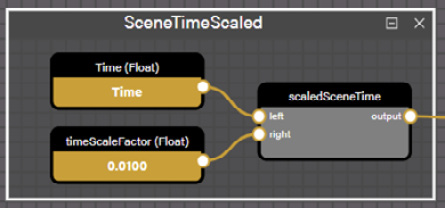
Figure 11.9 – The SceneTimeScaled frame encapsulates the logic for exposing an animation frame counter to the rest of a node graph. This is the expanded form of the frame

Frames are an easy and fast way to make a complex node graph more manageable, much as a function helps to separate and isolate pieces of code from each other. The SceneTimeScaled frame (or any frame) can even be reused across different Node Materials by downloading its JSON definition, then using the Add… functionality in the left-hand node list. Now, it’s time to make some movement by hooking up the output from the frame to the cloudTexture U coordinate.

Unlike when we mixed the cloud texture with the base texture where everything involved is of the same type, we need to be able to change a single element of a Vector2 value. First, we’ll need to split the source vector into its components before adding the scaledSceneTime value to the x component. Then, we’ll recombine the Vector and hook it into the cloudTexture UV input:

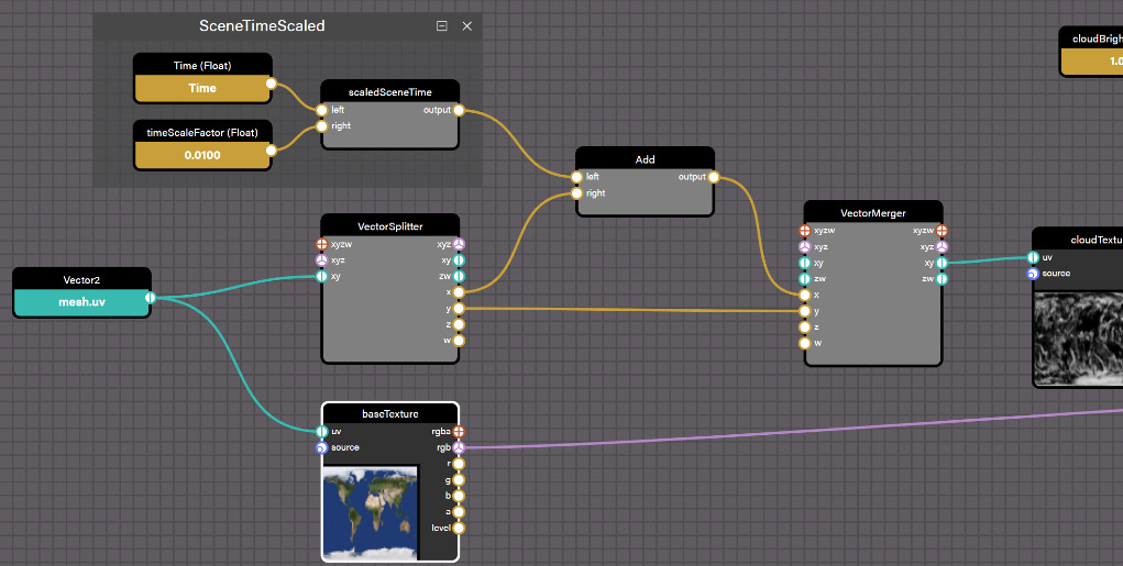
Figure 11.10 – Connecting the SceneTimeScaled frame with the u (x) texture coordinate using the Vector merger and Vector Splitter nodes

When this is connected, pull up the render preview and marvel at the slowly moving banks of clouds over serene blue oceans. If you don’t see the expected results, check the output well to make sure the last (current) line isn’t an error or in red. If needed, compare your NME graph with the one at T7BG68#2 to see what you’re doing differently.

There’s much more to the NME material mode than what we’ve accomplished in just a few short paragraphs. In that short span of text, we were able to create a nice render effect of an animated Planet Earth globe using the NME in Material Mode and with high-resolution textures provided by the kind folks at NASA. Dragging nodes out onto the canvas is fast becoming a familiar activity as we learned how to mix textures into a final Fragment Color, and even animate the cloud cover. Using built-in Time counters and Vector Splitter and Merger nodes will become second nature to us with practice and experience. There’s more to be covered than just how to map a texture onto a mesh with the NME, though. In the next section, we’ll take away the Vertex shader and focus on the Fragment shader as we finally learn how our Radar Procedural Texture is built (see Chapter 9, Calculating and Displaying Scoring Results, for more information on how this fits into the game).

Procedural Textures and the NME

In most specialized fields of study, a particularly hard foundational subject for the field at hand is often given to students early on in their journeys to weed or wash out students from the program. It sounds harsh, but exposing pupils early on to the realities of their chosen field can be a valuable way to save time and effort on both the students’ and teacher’s behalf. This part of the chapter is not intended to have that effect because presumably, you’re here by choice and by interest, and this isn’t a gatekeeping exercise, it’s an inclusive one. The Procedural Texture mode of the NME will still contain the vertex shader output – and it is still required to be present on the canvas – but our attention will be focused on the Fragment shader, because what else is better equipped to process a bunch of arbitrary pixels all at the same time than the Fragment shader? Nothing! In the case of procedural textures, the Fragment shader outputs to a texture buffer instead of the screen buffer – which is what a post-process uses. That texture, as we’ve seen with the Radar texture, can then be applied to various material texture slots in the scene for rendering.

It is in that regard and spirit that the node graph for the Radar Texture should be accepted – not as a scarecrow to frighten off those who might be less confident but to bolster and support those people. That’s why we’ll start with the simplest depiction of this node graph that still conveys the essentials. The reason for this is that while there are a decent number of moving parts involved in making this texture, each is fairly easy to understand once broken down. Follow along with the text by loading up snippet XB8WRJ#13 in the NME. Refer to the following diagram for notes on each specific component of the texture:

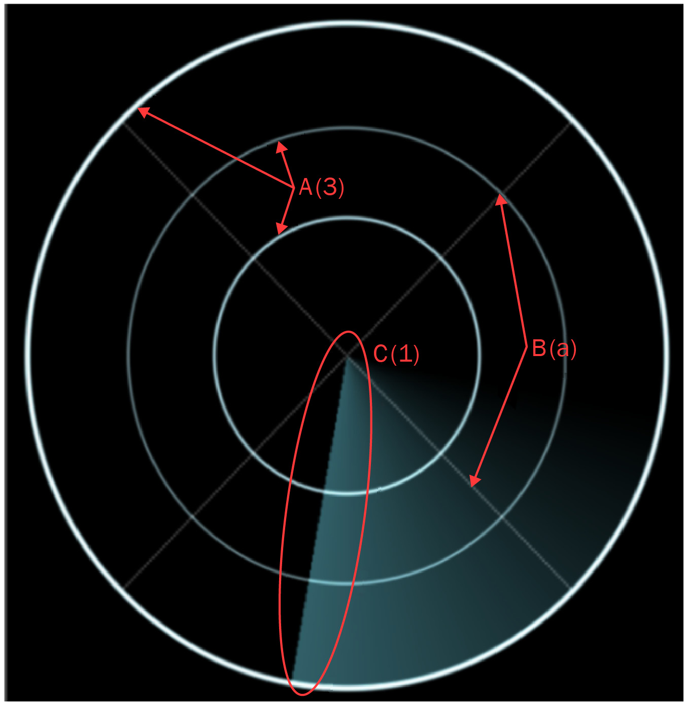
Figure 11.11 – The components of the Radar procedural texture

In the preceding diagram, the three circles (A), the two crossed lines (B), and the sweeping line (C) can each be examined independently of each other. Three concentric circles bind the texture, each a slightly different shade of light blue. Meeting at the center, each perpendicular to the other and oriented at 45 degrees concerning the upward direction are the crosses, in a darker blue-gray tone. Rounding out the static parts of the texture is the sweeping line, a turquoise-ish colored animated pizza slice with an opacity gradient. In the following screenshot, the node graph is shown fully collapsed down to its largest constituent components. Each element from Figure 11.12 has its own frame in the following screenshot:

Figure 11.12 – A node graph of the radar procedural texture

After grouping the major elements of the radar procedural texture, the node graph is still complex, but much easier to understand. Organizing and naming elements in the NME is important! For reference, the NME snippet can be found at #XB8WRJ#13.

To examine the specifics of any individual piece of the shader graph, expand the frame to see the steps comprising that portion of the fragment shader logic. The output of each frame varies a bit. Each CircleShape frame outputs a color value in the Add Circles frame, which, as its name implies, adds the color values together. A key element of procedural shape generation is that pixels that aren’t a part of the shape will be assigned a clear or empty color value. That’s why, if you peek inside the CircleShape, Cross, or Moving Line frames, you’ll find conditional nodes and other node operations that result in the output being set to a value between zero and one [0…1]. A value of 0 means the pixel isn’t a part of the shape at all. Any other value is indicative of the relative brightness of whatever the pixel’s final color ends up being.

The final color value is arrived at by individually scaling each element’s defined color (various shades of blue or white) by that brightness factor, then adding it together with the color output of all the other elements. Like magic, shapes emerge from a blank canvas! Regarding magic, one of the essential references mentioned at the beginning of this chapter was The Book of Shaders. The radar procedural texture was adapted from a ShaderToy example listed as part of its chapter on Shapes, located at https://thebookofshaders.com/07/. Even though there isn’t a node graph to be found on the site, every code snippet is interactive. Anyone interested in procedural textures or similar topics should make the time and effort to read through this concise, gentle, and amazingly well-put-together resource as part of continuing their journey in this area.

Very similar to Procedural Textures, the Post-Process mode of the NME works against the Fragment Shader. Let’s take a quick stroll through the landscape of Post-Processes in the NME.

Developing Post-Processes with the NME

Unlike the Procedural Texture mode, the Post-Process editor has a special Current Screen node. This node is an input texture that’s passed to the fragment shader. It contains a screenshot preview of the frame as it would be rendered without any post-processing. You can set any texture for this; its purpose is just to provide visual feedback on the post-process output.

One of the simplest Post-Processes that can be constructed with the NME is the never-out-of-style fade in/fade out mechanic:

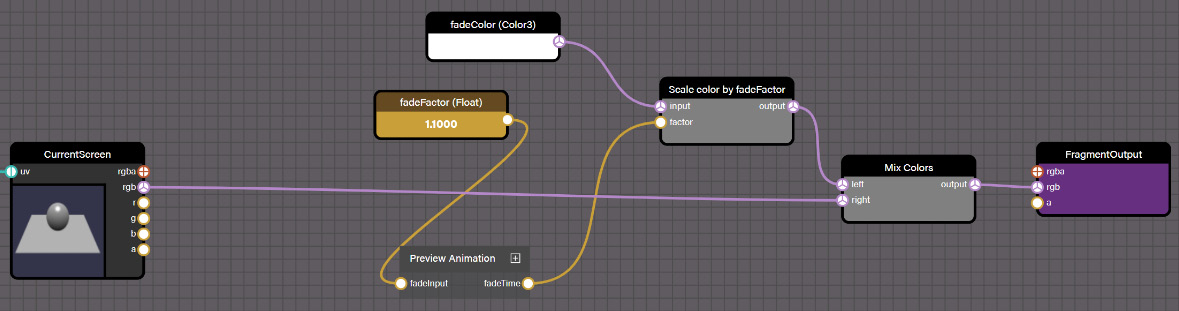
Figure 11.13 – Simple fade in/out post-process in the MNE

The Preview Animation frame is there to provide an animated view of what the post-process looks like in action. The fadeFactor uniform controls the degree of the effect. The snippet is hosted at Z4UNYG#2.

In the logic depicted in the preceding screenshot, the fadeColor node is scaled by a fadeFactor. To help visualize the effect, the Preview Animation frame passes the Time value through the Sin function to show the effect ping-pong between fadeFactors ranging from 0 (completely black) to 1 (normal) and up to 10 (completely white).

Important note

Because our scale starts at zero, assigning a value of 10 to fadeFactor is the same as cranking things up to 11, because that’s how far Babylon.js goes. You’ve been warned!

We started this section by learning about the basics of the NME and using our newly learned techniques to build a high-resolution Planet Earth Material, complete with animated cloud coverage. Because we took our time to go over the basics, we were able to pick up some steam heading into the topic of Procedural Textures. We learned that they are built very similarly to Materials, except the work is all done in the fragment shader. Like the Procedural Texture, Post-Processes do not operate against Scene geometry. A post-process is identical in function to a procedural texture because the Current Screen node is the rendered texture buffer for each pixel of the screen.

Summary

If it feels like we’ve been skirting a deep examination of this and the other topics we’ve covered so far in this chapter, then either you have a good sense of intuition or you read the title of this chapter. As this chapter’s title suggests, we’re only scratching the surface of a topic not only wide but deep in its complexity. That doesn’t mean that we haven’t covered a lot of material – quite the opposite! We started this chapter by learning a bit about some of the shader concepts and the differences between Vertex, Fragment, and Compute shaders. Each type of shader is a specialized software program that runs on the GPU once for every piece of geometry (vertex) and every pixel (fragment) on the screen.

None of the shader instances has any memory about things that happened in the previous frame and don’t know what any of their neighbors are doing. This makes shader programs a little bit mind-bending to work with initially. Fortunately, the language shader code used in Babylon.js is written in GLSL, which you should be familiar with if you are used to working with Python or JavaScript.

Compute shaders are new to Babylon.js v5.0 and are a powerful new addition to the WebGPU toolbox. Compute shaders are a more generalized form of a shader and unlike the vertex or fragment shader, they are capable of writing output to more than just a texture target or a mesh position. Therefore, they can perform parallel calculations of complicated systems such as fluid dynamics, weather, climate simulations, and many more things waiting to be invented.

Once we had a solid foundational understanding of shaders, we applied that knowledge to writing shader programs using the NME. The NME has several modes of operation, and we started again with the basics with the Material mode and the Planet Earth Material. After quickly learning how to add and mix textures, we topped the cake off with some icing by adding an animated effect to the cloud texture, learning about Frames as we went.

This knowledge of Frames came in handy when we tried to understand the much more complex Radar Procedural Texture. Ignoring the vertex output, the procedural texture and post-process modes operate against the fragment output. This similarity made it an easy transition to the Post-Process editor. Always classy and simple to implement, a basic fade in/fade out effect is quick to assimilate into our growing understanding of this important topic.

Like an iceberg’s tip peeking out of the water, there’s so much more to shaders and the NME than what’s visible from the surface. If this chapter were to do the topic its full justice, it would undoubtedly require another couple hundred pages! Be sure to check the next section, Extended Topics, for suggestions on where to go next and what to do.

We’ve come incredibly far along in our journey across the vastness of Babylon.js, but there’s still more ground to be covered. In the next chapter, we’re going to start moving from the express lanes over to the exit lane, but there are still a few more landmarks to make before we reach our destination terminal. In real-world terms, we’re going to shift our focus back to the overall application and learn about how to make Space-Truckers run offline and record high scores before publishing it to a major app store. If that sounds like a refreshing change of scenery, then read on! Otherwise, if you’re looking for some side-quests to keep things going in the Land of Shaders, the Extended Topics section might have some interesting challenges you can undertake. See you in the next chapter!

Extended Topics

Here are some ideas on ways to further your journey with the NME in particular, but also some resources on shaders in general:

• Use the techniques we learned about in this chapter to create procedural clouds for the Planet Earth Material. One way to approach this would be to start with the existing cloud texture and distort it using some type of Noise node.
• The Book of Shaders (https://thebookofshaders.com/) is a free online resource that, while still an evolving work-in-progress, can be, as the authors describe it, “a gentle step-by-step guide through the abstract and complex universe of Fragment shaders.” Even though it focuses entirely on Fragment shaders, it is nonetheless a spring-powered steppingstone toward improving your understanding of shaders. Each chapter introduces examples and exercises along with the necessary material – try reproducing examples from this book in the NME. Post your results on the BJS forums and see what others have done at https://forum.babylonjs.com/c/demos/9.
• It can be tough to understand what’s going on in the GPU, especially since there’s no easy way to attach a debugger and step through code like many might be used to doing with regular code. SpectorJS is a browser extension that can give insights into what is happening on the GPU. You can learn more at https://spector.babylonjs.com/.
• The TrailMesh that extrudes along the route taken by the simulated cargo passes through different encounter zones on its journey. Create a Node Material or Texture that takes in encounter zone information and uses it to render the trail mesh in a unique pattern for every zone.
• Related to the preceding bullet point, create an effect that is triggered whenever an encounter is rolled during route planning. The effect should be positioned at the location of the encounter and can be different according to the type of encounter (although it needn’t be). For gameplay purposes, it probably shouldn’t reveal too much information to the player, but it can certainly tease!
• The Babylon.js Docs contain numerous topics and resources about the NME. They also contain links to various YouTube videos that provide tutorials on different aspects of using the NME:
  • Creating and using Node Materials in code. If you are writing a paper or a book about programming and want to sound smart, “Imperatively Reflecting JavaScript into GLSL” is a good title: https://doc.babylonjs.com/divingDeeper/materials/node_material/nodeMaterial.
  • A list of related videos can be found at the bottom of the preceding link. Video topics include PBR Nodes, Procedural Projection Textures, Procedural Node Materials, Anisotropy, and more!