8

Building the Driving Game

It may not be easy to believe it, but we are officially past the halfway point – while the end is still not in sight, we’ve made so much progress it’s tough to see our starting point. In the previous six chapters, we built out a huge amount of functionality encompassing an almost breathtaking diversity of subjects. The following figure shows where we were before and where we are now:

Figure 8.1 – How it started versus how it’s going. A montage of screenshots showing our progress

From setting up the basic web application to implementing random encounters, a lot has gone into our code base to get to this point, but we’re not stopping or even slowing down any time soon! Making it this far into this book shows admirable persistence and determination – this chapter is where all of that will pay off. One of the more enjoyable aspects of game development is also one of the more obvious ones – the part of getting to work on the core gameplay and logic code. Unfortunately, and as people with experience of developing and shipping software will attest, all the other activities that go into building and delivering software tend to take up the lion’s share of available project time.

Throughout this chapter, we’re going to be building out the driving phase of Space-Truckers. Along with some of the techniques we learned earlier, we’re going to introduce a few new tools for the ol’ toolbox. We’re going to take things up a notch by adding a second camera to our scene that will render the Graphical User Interface (GUI). We’ll generate a route based on the previous phase’s simulated route and allow players to drive their trucks along it, avoiding obstacles (if they can). Our scene will use physics as the previous phase does, but instead of mainly using it as a gravitational simulation, we’re going to make use of the physics engine’s capabilities to simulate the results of collisions, friction, and more. Some things we’re going to introduce but defer more detailed examination until upcoming chapters – when this is the case, the relevant chapters and sections will be linked for easy reference.

All those exciting topics will hopefully more than make up for the more mundane but no less important task of building the necessary logic ahead of us. By the end of this chapter, we’ll have a playable driving game that sets us up for the following chapter, where we will continue to finish the overall game’s life cycle as we learn how to calculate and display scoring results.

In this chapter, we will cover the following topics:

• Prototyping the Driving Phase
• Integrating with the Application
• Adding Encounters
• Making the Mini-Map

Technical Requirements

Nothing in this chapter is required from a technical perspective that hasn’t already been listed as being needed for the previous chapters, but there are some technical areas where it might be useful to have working knowledge as you read through this chapter:

• MultiViews: https://doc.babylonjs.com/divingDeeper/cameras/multiViewsPart2
• Layer Masks: https://doc.babylonjs.com/divingDeeper/cameras/layerMasksAndMultiCam
• In-Depth Layer Masks: https://doc.babylonjs.com/divingDeeper/scene/layermask
• Loading Any File Type: https://doc.babylonjs.com/divingDeeper/importers/loadingFileTypes
• Polar Coordinates: https://tutorial.math.lamar.edu/Classes/CalcII/PolarCoordinates.aspx and https://math.etsu.edu/multicalc/prealpha/Chap3/Chap3-2/

Prototyping the Driving Phase

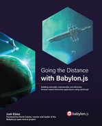
There’s a lot to do, so let’s dive right into it. Due to the way the driving phase is designed, players must navigate their trucks along a route that’s been pre-determined by the players in the previous game phase. The nature of the overall planned route determines similar overall characteristics of the driving route. Factors such as total transit time, distance, and velocities all fall into that kind of characteristic. Others, such as random encounters along the path, are more localized to a specific portion of the path. The behavior of each encounter is variable, but all will have a general form of forcing the player to make choices to avoid/obtain a collision while piloting their space-truck. Capturing the correlations between the two phases is an important design specification that will be useful – here’s what is listed on the Space-Trucker Issue created for that purpose:

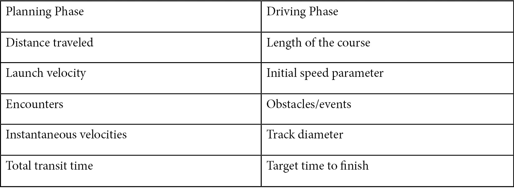
Figure 8.2 – Comparison of Route Planning versus driving phase variables. Source: https://github.com/jelster/space-truckers/issues/84

Some of the properties have a direct 1:1 correlation between phases, such as total transit time and distance traveled. Others are used as scale or other indirect influencing factors, such as the point velocity affecting the route’s diameter. This will all be quite useful a bit further down this chapter’s journey, but for now, we will turn our attention to building out a Playground demonstrating the core principles of the driving phase.

Playground Overview

Prototyping in software is all about reducing a particular problem or area of interest to its bare essence. It forces us to ask the question – what is the smallest set of characteristics, attributes, features, and so on needed to evaluate the viability of a particular approach? In the case of our driving phase prototype, we don’t need to play through the planning phase to accomplish our goals – we just need to be able to process the route data generated by that phase. Focusing in, the problem of hooking up our route data to the driving phase isn’t the problem we’re trying to solve right now (though we can certainly do our future selves a solid by structuring our code in ways that facilitate building that logic!). This saves mental bandwidth and energy that can be put to good use elsewhere, which is where we will begin.

Important note

The Playground at https://playground.babylonjs.com/#WU7235#49 is the reference for this section of this chapter.

We’ll need physics to be working so that we can playtest the interactions and relationships between the truck, obstacles, and velocities. We need to determine the proper scaling, orientation, and import settings for loading the first 3D asset model into the game – the semi-truck. Finally, we need to figure out how we’re going to plot oncoming obstacles in the radar GUI presented to the player. This seems like quite a lot to take on, but thanks to the functionality built into Babylon.js there’s much less complexity than it might seem. The following screenshot illustrates how these elements all come together in the Playground demo:

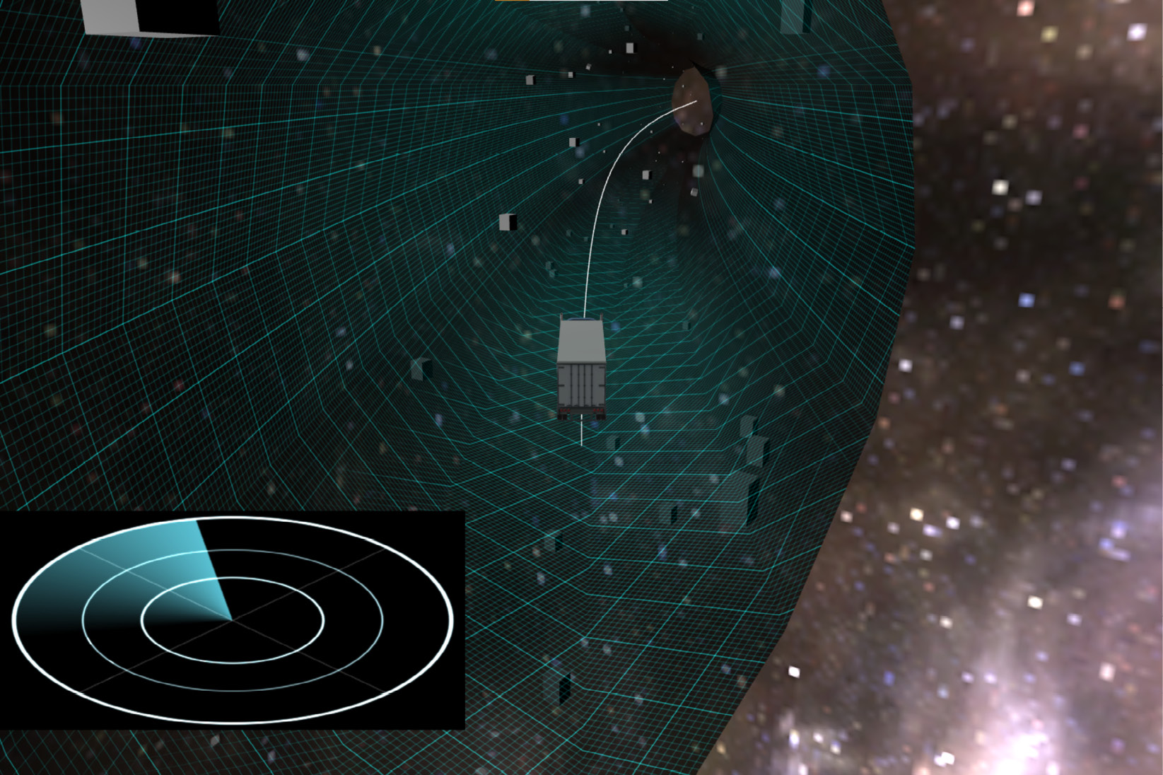
Figure 8.3 – Space-Truckers driving phase Playground at https://playground.babylonjs.com/#WU7235#49

In the center of the viewport is our game’s protagonist, the eponymous space-trucker. The space-road stretches out in front of them, littered with the untextured blocks that are filling the place of encounters. In the lower-left part of the screen, a radar display sweeps in a circle, revealing upcoming obstacles as blips. The camera is chained to the truck so that the player’s perspective is always behind and a bit above the truck – the classic Third-Person Perspective. The controls are simple – W and S accelerate and decelerate in the truck’s forward direction, while A and D accelerate to the left and right, respectively. Vertical acceleration is managed with the up arrow and down arrow keys, and rotation with the right arrow and left arrow; resetting the demo is done by pressing the Delete key. Try to make it to the end of the path as fast as you can!

Let’s swap over to looking at the code for the demo, and how the demo is structured. Right away, we can see some similarities but also some differences from how we’ve structured our previous Playground demos. At the very top are the various asset URL and BABYLON namespace aliases; moving down, we have a rather hefty gameData object, and then we get to the most striking difference yet: the async drive(scene) function.

This is, as implied by the async prefix, an asynchronous JavaScript function. Its purpose is two-fold: one, to allow the use of the await statement in expressions within the function body, and two, to provide a container for closure over all the *var*-ious objects and values used by the demo.

Note

The editors of this book apologize for subjecting you to the inredibad pun that was just made.

Furious punning discharged, we will continue with the first few lines of the PG above the drive function. To load our route data, we’ll choose the simple approach of wrapping a call to jQuery.getJSON in a promise that resolves to the array of route path points:

var scriptLoaded = new Promise(
    (resolve, reject) =>
        $.getJSON(routeDataURL)
            .done(d => resolve(d))
);

This requires us to specify our createScene method as async, allowing us to write a simple harness to instantiate and return the Playground’s Scene after doing the same for the driving phase initialization logic:

var createScene = async function () {
    var routeJSON = await scriptLoaded;
    var scene = new BABYLON.Scene(engine);
    const run = await drive(scene, routeJSON);
    run();
    return scene;
};

The drive function is responsible for creating and/or loading any type of asset or resource that might require a bit of time to complete, so it is also marked as async. There’s a ton of code that goes into this function, so to make it easier to work with, the logic is split up into a few helper methods. Before those, the logic for basic scene and environment setup is constructed or defined. These are elements that might be needed by any or all the (potentially asynchronous) helper functions that include the invocation of those helper functions in the proper order. Once those tasks are complete, the run function is returned:

await loadAssets();
initializeDrivingPhase();
initializeGui();
return run;

We’ll cover the initializeGui method in this chapter’s Making a Mini-Map section after we establish a bit more context. Earlier in the drive function is probably the most important helper function that we want to prove out in the Playground, and that is the calculateRouteParameters(routeData) method. This is the workhorse function of the driving phase’s world creation and has probably the largest impact on how gameplay evolves in the form of dictating the properties of the route driven by the player.

Generating the Driving Path

In Chapter 7, Processing Route Data, we set up cargoUnit to log routeData: timing, position, velocity, rotation, and gravity are all captured every few frames of rendering into a collection of data points (along with encounters, which we’ll get to in the Adding Encounters section). The telemetry data is a deep well for creative and interesting ideas (see Extended Topics), but for now, we’ll just use the position, velocity, and gravity route values described in the Playground Overview section to generate the route path.

The beginning of the function grabs routeDataScalingFactor from gameData; though currently set to a value of 1.0, changing this allows us to scale the route size and length consistently, easily, and quickly across route elements. In a concession to our desire to load up captured route telemetry from a JSON file, we iterate through the data array to ensure that the position, gravity, and velocity elements have been instantiated to their respective Vector3 values, as opposed to a Plain Ol’ JavaScript Object.

Important note

Taking proactive steps like this to reduce friction on quick iteration is key to building momentum!

Once that’s done, we use the positional vectors from the telemetry data to construct a new Path3D instance:

let path3d = new Path3D(pathPoints.map(p => p.position),
  new Vector3(0, 1, 0), false, false);
let curve = path3d.getCurve();

From the Babylon.js docs (https://doc.babylonjs.com/divingDeeper/mesh/path3D),

“A Path3D is a mathematical object created from a sequence of position vectors of points on a curve.”

Error! Hyperlink reference not valid.

Put another way, a Path3D represents an ordered set of coordinate points with some interesting and useful properties.

Note

The reason for calling it a “mathematical object” is because it is not a member of the Scene and does not take part in rendering. This also sounds a lot cooler than calling it a “non-rendered abstract geometrical data structure.”

The getCurve() method is a utility method that spits back the sequence of points that define the path, but there are even more useful nuggets of value tucked away in Path3D that we’ll soon be exploring. First, though, we want to display the specific path taken by the player during the planning phase as a straight line going down the middle of the space-road. This is easy – we use the curve array in a call to MeshBuilder.CreateLines and that’s all there is to it! For more on this, see https://doc.babylonjs.com/divingDeeper/mesh/creation/param/lines. After that is when we start constructing the geometry for the space-road, which is where things start to get interesting.

The geometric shape forming the base of our space-road is a Ribbon – a series of one or more paths, each with at least two Vector3 points. The order the paths are provided works in conjunction with the paths themselves to produce geometry with a huge range of flexibility, and though potentially entertaining, it would be counterproductive to attempt to reproduce the excellent examples already created as part of the Ribbon’s documentation at https://doc.babylonjs.com/divingDeeper/mesh/creation/param/ribbon_extra. From those docs, this thought experiment nicely explains the concept we’re looking at currently:

“Imagine a long ribbon of narrow width in the real world with a wire running down its length. Closing the paths forms a loop of ribbon while closing the array would form a tube.”

Closing the array seems like the option we want rather than closing the paths themselves since we want our road to be enclosed, but not like a donut or loop. This faces us with a bit of a choice regarding how we’d like to approach implementing this, but only after we have established the value in doing it via prototyping, which in this circumstance becomes the link back to our choice of implementation paths in an endlessly circular argument.

When prototyping out the path creation (or any prototyping process in software), there’s a certain point in the process where you realize the need to transition from throwing something together to see if it works and taking consideration to build something more robust with the knowledge that it will be incorporated into the final product. Playground snippet #WU7235#11 (https://playground.babylonjs.com/#WU7235#11) shows, starting around line 168, what this prototyped logic can look like (comments have been removed for clarity):

let pathA = [];
let pathB = [];
let pathC = [];
let pathD = [];
for (let i = 0; i < pathPoints.length; i++) {
    const { position, gravity, velocity } = pathPoints[i];
    let p = position;
    let speed = velocity.length();
    let pA = new Vector3(p.x+speed, p.y-speed, p.z+speed);
    let pB = new Vector3(p.x-speed, p.y-speed, p.z-speed);
    let pC = pB.clone().addInPlaceFromFloats(0, speed * 2,
      0);
    let pD = pA.clone().addInPlaceFromFloats(0, speed * 2,
      0);
    pathA.push(pA);
    pathB.push(pB);
    pathC.push(pC);
    pathD.push(pD);
}

This is a scheme for path geometry that takes the form of a four-sided box (the ends are open). The preceding code uses four separate arrays of points – one for each corner – to capture the paths as it loops through each of the points along the route. This is what that looks like:

Figure 8.4 – Prototype path geometry hardcoded to make a four-sided box with open ends. Four paths are used. Simple and effective, yet extremely limited (https://playground.babylonjs.com/#WU7235#11)

Mission accomplished! We’re done here, right? Wrong. This is just the beginning! It’s OK to celebrate accomplishments, but it’s best to keep any celebrations proportional to the achievement in the context of the end goal. A box shape works to prove that we can create a playable path demo from actual route data, but it’s not particularly fun or attractive to look at. To step this up to a place where it’s something that will surprise and delight users, we need to make it more spherical and less boxy. We need to add more path segments to do this, and that’s where our prototype reaches its limits.

Referring to the previous code listing, each path of the ribbon has been predefined in the form of the pathA, pathB, pathC, and pathD arrays. If we want to add more segments, we need to manually add the additional path array, along with the appropriate logic, to locate path segments that aren’t at 90-degree right-angles to each other correctly – and that makes our current approach much tougher. There’s a certain mindset that prefers to attack this sort of problem head-on, with brute force. They might add pathE, pathF, or pathG arrays and pre-calculate the paths’ offsets relative to one another based on hardcoded numbers and after the dust settles, what comes out will probably work just fine… until the need arises to change the number of segments again. Or worse yet, the need arises to dynamically set the number of paths based on, for example, device performance characteristics. That’s why it’s necessary to come up with a Better Way Forward.

Let’s jump back to the original Playground we started with – #WU7235#23 – and look at how it’s evolved starting at line 140. First things first, we know that we need to be able to specify how many separate paths should be created. That’s easy – just define a NUM_SEGMENTS constant. Next, we need to instantiate new path arrays to hold each path. We do this in a simple loop:

const NUM_SEGMENTS = 24;
let paths = [];
for (let i = 0; i < NUM_SEGMENTS; i++) {
    paths.push([]);
}

Great – we have our array of path arrays ready to go. Now, it’s time to populate those paths, so we set up an outer loop over routePath containing an inner loop over each path array. But how do we figure out where each point of each path is supposed to be located? It’s not enough to use the simple constant offsets to each point position like we did in the prototype; each path segment’s points will have different offset values from each other. In the following diagram, the hoop or ring shape is a single cross-section segment, with all points lying in the same plane (math folks call this an affine set of points):

Figure 8.5 – Creating a point of route geometry starts from the center point that moves clockwise around the diameter, adding path points for each discrete segment

Start from the current route position and use it as the center point. Now, focusing on one individual execution of the outer-most loop through routeData, we know that we need to create points equal in number to the number of desired segments. We also know that those segments should be evenly and contiguously distributed around the diameter of a hypothetical circle.

Note

The reason we use a circle rather than a sphere is that relative to a given route point, the Z-axis values will always be the same for every path segment around that point. This is rather tautological since that’s also a somewhat meandering way to define a circle!

Putting those facts together and combining them with what we already know regarding circles and trig functions, we have a way to do just what we want. There’s just one remaining obstacle: how can we vary the position offset on the individual path being computed? Fortunately, this isn’t as big of an issue as it might seem at first.

Let’s remind ourselves of these facts about circles and trigonometric functions. The sine and cosine functions each take an input angle (in radians for this text unless otherwise noted) and output a value between -1 and 1 corresponding to the angle-dependent X- and Y-axis values, respectively. A full circle comprises two times Pi (3.14159…) radians, or about 6.28 radians. If we divide the number of segments by 6.28 radians, we would get the arc that an individual segment traverses, but if we divide the number of segments by the zero-based index of the currently iterating segment, then we get something more useful – the position between 0..1 of our current segment. A percentage, or ratio in other words. By multiplying that ratio with our two times Pi value, we get… the position of the segment, in radians! All that’s left is to scale the result by a value representing the desired radius (or diameter, for the X-axis) and add it to the path collection:

for (let i = 0; i < pathPoints.length; i++) {
    let { position, velocity } = pathPoints[i];
    const last = position;
    for (let pathIdx = 0; pathIdx < NUM_SEGMENTS;
      pathIdx++) {
        let radiix = (pathIdx / NUM_SEGMENTS) *
          Scalar.TwoPi;
        let speed = velocity.length();
        let path = paths[pathIdx];
        let pathPoint = last.clone().addInPlaceFromFloats(
            Math.sin(radiix) * speed * 2,
            Math.cos(radiix) * speed, 0);
        path.push(pathPoint);
    }
}

In the preceding code listing from #WU7235#25, we are using the length of the point’s velocity vector to determine the size of the space-road. We must clone the last point before mutating it; otherwise, we will end up corrupting the data needed by the rest of the application. By setting the value of NUM_SEGMENTS to 4 and progressively running the Playground at increasing numbers, it’s easy to see that the updated logic can now handle an arbitrary amount of line segments – an enormous improvement over our first-generation prototype! This code will be ready to integrate with the application when we’re ready to begin that process starting in the Initializing the Driving Phase section. There are still a few more things to prove out in other areas before that can happen, though. The loadAssets function is next up on our list.

Loading Assets Asynchronously

In this Playground, we’re going to be loading two things asynchronously as part of the loadAssets function – the semi-truck model and the radar procedural texture asset. We need to make sure that all the asynchronous function calls have been completed before continuing by returning a promise that resolves only when all of its constituent promises have done so as well. Here’s what that looks like in loadAssets():

return Promise.all([nodeMatProm, truckLoadProm])
          .then(v => console.log('finished loading
            assets'));

nodeMatProm is created using a pattern that is used throughout Babylon.js and one we most recently used in the previous chapter’s discussion on loading JSON for a ParticleSystemSet, only for this Playground, instead of loading JSON directly, we will load data from the Babylon.js Snippet Server. Specifically, we are loading a snippet from the Node Material Editor (NME) that we will then use to create the radar procedural texture that is displayed on the GUI. Further details on those elements will have to wait until Chapter 11, Scratching the Surface of Shaders:

const nodeMatProm = NodeMaterial.ParseFromSnippetAsync
  (radarNodeMatSnippet, scene)
      .then(nodeMat => {
         radarTexture = nodeMat.createProceduralTexture(
         radarTextureResolution, scene);
      });

While it may be obvious that radarTexture is a variable containing the procedural texture, it’s less obvious where the radarTextureResolution value comes in. One of the difficulties in creating a “simple” game prototype is that even something simple requires creating and managing a fair amount of configuration data. The gameData structure serves the purpose of centralizing and consolidating access to these types of values; when we want to utilize one or more of these values in a function, we can use JavaScript’s deconstruction feature to simplify and make our code much more readable:

const { 
        truckModelName, 
        truckModelScaling, 
        radarTextureResolution } = gameData;

As we saw in the preceding code block, radarTextureResolution is used for determining the render height and width in pixels of the procedural texture, whereas we’ll shortly see how truckModelName and truckModelScaling are used. The SceneLoader.ImportMeshAsync method (new to v5!) takes an optional list of model names, along with the path and filename of an appropriate file containing the meshes to load (for example, .glb, .gltf, .obj, and so on), along with the current scene. The promise that’s returned resolves to an object containing the loaded file’s meshes, particleSystems, skeletons, and animationGroups, although we’re only going to be using the meshes collection for this scenario.

Note

You can learn more about SceneLoader and its related functionality at https://doc.babylonjs.com/divingDeeper/importers/loadingFileTypes#sceneloaderimportmesh.

Once we’ve loaded the semi-truck’s model file, we’ve got a bit more work to do before we can start using the loaded asset. Models saved in the GLTF or GLB formats are imported into Babylon.js with some additional properties that are going to get in our way, so let’s simplify and set up truckModel for the game world:

const truckLoadProm = SceneLoader.ImportMeshAsync
  (truckModelName, truckModelURL, "", scene)
    .then((result) => {
        let { meshes } = result;
        let m = meshes[1];
        truckModel = m;
        truckModel.setParent(null);
        meshes[0].dispose();
        truckModel.layerMask = SCENE_MASK;
        truckModel.rotation = Vector3.Zero();
        truckModel.position = Vector3.Zero();
        truckModel.scaling.setAll(truckModelScaling);
        truckModel.bakeCurrentTransformIntoVertices();
        m.refreshBoundingInfo();
    }).catch(msg => console.log(msg));

The first few lines of our processing pipeline perform some convenient setup for the variables from the result structure, but then we do something a bit unusual by setting the parent of truckModel to null before disposing of the first mesh in the meshes array – what’s up with that, and what’s with SCENE_MASK?

Note

For more on layer masks and how they operate, see the docs at https://doc.babylonjs.com/divingDeeper/cameras/layerMasksAndMultiCam.

The answer to the second is, briefly, that cameras can be assigned a specific number that only allows meshes with a compatible layerMask to be rendered by that camera. We use the layerMask property to hide non-GUI meshes from the main scene camera, for example. The answer to the first lies in the specifics of how an asset is loaded from a GLB or GLTF file. When Babylon.js reads in the file, there is an invisible transform node named __root__ placed at the root of the model hierarchy. Although it doesn’t cause any problems in simple scenarios, when dealing with physics, parenting, collisions, and transforms, it becomes a major hindrance. The following screenshot illustrates what this looks like in the Scene Inspector window:

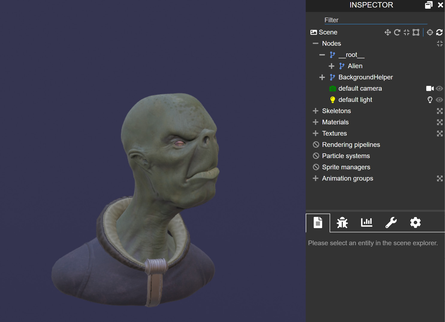
Figure 8.6 – The Alien.gltf model. The Scene Inspector window shows the __root__ transform node. From https://playground.babylonjs.com/#8IMNBM#1

The Alien geometry is what we’re interested in working with, but because it is parented to the __root__ node, any changes to the position, rotation, or scaling of Alien are evaluated in a coordinate space relative to that root node, resulting in undesired and unpredictable results. The solution to this is simple and answers our earlier question regarding what was up with our loadAssets code – unparent the desired mesh and dispose of the root. Once that’s accomplished, the rest of the code in our truck loading method is all housekeeping setup for the model – with some important considerations to keep in mind:

• Order of operations is important, but not in the way you might think. Changes to a TransformNode (which Mesh is a descendent of) over a given frame are applied in the fixed order of Transform, Rotate, Scale (TRS).
• Use setParent(null) rather than the alternative of setting mesh.parent = null. The setParent function preserves positional and rotational values, whereas setting the parent to null does not. This results in any root transformations being removed from the mesh, which is why we need to reset the position and rotation vectors.
• Once the transformations have been cleared and the scaling has been set to world-appropriate values, the mesh geometry will need to have new bounding information generated. Otherwise, collisions won’t work properly. The solution to this is the two-step process of calling mesh.bakeCurrentTransformIntoVertices() before calling mesh.refreshBoundingInfo().

Important note

Normally, it’s not recommended to call bakeCurrentTransformIntoVertices when there are better options such as parenting and pivotPoints that might work. In this case, we need to perform this step since we’ve removed the parenting to root. See https://doc.babylonjs.com/divingDeeper/mesh/transforms/center_origin/bakingTransforms for more information and guidance on this topic.

As mentioned previously, the result of calling Promise.all with the unresolved promises is the returned Promise from loadAssets, bringing us full circle back to where this discussion started! Initialization is mostly done – or at least the portion of it taking the longest time is complete – and now with the availability of the semi-truck model, the initializeDrivingPhase function has been invoked to set up the rest of the scene’s elements. This function sets up the cameras, creates the ground ribbon mesh from the routePaths, sets up physics, and more.

Initializing the Driving Phase Scene

As mentioned in this chapter’s introduction, the viewpoint for the player is in a third-person perspective, with the camera behind the semi-truck and looking over its top. As the truck moves (translation) or rotates (um, rotation), the camera mimics every movement from its offset position. The way this is accomplished is one of those situations where real-world analogies match well to software, in the form of cameraDolly.

A camera dolly is normally an engineered sort of cart used in the film industry that allows the Grip operating the camera to smoothly move in multiple dimensions while capturing footage. Our camera dolly doesn’t run on tracks, but it fulfills a similar purpose by moving with the truck to maintain the same forward-facing orientation regardless of the truck’s world-space orientation. This can be accomplished in just a few steps:

1. Create a TransformNode to serve as the “camera dolly:”

   var cameraDolly = new TransformNode("dolly", scene);
2. Define an ArcRotateCamera and set up its basic properties. We’re patching property values in from gameData structures to reduce the amount of code:

   for (var k in followCamSetup) {

       followCamera[k] = followCamSetup[k];

   }
3. Order of operations is important for this and the next step! First, parent cameraDolly to truckMesh.
4. Now, parent followCamera to cameraDolly:

           cameraDolly.parent = truckModel;

           followCamera.parent = cameraDolly;

The first thing that happens in the initializeDrivingPhase method is that the camera gets created and the Viewport is set up. A quick aside to explain a bit more about that.

If a Camera is a bridge between a Scene and the Display, then a Viewport is what defines the Display aspect of that bridge. The default Viewport is fixed at coordinates (0,0) and has a size of (1,1). In other words, the default Viewport’s top-left corner is located at (0,0) and the bottom-right corner is located at (1,1); the entire screen is covered by it. This is greatly desired when a Scene has but a single camera, but there are many circumstances where it is useful to have a second camera positioned somewhere in the scene that renders to a smaller segment of the full screen – think of strategy games that provide a mini-map or racing games that have a rear-view mirror display.

In most cases, there are elements of the scene that should be rendered just in one camera, but not in another, which is finally where we make the connection with Layer Masks. By setting layerMask of all the involved cameras and meshes, we can efficiently show or hide geometry according to the mesh’s role in the scene. Our driving screen currently has two separate layer masks: SCENE_MASK and GUI_MASK. Cleverly toggling a mesh’s layerMask property can allow fine-grained control over camera rendering; if we want to display the mesh on one camera or the other, we can explicitly set its layerMask to SCENE_MASK or GUI_MASK (0x00000001 and 0x00000002, respectively). If we wish to display a mesh on both cameras, we can set and/or leave the default layer mask value in place (0xFFFFFFFF). Now that we know what’s going on with the viewport, we can get back to the function code.

After setting up the viewport, the parenting steps listed previously are executed. The MeshBuilder.CreateRibbon method is the next point of interest, where we pass the array or path arrays into the options of the function and get back our path geometry, which then gets some property tweaks and a grid material (for now) assigned:

var groundMat = new GridMaterial("roadMat", scene);
var ground = MeshBuilder.CreateRibbon("road", {
    pathArray: route.paths,
    sideOrientation: Mesh.DOUBLESIDE
}, scene);
ground.layerMask = SCENE_MASK;
ground.material = groundMat;
ground.visibility = 0.67;
ground.physicsImpostor = new PhysicsImpostor(ground,
    PhysicsImpostor.MeshImpostor,
    {
        mass: 0,
        restitution: 0.25
    }, scene);

With the ribbon created, material assigned, and a physics impostor similarly created and assigned to the ground mesh, the restitution property makes anything hitting the wall rebound with a little less momentum than before. That’s new, but there’s a bit of a twist (highlighted in the preceding code block) with the type of impostor we’re using here as well – MeshImpostor. Previously only available in the CannonJS physics plugin, where it is limited to interacting only with spheres, MeshImpostor is different from the other PhysicsImpostor types we’ve previously looked at (Box and Sphere).

Instead of using a rough approximation of the physics-enabled object’s geometry, it uses that very geometry itself to provide precise collision detection! The trade-off is that collision computation becomes more expensive the more complex the mesh’s geometry is structured. We should be OK for our needs though, since we don’t need our obstacles (that is, encounters) to interact with the path, leaving just the truck with complex collision calculation needs. Just a few more tasks remain before we will be done with our preparations and be ready to write the runtime logic!

After setting up the physics of truckModel – albeit using the equally applicable and much simpler BoxImpostor – we spawn some sample obstacles along the path before setting up an OnIntersectionExitTrigger that calls killTruck whenever the truck exits the routePath ribbon mesh’s confines. The spawnObstacles function will ultimately be discussed in the Adding Encounters section, so skipping over a discussion of that leads us to the familiar-in-practice of setting up ground.actionManager with the appropriate trigger (see the section on Defining the EncounterZones in Chapter 7, Processing Route Data) – another place that is familiar enough to skip past. Now, we approach the final act of the initializeDrivingPhase function – (re)setting the truck to its starting position and state.

Using our sample route data, we could empirically determine what coordinates in the world space the truck should start at, its initial rotation, and other such values. We would iteratively refine our values through trial and error until the results were satisfactory, but would that satisfy our requirements? No.

Note

If you ever see a question asked in the preceding fashion, the answer is almost always “No.” This is the second instance in this chapter of that kind of rhetorical writing. Can you spot the third?

That entire trial and error approach will not “satisfy our requirements,” no thank you sir! We can make this extremely easy on ourselves by recalling that we already know exactly and precisely where the truck should start, where it should be pointing, and how fast it should be moving in the form of our pal route.path3d. It was mentioned in the earlier discussion on Path3D, it is a mathematical construct, and two of the more useful functions it provides, getPointAt and getTangentAt, are used to help us position the truck, but we didn’t get much into the details of why they’re useful.

Think about a path of some arbitrary length that consists of several points. Every point along that path has a set of vectors describing the position (naturally!), the tangent (a vector pointing in the direction of travel at that specific point along the curve), the normal (an arbitrarily chosen vector pointing perpendicularly to the tangent), and the binormal (a vector chosen to be perpendicular to the normal). These are all computed for us by the Path3D instance, making it easy to work with.

If we think of the point’s position in the path’s collection of points (that is, what index it occupies in the array) as being the ratio between the index and the total number of elements, then we can easily picture that ratio being a percentage, or a number between 0 and 1 (inclusive of both). Interpolated functions of the Path3D module all accept a number representing the percentage (between 0 and 1) along the path to operate against and include the related getNormalAt, getBinormalAt, and getDistanceAt functions.

Note

There are more interpolation functions to explore! See https://doc.babylonjs.com/divingDeeper/mesh/path3D#interpolatio for the full list.

This is useful because you don’t need to know what the length of the path is or how many points are in it to obtain useful information. In the resetTruck function, we get the position and the tangent of the first point in the route – the beginning of the path – then set the truck’s properties accordingly:

const curve = route.path3d.getPointAt(0);
const curveTan = route.path3d.getTangentAt(0);
truckModel.position.copyFrom(curve);
truckModel.rotationQuaternion =
  Quaternion.FromLookDirectionRH(curveTan, truckModel.up);
truckModel.physicsImpostor.setAngularVelocity(currAngVel);
truckModel.physicsImpostor.setLinearVelocity(currVelocity);

Since the physics engine sets and uses the rotationQuaternion property, we can’t just use the vector provided by getTangentAt(0) – we need to convert it into a Quaternion using the FromLookDirectionRH method. This function takes two vectors for its arguments: the first, a vector representing the desired forward direction, and then another vector representing the orthogonal (for example, perpendicular along all axis), with the return value being a Quaternion representing the input vectors. After setting the truck’s position and rotation, it’s necessary to reset the truck’s physical values for velocity since, from the physics engine’s perspective, the effects of being moved and rotated would need to be considered. Therefore, the reset method is a deterministic function – the effect on the state of the scene is always the same whenever it is called. This makes it especially useful to use it both immediately post-initialization and any time that the player chooses to do so. We listen for that player input in this Playground’s update method.

Running the Update Loop

Most of the code discussed up to this point has been code that directly relates to the context at hand. That’s the great thing about Babylon.js and its tooling – many common tasks are possible to complete with just a few lines of code. The update method is a good example of that but it’s also an example of one of the few places in the Playground where the code will need to be changed around completely to integrate it with the application, simply due to the more complex nature of the application versus the much more narrowly scoped Playground (see the next section, Integrating with the Application, for more). For that reason, we aren’t going to look too hard at the specifics of the function and instead focus on the mechanics of how the truck is controlled by the logic in it.

The truck can be controlled in the three translational axes (forward/back, left/right, up/down) and one rotational axis (the yaw axis), which might seem to make for a total of eight separate pieces of logic to handle the motion. However, since pairs of actions (for example, left and right) are simply the negated values of each other, we only need to figure it out for four – a nice reduction in complexity. In each frame, the delta frame time variable is used to scale truckAcceleration and truckTurnSpeedRadians to the correct values; the currVelocity and currAngVel counter variables track the accumulated changes that are then applied to the physics model’s linear and angular velocities at the end of the update process. This is like what we’ve done in the past, but some mathematical tools are being employed that we’ve not yet seen that are worth taking a closer look at.

Changing the forward or backward translational velocity is simple – just get the current forward vector for the truck mesh, scale it by currAccel, then add it to the currVelocity counter; the backward vector consists of the negated value of the forward vector:

if (keyMap['KeyW']) {
    currVelocity.addInPlace(currDir.scale(currAccel));
}
else if (keyMap['KeyS']) {
    currVelocity.addInPlace(currDir.scale(currAccel)
        .negateInPlace());
}

All of the various Vector3 math methods come in various flavors that allow the developer to control whether or not the operation should allocate memory or reuse an existing object. In this case, we are using the addInPlace function to avoid creating a new vector object, whereas we create a new Vector3 with the currDir.scale(currAccel) function call to avoid corrupting the truck mesh’s forward vector – a value relied upon by the engine for proper rendering.

Important note

Knowing when and what to perform memory allocation and disposal with can be key to a smoothly rendered scene. See Chapter 13, Converting the Application to a PWA, for more information and guidance.

Back to our truck’s control logic, the mathematical trick is in how we figure out what direction to apply the remaining translational and rotational forces. Translating to the truck’s left or right is done by taking the cross product of the truck’s forward vector and the truck’s up vector – the result is a vector pointing in either the left or right direction (the same trick with negateInPlace can yield the opposite side from the same inputs):

let left = Vector3.Cross(currDir, truckModel.up);
currVelocity.addInPlace(left.scale(currAccel / 2));

Allowing players to side-strafe at the same speed as the other directions feels a bit too easy to lose control of the truck, so we cut the value in half to help players keep their speed under control. After integrating the accumulated changes to velocities and resetting the accumulation counters, the respective linear and angular physics properties are set along with an angular “damping” mechanism to help ease control:

linVel.addInPlace(currVelocity);
truckModel.physicsImpostor.setLinearVelocity(linVel);
angVel.addInPlace(currAngVel);
currVelocity.setAll(0);
currAngVel.setAll(0);
// dampen any tendencies to pitch, roll, or yaw from
   physics effects
angVel.scaleInPlace(0.987);
truckModel.physicsImpostor.setAngularVelocity(angVel);

That’s the end of the Playground’s update method, as well as the end of our examination of the driving phase prototype. After looking through what we want to accomplish overall with the Playground, we learned how to take the raw route data and turn it into a segmented tube encompassing the path. In an asynchronous loading method, we saw how a GLTF model can be imported and prepared for use with a Scene before we saw how the initializeDrivingPhase function sets up the camera dolly, physics, and obstacles along the path. With the reset method, we saw how to use the Path3D methods to properly position the truck, regardless of where it is and what state it is in. Not counting the GUI (which we’ll cover in the next chapter), we’ve seen how each of our objectives for the prototype is accomplished. This is a great foundation for the next step in progressing the game along, which is the less fun but ultimately more rewarding aspect of integrating our playground into the rest of the game.

Integrating with the Application

By constructing the playground driving demo, we’ve uncovered the techniques and basic design approach to use for the application code. The structure of our code is such that we should be able to simply lift and shift key pieces of functionality straight into the application’s code base, but only after we make modifications to prepare the way.

Playground logic aside, there are various hooks in SpaceTruckerApplication that need to be added or modified to get the driving phase to work properly, some of which include the ability to load into the driving game without going through Route Planning. Our basic input controls will need to be adapted to the input system of Space-Truckers, as well as the converse need to add new pieces of functionality to the input system. All of this starts with de-structuring and bringing in code from the Playground.

Splitting Up the Playground

spaceTruckerDrivingScreen is where the primary logic will reside for the driving phase, and similarly to how we tucked the Route Planning modules into the /src/route-planning subdirectory, we put the driving phase code and data into a /src/driving folder. Within that folder and, again, like the route-planning folder, is the gameData.js file, where we will place the equivalently named Playground object. A new addition to the gameData object from the Playground is the environmentConfig section; this data contains information such as the environment texture URL and other pieces of deployment-time-specific information.

Note

We will be using the Encounter system (see the Adding Encounters section, later in this chapter) to populate the path with obstacles so that the obstacleCount property is omitted from the application code.

Although it is less consistent with the code design for Route Planning, the Driving screen breaks out the environment creation code into its own module, environment.js. Exporting just the initializeEnvironment function, this module demonstrates how it isn’t always necessary to create JavaScript classes to encapsulate and abstract logic – sometimes, a simple function will do the job just as well:

const initializeEnvironment = (screen) => {
    const { scene } = screen;
    var light = new HemisphericLight("light", new
      Vector3(0, 1, 0), scene);
    light.intensity = 1;
    var skyTexture = new CubeTexture(envTextureUrl, scene);
    skyTexture.coordinatesMode = Texture.SKYBOX_MODE;
    scene.reflectionTexture = skyTexture;
    var skyBox = scene.createDefaultSkybox(skyTexture,
      false, skyBoxSize);
    skyBox.layerMask = SCENE_MASK;
    screen.environment = { skyBox, light, skyTexture };
    return screen.environment;
};
export default initializeEnvironment;

None of the code in the preceding listing is particularly different from what we’ve already looked at in the Playground, except for the screen parameter representing the SpaceTruckerDrivingScreen instance being targeted by the function. To ensure that we can access (and later dispose of properly) the environment data, a composite data structure is returned to the caller containing skyBox, hemisphericLight, and skyTexture. This is similar to how the initializeEnvironment method of environment.js, driving-gui.js contains the initializeGui function. A minor detail for this is that, unlike initializeEnvironment, the initializeGui method is marked as async, but the details of what’s going on in this module will have to await the next chapter.

Note

Is there any limit to how bad a pun can get before intervention becomes necessary?

Our last component of the driving phase is the humble truck. The driving phase analog of the Route Planning’s cargoUnit, our Truck class is derived from BaseGameObject, where it inherits the update, dispose, and various other properties of its base. We’re able to use most of the code from the Playground’s loadAssets method verbatim, and we only need to grab the non-input handling code from the Playground’s update method to use it with the truck (the screen will host the input actions and processing). Now that we’ve defined the logic and behavior for the screen, let’s look at how that logic is applied to the application.

Transitioning to the Driving Screen

During regular gameplay, the Driving phase is preceded immediately by the Route Planning phase. When the player manages to get the cargo unit to its destination, they are asked to confirm the route or retry. On the choice to confirm, the screen raises routeAcceptedObservable to notify interested parties of the event, the main subscriber to which is the initialize method of SpaceTruckerApplication:

this._routePlanningScene.routeAcceptedObservable.add(() 
  => {
    const routeData = this._routePlanningScene.routePath;
    this.goToDrivingState(routeData);
});

For the other Screens (Main Menu, Splash Screen, and Route Planning), we’ve taken the approach of creating and loading up the screens as part of the SpaceTruckerApplication.initialize method. This obviates delay when transitioning between the Screens mentioned previously, but this approach won’t work with the Driving screen.

The Driving screen, as you might recall from earlier discussions in this chapter, needs to have routeData supplied to it at construction time. As we are yet unable to determine a player’s route before they’ve created it, so we must defer construction of the Screen until that time. We should also keep in mind that though a Screen might not be taking up render time, it will certainly consume memory – it would be prudent of us to dispose of the Route Planning screen and free up its resources as we transition to our new game state. This is the job of the goToDrivingPhase function:

goToDrivingState(routeData) {
    this._engine.displayLoadingUI();
    routeData = routeData ??
      this._routePlanningScene.routePath;
    this._currentScene?.actionProcessor?.detachControl();
    this._engine.loadingUIText = "Loading Driving
      Screen...";
    this._drivingScene = new SpaceTruckerDrivingScreen
      (this._engine, routeData, this.inputManager);     
    this._currentScene = this._drivingScene;
    this._routePlanningScene.dispose();
    this._routePlanningScene = null;
    this.moveNextAppState(AppStates.DRIVING);
    this._currentScene.actionProcessor.attachControl();
}

Many of the code is standard to the family of methods we’ve written to handle state transitions, such as the process of detaching control from _currentScene and attaching it to the new _drivingScene and moveNextAppState, with the main difference being in the disposal of _routePlanningScene.

The disposal logic for a Screen is fairly simple. Most resources associated directly with the Scene will be disposed of along with the Scene, but it’s also necessary to ensure that SoundManager is disposed of along with EncounterManager:

dispose() {
    this.soundManager.dispose();
    this.onStateChangeObservable.clear();
    this.routeAcceptedObservable.clear();
    this.encounterManager.dispose();
    this.scene.dispose();
}

The Observable.clear() method is useful when disposing of an object that you have control over because it precludes any need to know or have any references to the original subscription created via Observable.add. The final piece of the Driving phase transition is a shortcut to having the application directly load the Driving phase when launched, using the sample route data instead of a player’s simulated route. This is done by including the testDrive Query String value in the browser’s URL; when it is present and the player skips the Splash Screen, it will use the sample JSON route data:

const queryString = window.location.search;
if (queryString.includes("testDrive")) {
    this.goToDrivingState(sampleRoute);
}

This is a nice trick enabled by the fundamentally web-based nature of Babylon.js – we can easily use familiar web development tricks and tools to ease testing! Being able to quickly jump to a populated, “known good” Driving phase lets us quickly add and test various pieces of code for the application, which leads us to the major area of difference between the Playground and our application – how the Truck component is updated with input.

Truck Update and Input Controls

Right away, there’s one obvious difference that needs to be addressed, and that’s the aspect of handling user input. Our Playground used a very simple input scheme, which will need to be refactored to use SpaceTruckerInputProcessor (see Chapter 5, Adding a Cut Scene and Handling Input). With the delegation of the actual per-frame update logic to the Truck component (see the Splitting Up the Playground section), the update method of SpaceTruckerDrivingScreen becomes very simple:

update(deltaTime) {
        const dT = deltaTime ?? 
          (this.scene.getEngine().getDeltaTime() / 1000);
        this.actionProcessor?.update();
        if (this.isLoaded) {
            this.truck.update(dT);
        }
    }

The isLoaded flag is used to help prevent extraneous updates from being processing during/while the async initialization logic is executing. Input must be updated before calling the Truck’s update method, to ensure that the latest values have been read and set. Looking at the control scheme for the Drive phase, it’s also obvious that there are differences between it and the controls for the Route Planning phase. The application needs a way to specify new or modified control map schemes that can apply just to the currently active Screen.

Patching the input map

The original inputActionMap defined the set of actions relevant to the Route Planning screen and the Main Menu, but there are additional actions that we need to support that aren’t present in the mapping file. We also need to redefine specific inputs that are used to control the camera during Route Planning. Consolidating those changes, we have a “patch” of sorts that we can apply to inputActionMap:

const inputMapPatches = {
    w: "MOVE_IN", W: "MOVE_IN",
    s: "MOVE_OUT", S: "MOVE_OUT",
    ArrowUp: 'MOVE_UP',
    ArrowDown: 'MOVE_DOWN',
    ArrowLeft: 'ROTATE_LEFT',
    ArrowRight: 'ROTATE_RIGHT'
};
SpaceTruckerInputManager.patchControlMap(inputMapPatches);

The patchControlMap function is a static method of the SpaceTruckerInputManager class. It has a corresponding unPatchControlMap function that reverts a given input map patch to the previous values:

static patchControlMap(newMaps) {
    tempControlsMap = Object.assign({}, controlsMap);
    Object.assign(controlsMap, newMaps);
}
static unPatchControlMap() {
    controlsMap = tempControlsMap;
    tempControlsMap = {};
}

The two different uses of Object.assign are interesting to note. The first uses a new, empty object ({}) to create a copy or clone of the original controlsMap, while the second copies the properties from newMaps into the existing controlsMap. This has the effect of overwriting any pre-existing properties, as well as creating new properties from the input patch. While the unpatching can be done manually, by adding it to the SpaceTruckerInputManager.dispose() function, it is performed automatically as part of the dispose function.

If it seems like we’re starting to move a lot faster now than we were earlier in this chapter, which is because it’s true – we’ve gotten the most complex part of the Driving Screen out of the way with our Playground demo. The Playground code is factored into different functions that can be split off and made into their own source files (with some modifications), and then consumed and orchestrated by SpaceTruckerDrivingScreen. We looked at the state machine changes to SpaceTruckerApplication that were needed to load sample route data by appending a query string to the browser URL before turning our attention to updating the control scheme and adding the ability for a screen to patch the input control map. Now that we’ve seen how it has been integrated with the application, it’s time to look at how encounters factor into the Driving phase gameplay.

Adding Encounters

The first thing needed to get encounters from Route Planning into the driving phase is to capture them into the route in the first place. Making a slight modification to the SpaceTruckerEncounterManager.onEncounter function gets the job done:

const cargoData = this.cargo.lastFlightPoint;
cargoData.encounter = encounter;

The addition to the code (highlighted) adds the encounter instance to the last telemetry data point in the route, making it available to us later when we process the route. In calculateRouteParameters, we are making sure to include the encounter data in the resulting routePath structure, along with the position, velocity, and gravitational acceleration.

Now that the encounters have been located and processed, we can spawn the encounters themselves. For the time being, we are creating a temporary spherical mesh in the constructor to serve as a template for when we spawn the encounters:

// temporary until the encounter spawner is implemented
this.tempObstacleMesh = CreateSphere("tempObstacle",
  this.scene);
this.tempObstacleMesh.visibility = 1;
this.tempObstacleMesh.layerMask = 0;

It may seem contradictory to set tempObstacleMesh.visibility to 1 (fully visible) along with layerMask = 0 (not rendered at all), but it makes sense when we look at the spawnObstacle(seed) function body and how it uses tempObstacle mesh as a template from which to create individual Instances of the mesh:

let point = pathPoints[seed];
let {encounter, position, gravity, velocity} = point;
let encounterMesh = tempObstacleMesh.createInstance
  (encounter.id + '-' + seed);

In Chapter 6, Implementing the Game Mechanics, we saw a few different ways of efficiently replicating a single mesh across a scene, hundreds or even thousands of times. In that case, we used Thin Instances to procedurally generate and render the asteroid belt because the balance of features and friction met our needs. In this case, we are creating more CPU-bound Instance meshes because we want to enable physics, animate properties such as scale and position, and have more control over the characteristics of the resultant mesh. At the same time, because Instances are all drawn during the same draw call on the GPU (and therefore share render characteristics), changing the visibility property would have the same effect across all instances. layerMask is not shared between Instances, though, hence why we use it to hide the mesh used for Instancing.

We are retaining some vestiges of the Playground, even though those elements don’t need to remain in the code base in the long term; an example of this is tempObstacleMesh. Though it will be very important for us to switch this out for a more appropriate set of meshes that match the encounters, it is not a feature that is needed to make immediate progress. How do we ensure that we do not neglect to return to this area in the future? Since we’re using GitHub, we can create an Issue to track it.

Note

See https://github.com/jelster/space-truckers/issues/92 to read about the history of the issue described previously.

Unlike the needs captured in the Issue, being able to place encounters as obstacles in the driving route is a critical-path piece of functionality because, without it, we wouldn’t be able to properly plot those obstacles into the player’s radar UI display. Now that we do have them, we have enough context to look at how encounters are combined with the GUI system to make the mini-map.

Making the Mini-Map

While the bulk of the next chapter will focus on the Babylon.js GUI, we’ll dip our feet into the waters of the topic of User Interfaces (UIs) as we take a moment to discuss coordinate systems and polar coordinates. First, though, let’s look at how we get to the point where talk of coordinate systems becomes necessary by examining the initializeGui method of our Playground.

Note

In the application, this logic is contained in the driving-gui.js module in /src/driving/. Aside from moving the code to load the Node Material into it, the code is identical to the Playground.

At the beginning of this chapter, we talked about Viewports in the Initializing the Driving Phase Scene section, and we described two main characteristics – the viewport’s size and position. For the main Scene camera, the Viewport stretches the full size of the screen, but for our GUI system, the Viewport is defined differently.

The GUI Camera

The initializeGui function starts its business by immediately defining the camera and Viewport, but it also sets the camera up in Orthographic mode. This is a different way of rendering the 3D scene onto a 2D screen that can be essentially summarized as being a camera mode that renders objects without distance or perspective corrections:

let guiCamera = new UniversalCamera("guiCam", new
  Vector3(0, 50, 0), scene);
    guiCamera.layerMask = GUI_MASK;
    guiCamera.viewport = new Viewport(0, 0, 1 - 0.6, 
      1 - 0.6);
    guiCamera.mode = UniversalCamera.ORTHOGRAPHIC_CAMERA;
    guiCamera.orthoTop = guiViewportSize / 2;
    guiCamera.orthoRight = guiViewportSize / 2;
    guiCamera.orthoLeft = -guiViewportSize / 2;
    guiCamera.orthoBottom = -guiViewportSize / 2;
    scene.activeCameras.push(guiCamera);

In our code, guiViewportSize corresponds to the number of units that the camera should cover in its field of view. That value is taken and used to compute the respective top, right, left, and bottom coordinates for the camera. Lastly, guiCamera is pushed onto the Scene’s activeCameras array to begin rendering through the camera. Once the camera and Viewport have been set up, the camera needs to have something to render, and that is the job of radarMesh.

As a simple Plane, radarMesh gets its magic from the textures assigned to its StandardMaterial. The first texture is one we mentioned earlier, and that’s the radar procedural texture created from NodeMaterial that we loaded up (see Chapter 11, Scratching the Surface of Shaders, for more on NodeMaterial and the NME), and the second is a variant of our old friend AdvancedDynamicTexture:

let radarMesh = MeshBuilder.CreatePlane("radarMesh", 
  { width: guiViewportSize, height: guiViewportSize },
  scene);
radarMesh.layerMask = GUI_MASK;
radarMesh.rotation.x = Math.PI / 2;
//...
let radarGui =
  AdvancedDynamicTexture.CreateForMeshTexture(radarMesh,
  radarTextureResolution, radarTextureResolution, false);

CreateFullScreenUI is what we’ve used in the past when defining our GUI containers, and CreateForMeshTexture is quite similar. Instead of creating a texture the height and width of the screen, CreateForMeshTexture does the same for a specific mesh. The GUI texture can then be assigned to the mesh’s material as one of its textures:

radarMesh.material = radarMaterial;
radarMaterial.diffuseTexture = radarGui;

After the GUI system has been set up and assigned to the radar mesh, the encounters are looped over to create individual GUI “blips” to represent each:

encounters.forEach((o, i) => {
    let blip = new Rectangle("radar-obstacle-" + i);
    o.uiBlip = blip;
    blip.width = "3%";
    blip.height = "3%";
    blip.background = "white";
    blip.color = "white";
    blip.cornerRadius = "1000";
    radarGui.addControl(blip);
});
var gl = new GlowLayer("gl", scene, { blurKernelSize: 4,
  camera: guiCamera });

Developers familiar with CSS may recall using the trick of setting a high corner radius on a square to turn it into a circle, but otherwise, there isn’t anything we haven’t seen before in this code. The last thing to happen in the initializeGui function is the creation of a GUI-specific Glow Layer to help illuminate the radar and punch up its look. Defining the GUI elements involved putting a few new tools into our tool belt, and what better way to validate those tools than to put them to use in the runtime behavior of the radar?

Blip Plotting in Polar Coordinates

Normally, when we talk about the position of a particular object such as an encounter, we refer to it in terms of it representing a position in the World Space, the top-level 3D coordinate space for a rendered Scene. Sometimes, usually in the context of a model and its submeshes or bones, the position referred to is given relative to the parent mesh or transform node’s origin, or center. This is called a Local Space position and relates to a World Position via the World Matrix. In this chapter, we saw an example of working with these elements when we loaded the semi-truck model and removed the parent root node (see the Loading Assets Asynchronously section earlier in this chapter). The following diagram depicts some different ways of representing coordinates:

Figure 8.7 – Local and World Space coordinate systems are Cartesian coordinate systems that depict locations as a combination of vector elements

Sometimes, it can be advantageous to represent coordinates in a different form. A Polar Coordinate system is one of those alternate ways of representing the position of something concerning another.

In polar coordinates, the origin of the plot represents the unit’s location in space with all other objects plotted around the center of that circle. Those objects’ coordinates can be captured into just two variables: angle (theta, or θ) and distance (r, or radius).

Important note

Since the radar is in two dimensions but the location is in three, we use the X- and Z-axes while the Y-axis is discarded. Information about the object’s position along that axis is preserved as part of the Vector distance between the origin and the object being plotted.

The math to accomplish this is deceptively easy once we know the operations needed. To determine the vector distance, we could subtract the position of the encounter obstacle from the truck and obtain it via the Vector3.length() function, but the more direct path is to use the static Vector3.Distance() function instead. The value for theta has multiple paths to the same end:

let r = Vector3.Distance(obstacle.absolutePosition,
  absolutePosition);
let theta = Vector3.GetAngleBetweenVectorsOnPlane
  (absolutePosition, up, obstacle.absolutePosition);

Vector3.GetAngleBetweenVectorsOnPlane is perfect for our use because it will automatically take differences in altitude between the truck and the obstacle into account by projecting each onto the same plane defined by the truck’s up vector. The next part is a bit tricky, though, because our coordinate system places (0, 0) at the center, whereas the GUI system placement puts the origin at the top-left bounds:

let posLeft = Math.cos(theta) * r;
let posTop = -1 * Math.sin(theta) * r;
uiBlip.left = posLeft * 4.96 - (r * 0.5);
uiBlip.top = posTop * 4.96 - (r * 0.5);

When setting the left and top properties of uiBlip, the points are scaled to the mesh’s size before correcting for origin locations. The result, as shown in the following screenshot, is circular blips that show their position relative to the player in a cool-looking way:

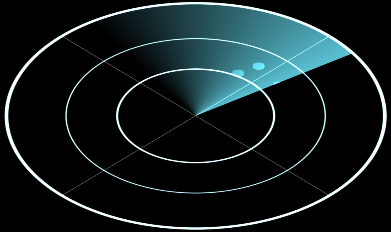
Figure 8.8 – The radar GUI element plots the positions of encounters in terms of their relative distance and angle from the player (at the center of the circle)

Though this section may have been short, it has certainly been full of sweet knowledge and results. There remain several mysteries to uncover regarding the radar mesh texture and its construction, but those will have to await a later chapter of our journey. We come out of this section knowing how to plot polar coordinates as well as how to set up a multi-camera scene with layer masks and Viewports. It’s a nice way to wrap up our work in this area and prepares us for what comes next!

Summary

Let’s take a step back and look at how far we’ve come during this chapter. When we started it, all we had was some route data and a vague idea of what we wanted to happen. Having completed it, we now have a game that can be played from end to end from Route Planning to Driving!

Along the way, we’ve leveraged the Playground to help us define a prototype demo of the driving phase gameplay. It was in that Playground that we learned how to take the raw route data and turn it into a configurable Ribbon mesh with as many or few segments as we’d like. The semi-truck GLB asset was introduced as we learned how to load and prepare assets like this for use in our Scene. Once we learned how to set up the scene, we defined physics and gave our truck the ability to bounce off the route’s walls with MeshImpostor, as well as a way to automatically “kill” the truck if it wanders out of bounds. All that work set us up for smooth integration with the application.

Beginning with a divide-and-conquer approach, we split the code from the Playground up into its different functional areas of responsibility. Then, we hooked up the plumbing to transition from either the splash screen (with the ?testDrive URL Query string) or the onCargoAccepted event of the Route Planning Screen. Having the ability to quickly jump into the driving phase using sample route data made it easy to iterate and test through the rest of the integration with the runtime and input systems.

Our input handling needs for the Driving Phase are different from those of the Planning Phase, so to support that, we added the ability to path the base input action map with an updated set of input-to-action mappings. To keep our space-truck from getting lonely along its route, we turned our attention to hooking up encounters with the Driving screen via routeData.

Once we’d added encounter data to the overall routeData, it was straightforward to use a (for now) sphere mesh as a source for Instances of an Encounter. We’ll be changing this around later, but at this time, we don’t want to arrest any of the hard-earned momenta gained to take on any side-quests. Similarly, we learned how to set up our alternate GUI camera along with the polar coordinates – plotting encounters onto our radar procedural texture/GUI mesh. Put all together, we are in a great place to begin the next chapter in our journey, where we will cover the GUI.

Up until now, we’ve kept our GUI to a minimum. Even so, what amounts to basic boilerplate code while assigning values to properties can be quite astonishing. Nobody wants to have to write all that code and nobody wants to have to maintain it. In the next chapter, we’ll learn how we solve both of those problems while covering some other problems we didn’t even know existed when we go in-depth into the brand-new Babylon.js GUI Editor.

Until then, if you want to spend some more time exploring the ideas and concepts from this chapter, check out the Extended Topics section next for ideas and projects. As always, Space-Truckers: The Discussion Boards at https://github.com/jelster/space-truckers/discussions is the place to ask questions and exchange ideas with fellow Space-Truckers, while the Babylon.js forums are where to engage with the greater Babylon.js community. See a problem with the code or have an idea you’d like to see implemented? Feel free to create an Issue in the Space-Truckers repository!

Extended Topics

The following are some extended topics for you to try out:

• Add an “encounter warning” UI indication whenever the truck is within a set distance of an encounter
• When the ship hits the side of the wall, play an appropriate sound effect. The volume of the played effect should scale with the energy of the impact. Bonus points for spatially locating the sound at the location of the collision.
• An Encounter Table implies something static. Make encounters more dynamic by loading the list of potential encounters from a remote index repository hosted on GitHub. Community members can contribute new encounters by submitting a Pull Request containing the new encounter’s definition. Once accepted and merged, the encounter becomes available to be used in a game session.
• As a prerequisite for the preceding bullet, adding the ability for each encounter to use a different mesh/material combination is a necessity. Read the mesh URL from the encounter data but be careful that you’re not creating new meshes/materials for every instance of an encounter!
• Another Encounter feature could be the ability for each encounter type to define and control its behavior. An easy and cool way to do this is outlined in the very next chapter in the Advanced Coroutine Usage section.