
Chapter 5: Data Transformation and Processing with Synapse Notebooks
In this chapter, we will cover how to do data processing and transformation with Synapse notebooks. Details on using pandas DataFrames within Synapse notebooks will be covered, which will help us to explore data that is stored as Parquet files in Azure Data Lake Storage (ADLS) Gen2 as a pandas DataFrame and then write it back to ADLS Gen2 as a Parquet file.
We will be covering the following recipes:
- Landing data in ADLS Gen2
- Exploring data with ADLS Gen2 to pandas DataFrame in Synapse notebook
- Processing data from a PySpark notebook within Synapse
- Performing read-write operations to a Parquet file using Spark in Synapse
- Analytics with Spark
Landing data in ADLS Gen2
In this recipe, we will learn how to create an ADLS Gen2 storage account and upload data as a Parquet file, where ADLS Gen2 can be considered as the landing zone before data is processed and transformed.
Getting ready
We will be using a public dataset for our scenario. This dataset will consist of New York yellow taxi trip data; this includes attributes such as trip distances, itemized fares, rate types, payment types, pick-up and drop-off dates and times, driver-reported passenger counts, and pick-up and drop-off locations. We will be using this dataset throughout this recipe to demonstrate various use cases:
- To get the dataset, you can go to the following URL: https://www.kaggle.com/microize/newyork-yellow-taxi-trip-data-2020-2019.
- The code for this recipe can be downloaded from the GitHub repository: https://github.com/PacktPublishing/Analytics-in-Azure-Synapse-Simplified.
Let's get started.
How to do it…
ADLS Gen2 is a data lake solution providing capabilities to store filesystems in a hierarchical namespace and low-cost object-based storage with guaranteed high availability and disaster recovery features. The Azure Blob Filesystem (ABFS) driver provides the necessary interface for ADLS Gen2 storage. Our input dataset will be stored as a Parquet file in ADLS Gen2 inside a container and subsequently used for data standardization, processing, and transformation with Synapse notebooks.
Let's create an ADLS Gen2 storage account to start:
- Log in to the Azure portal: https://portal.azure.com/#home.
- Navigate to Storage accounts by using the top search bar, where you can search for resources, services, and docs.
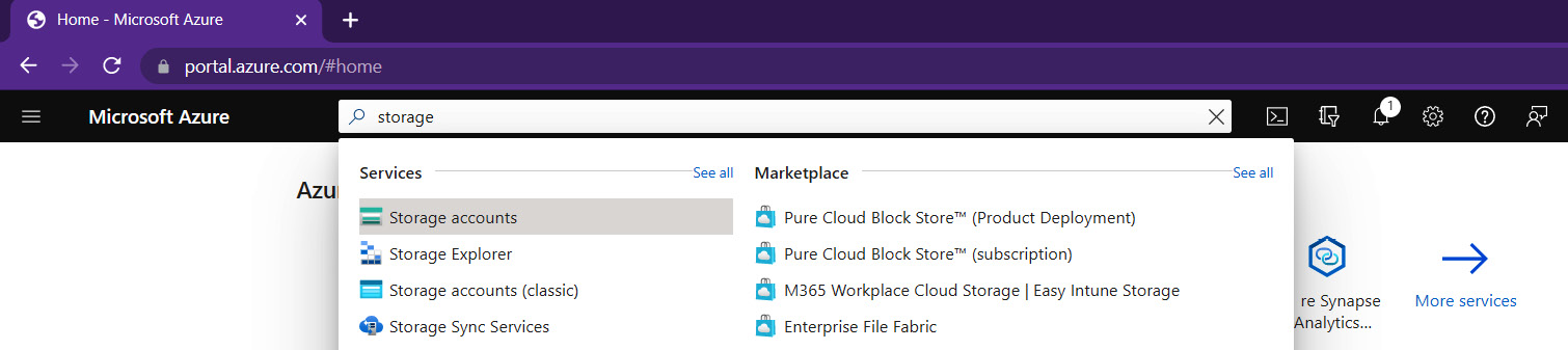
Figure 5.1 – Searching for Storage accounts
- Click on Create storage account.
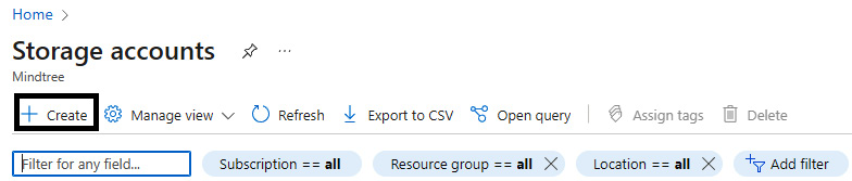
Figure 5.2 – Create storage account
- On the Basics tab, choose the subscription and for the resource group details select SynapseRG, as shown in the following screenshot:
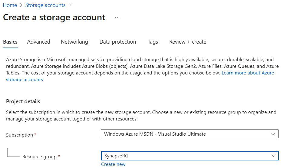
Figure 5.3 – Create a storage account – Basics tab
- Enter the storage account name as synapsecookbookdemo. Choose the region, but leave Performance as Standard.
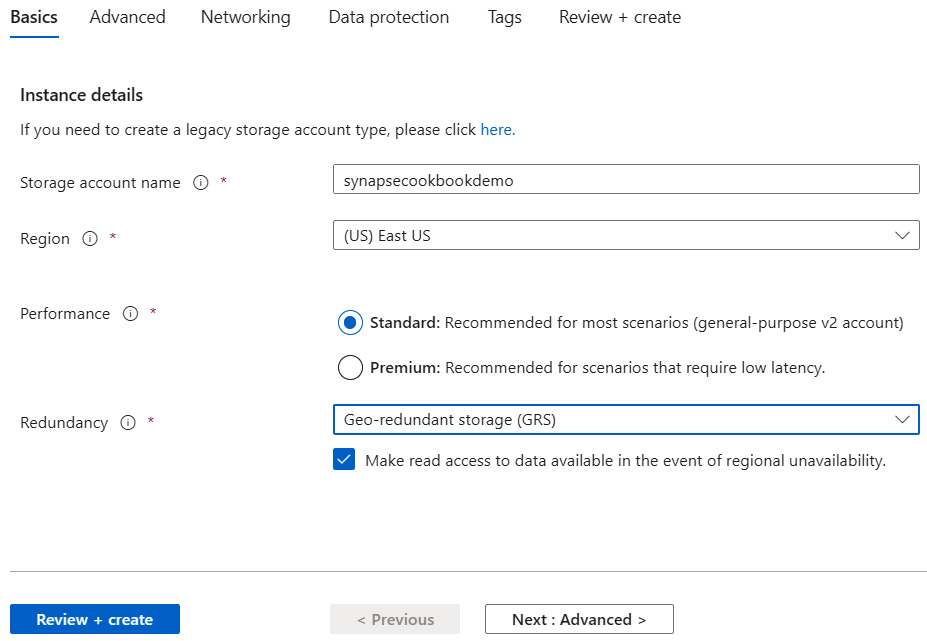
Figure 5.4 – Create a storage account – Basics tab
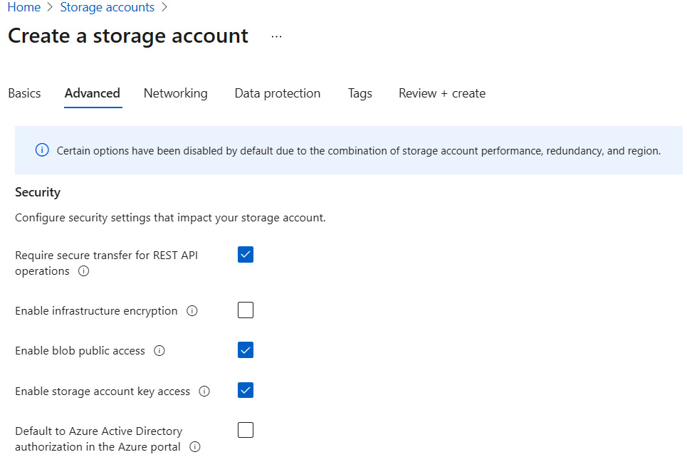
Figure 5.5 – Create a storage account – Advanced tab
- Check Enable hierarchical namespace, which will accelerate the big data analytics workload and help us to enable file-level access control lists.
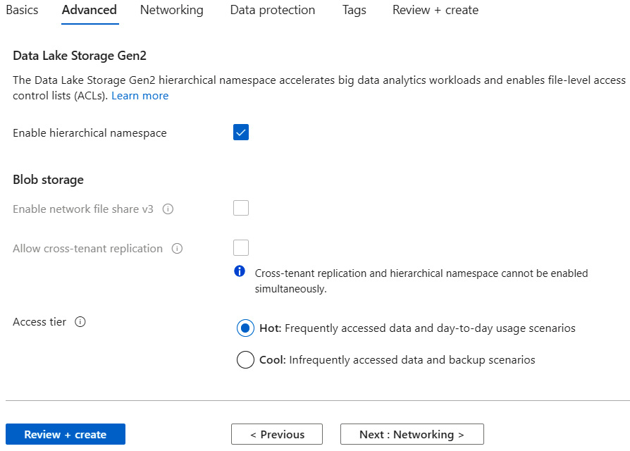
Figure 5.6 – Create a storage account – Advanced tab
- Create the tags and review the page, then create the storage account.
- Go to the Access Control (IAM) page, click Add role assignment (Preview), and on the Add role assignment page, assign a role to the users.
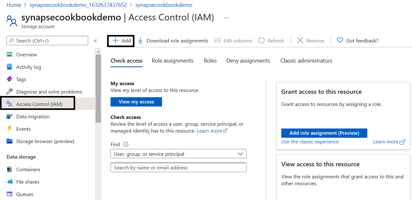
Figure 5.7 – Create a storage account – Access Control (IAM)
- In the Role field, select Reader or Contributor.
- To add or remove role assignments, we need to have write and delete permissions, such as an Owner role.
- In the Assign access to field, select User, group, or service principal.
- In the Select field, select the user that requires access to the storage account.
- Click Save.
If you want to add multiple users to access the storage account, you must perform the same steps for each user.
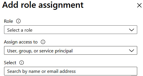
Figure 5.8 – Create a storage account – IAM role assignment
We have created a storage account in ADLS Gen2, enabled a hierarchical namespace for storage, and enabled role assignment, so we can now proceed to the next step.
Let's create a container in ADLS Gen2 now.
- Add a container to the storage account that we created in step 8.
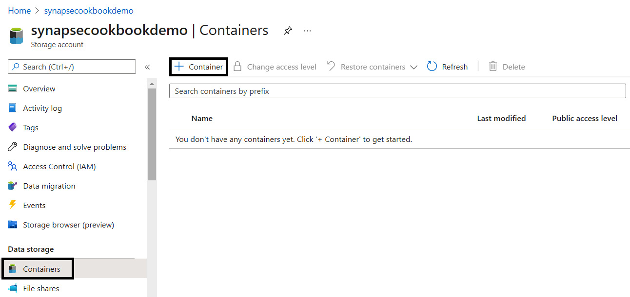
Figure 5.9 – Create a storage account – list of containers
- Provide a name for the container and create it.
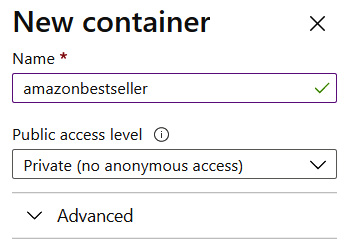
Figure 5.10 – Create a storage account – New container
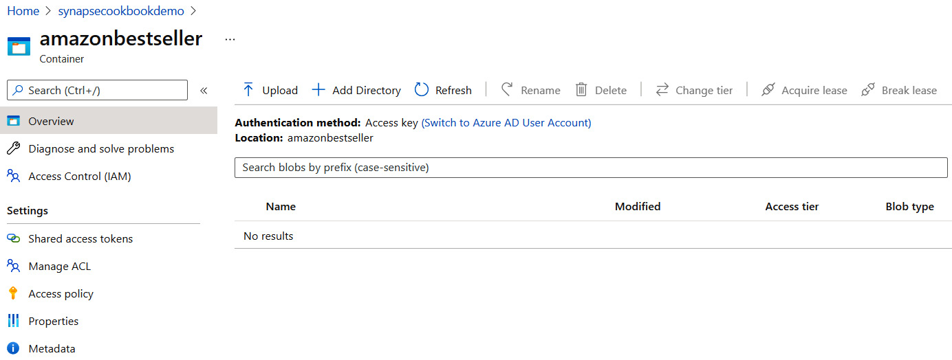
Figure 5.11 – Create a storage account – containers page
- Upload the Parquet file to the container.
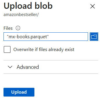
Figure 5.12 – Create a storage account – Upload blob
The data is now in our ADLS Gen2 data lake, inside a container as a Parquet file.
Exploring data with ADLS Gen2 to pandas DataFrame in Synapse notebook
In this recipe, we will learn how to create a Synapse Analytics workspace and create Synapse notebooks so that we can load data from an ADLS Gen2 Parquet file to a pandas DataFrame. Synapse notebooks are required for us to perform a detailed analysis of data in interactive session mode.
Getting ready
We will be using a public dataset for our scenario. This dataset will consist of New York yellow taxi trip data; this includes attributes such as trip distances, itemized fares, rate types, payment types, pick-up and drop-off dates and times, driver-reported passenger counts, and pick-up and drop-off locations. We will be using this dataset throughout this recipe to demonstrate various use cases:
- To get the dataset, you can go to the following URL: https://www.kaggle.com/microize/newyork-yellow-taxi-trip-data-2020-2019.
- The code for this recipe can be downloaded from the GitHub repository: https://github.com/PacktPublishing/Analytics-in-Azure-Synapse-Simplified.
Let's get started.
How to do it…
Exploring an ADLS Gen2 Parquet file in a pandas DataFrame requires us to create a Synapse Analytics workspace, a Synapse Spark pool, and a Synapse notebook. The following recipe is a step-by-step guide to using the core features of Synapse Analytics.
Creating a Synapse Analytics workspace
Synapse Analytics workspace creation requires us to create a resource group or have access to an existing resource group with owner permissions. Let's use an existing resource group, where you will find owner permissions for the user:
- Log in to the Azure portal: https://portal.azure.com/#home.
- Search for Azure Synapse Analytics by using the top search bar, where you can search for resources, services, and docs.
- Select Azure Synapse Analytics.
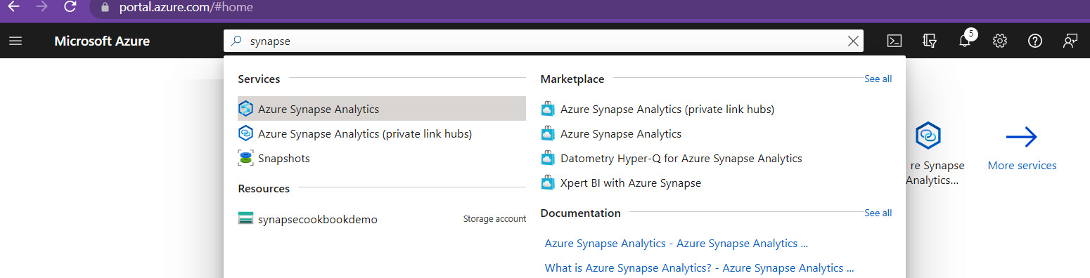
Figure 5.13 – Searching for Azure Synapse Analytics
- Create an Azure Synapse Analytics workspace using either the Create button or the Create Synapse workspace button.
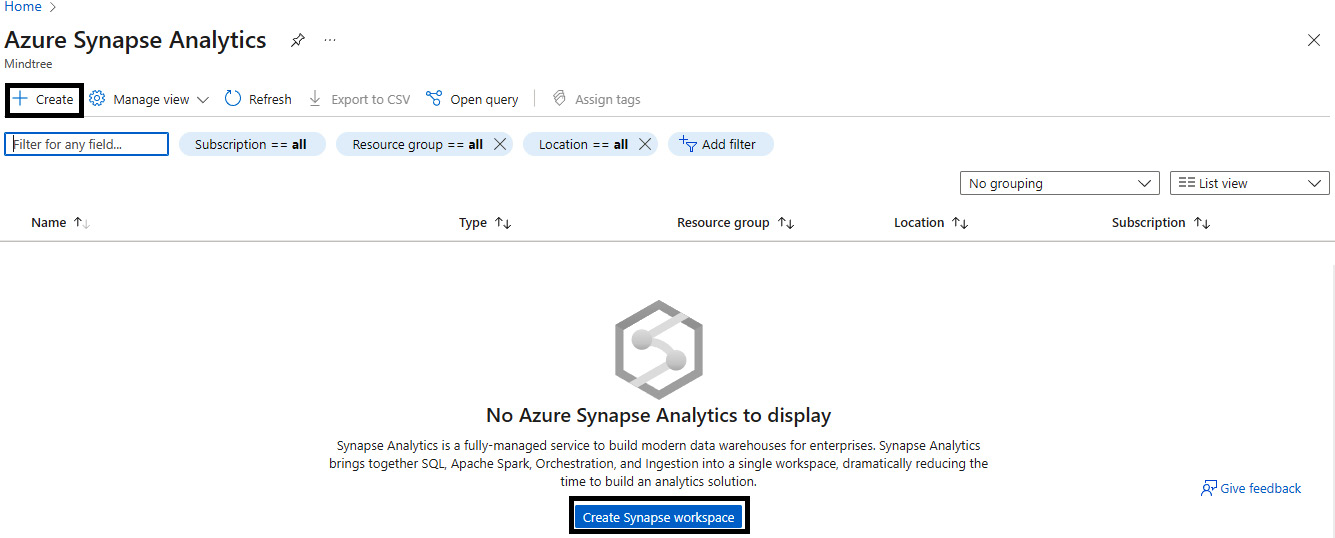
Figure 5.14 – Create Synapse workspace
- On the Basics tab, enter the resource group and the workspace name as synapsecookbook.
- Associate it with the ADLS Gen2 account name and the container that we created in the previous recipe.
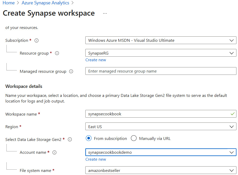
Figure 5.15 – Create Synapse workspace – Basics tab
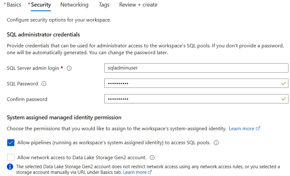
Figure 5.16 – Create Synapse workspace – Security tab
Creating a Synapse Spark pool
Synapse Spark pools are the home for all Spark resources, notebooks, and clusters. When we create a Spark pool, a Spark session is created by default. This Spark pool takes care of Spark resources that will be used by the Spark session. The user can work with the Spark pool without the need to manage clusters because the Synapse workspace takes care of this, removing the overhead for users to manage it by themselves:
- Open the Synapse workspace that we created earlier and select Apache Spark pools. Click New to create a new Synapse Spark pool.
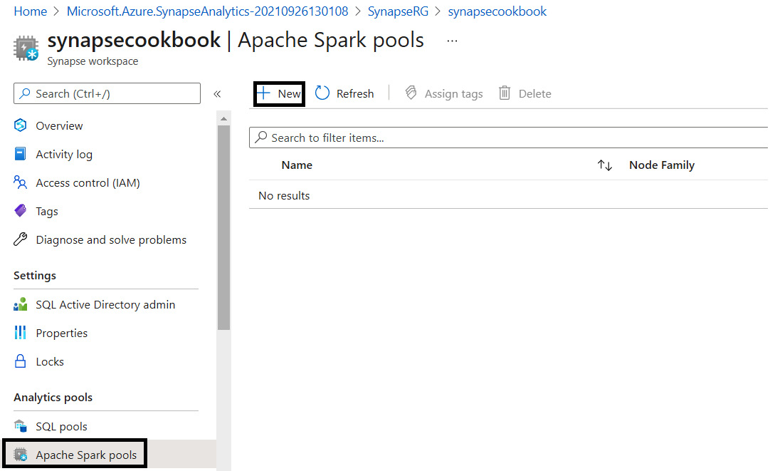
Figure 5.17 – Creating a Synapse Spark pool
- On the Basics tab, enter a Spark pool name and select the desired node size. Review and create the whole setup.
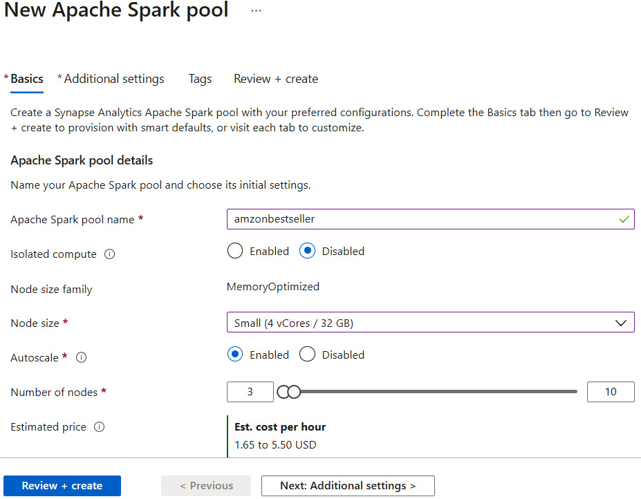
Figure 5.18 – Creating a Synapse Spark pool – Basics tab
The Spark pool is successfully created now, so we can proceed with notebook creation and execution.
Creating a Synapse notebook
Synapse notebooks are interactive Spark sessions and editors for the user to work on Spark code:
- Go to Synapse Studio and create a new notebook, as shown in the following screenshot:
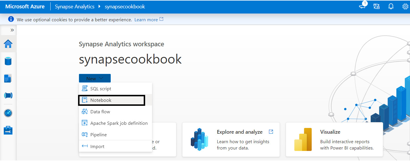
Figure 5.19 – Synapse Analytics Studio
- Attach the notebook to the Spark pool that we created earlier and run the cell. It starts an Apache Spark session; we are now ready to code in PySpark.
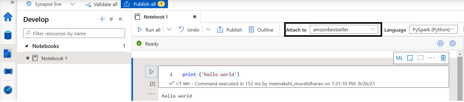
Figure 5.20 – Creating a Synapse notebook
- Copy the ABFS path of the Parquet file from the storage account. In the code cell, copy and paste the following Python code to read the Parquet file as a DataFrame and convert it to pandas:
df = spark.read.parquet('abfss://[email protected]/NYCTripSmall.parquet')
df.show(10)
print('Converting to Pandas.')
pd = df.toPandas()
print(pd)
You can view the following output in pandas on a Synapse notebook screen:
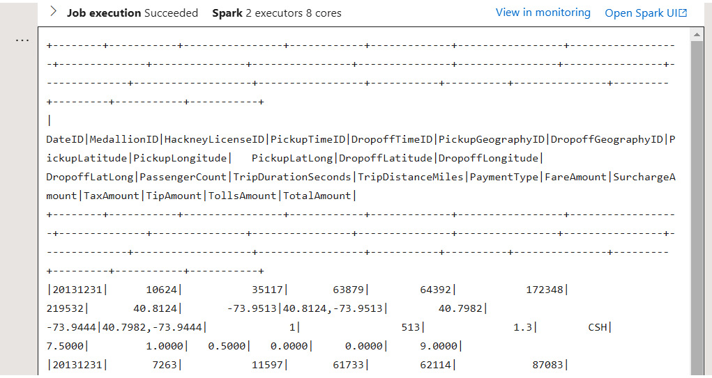
Figure 5.21 – pandas output
There's more…
Alternatively, we can directly read Parquet files into pandas, as follows:
Import pandas
df = pandas.read_parquet('abfss://[email protected]/NYCTripSmall.parquet')
print(df)
Processing data from a PySpark notebook within Synapse
In this section, we will learn how to process and view data as charts with different operations of DataFrame using PySpark in Synapse notebooks. Charts are usually used to display data and help us to understand patterns between different data points. Graphs and diagrams also help to compare data.
Getting ready
We will be using a public dataset for our scenario. This dataset will consist of New York yellow taxi trip data; this includes attributes such as trip distances, itemized fares, rate types, payment types, pick-up and drop-off dates and times, driver-reported passenger counts, and pick-up and drop-off locations. We will be using this dataset throughout this recipe to demonstrate various use cases:
- To get the dataset, you can go to the following URL: https://www.kaggle.com/microize/newyork-yellow-taxi-trip-data-2020-2019.
- The code for this recipe can be downloaded from the GitHub repository: https://github.com/PacktPublishing/Analytics-in-Azure-Synapse-Simplified.
How to do it…
Let's get started:
- View the schema of the input dataset. Read the Parquet file as a DataFrame and view the schema using the printSchema method of the DataFrame:
df = spark.read.parquet('abfss://[email protected]/NYCTripSmall.parquet')
df.printSchema()
The output is shown in the following screenshot:
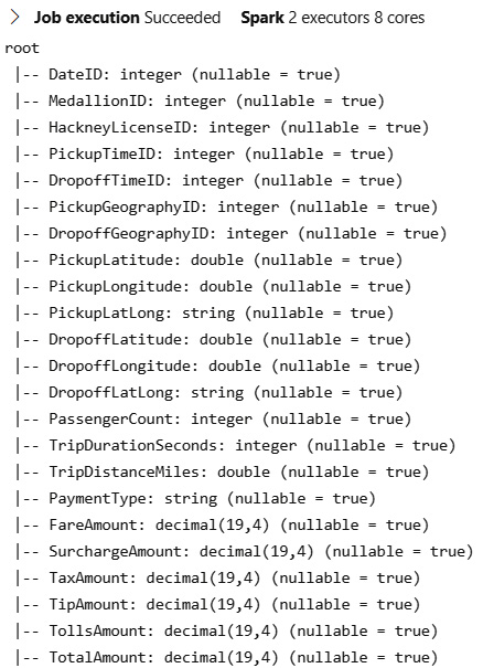
Figure 5.22 – Reading from a Parquet file
- View the records in a DataFrame. The DataFrame's show method, applied to a number of records, helps us to view the records in the DataFrame. Disable truncation with the truncate statement to view all the records fully:
df.show(5, truncate=false)
Figure 5.23 shows the output:
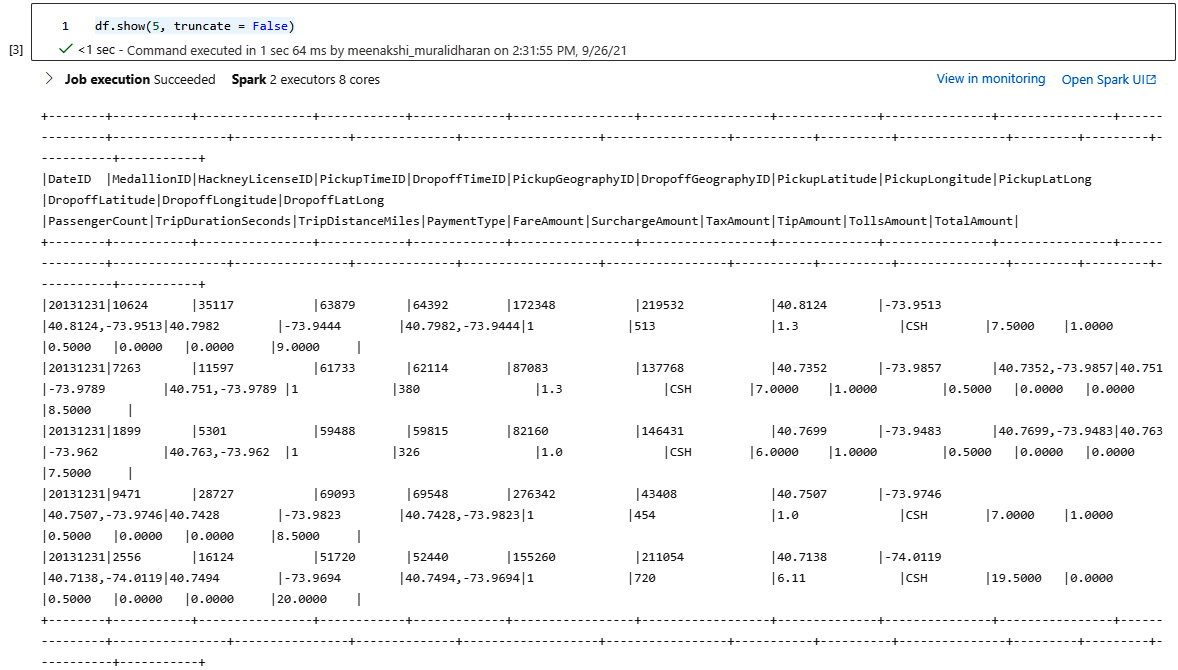
Figure 5.23 – Output of the DataFrame
- View selected columns of the DataFrame. Select the desired columns using the select method and view the results with the show method:
df.select('PassengerCount', 'DateID').show(10)
The output is shown in the following screenshot:
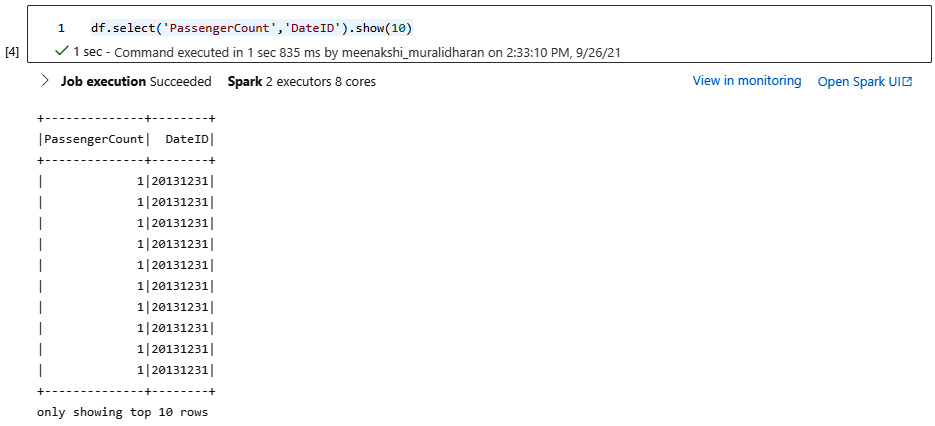
Figure 5.24 – Passenger output
- Use the groupBy clause and sort the records in a DataFrame. Group by any of the desired columns and sort the results in ascending order:
df.groupBy("DateID").count().sort("count", ascending=True).show()
The following screenshot shows the output:
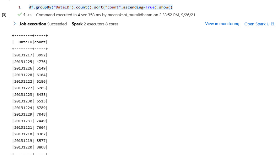
Figure 5.25 – Datewise count of trips
- View descriptive statistical results of the DataFrame. Descriptive or summary statistics of a DataFrame can be viewed using the count, min, max, mean, and stddev functions supported by PySpark. describe will perform all summary statistics and show the results of the DataFrame:
df.describe().show()
The following screenshot shows the results:
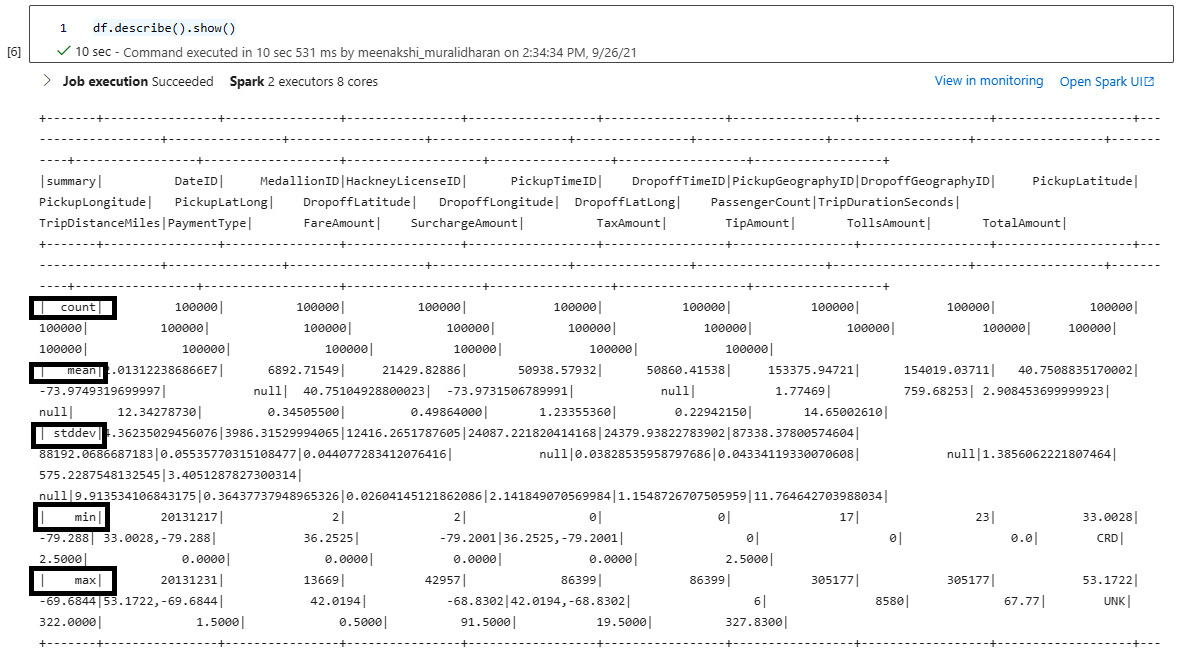
Figure 5.26 – Statistical results of the DataFrame
- Filter a column in the DataFrame. Filter the results of a column using the filter function. The following code filters the DataFrame where TripDistanceMiles is greater than 1.5 miles and displays all the records:
df.filter(df.TripDistanceMiles > 1.5).count()
Figure 5.27 displays the result:
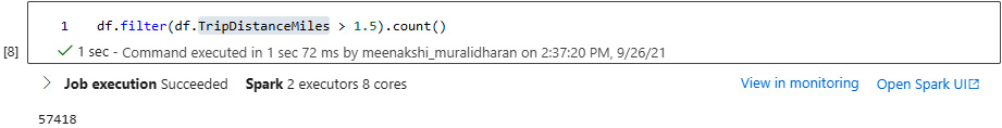
Figure 5.27 – Filter trip distance greater than 1.5 miles
- Add a column to the DataFrame. A new column can be added to the DataFrame using withColumn. The following code shows a column named Longtrip being added to the DataFrame:
from pyspark.sql.functions import *
df=df.withColumn("Longtrip", col("TripDistanceMiles"))
df.show(5)
The output is shown in the following screenshot:
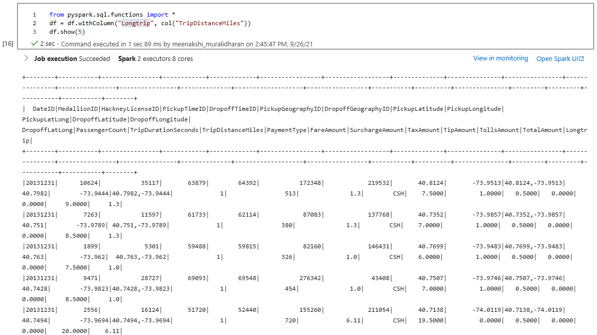
Figure 5.28 – Adding a new column to the DataFrame
- Filter trip data to trips between 1 and 3 miles. We can filter the trip data to where the travel distance is within 1 to 3 miles and display the records:
df.filter(df["Longtrip"].between(1,3)).show(5)
The following screenshot shows the results:
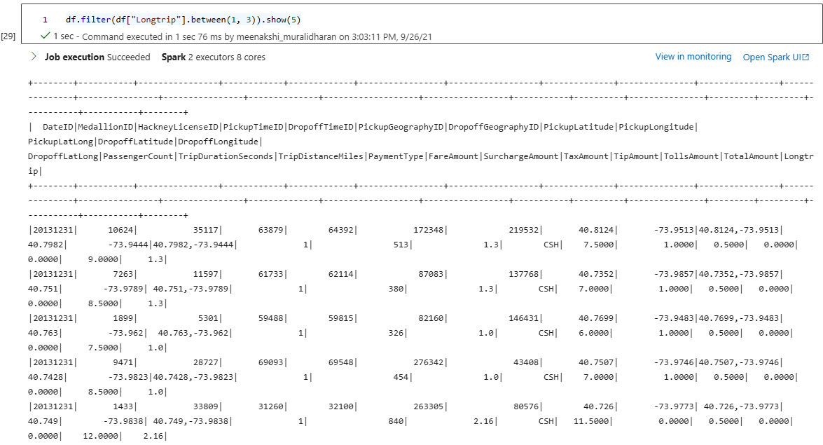
Figure 5.29 – Filtering to trips between 1 and 3 miles
- View in a chart. We can select the Chart option in the Synapse notebook and view the data in a bar chart:
df=df.groupby("DateID").agg({'TotalAmount':"sum"})
display(df)
The following screenshot shows the output:

Figure 5.30 – Viewing a bar chart
Select the chart settings with the following code and change to a pie chart to get a clear picture of the data:
df=df.groupby("DateID").agg({'TotalAmount':"sum"})
display(df)
The result is shown in the following screenshot:
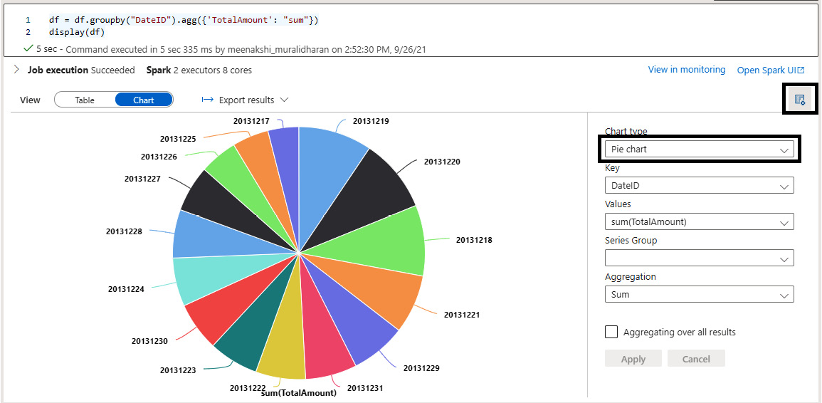
Figure 5.31 – Viewing the pie chart
Performing read-write operations to a Parquet file using Spark in Synapse
Apache Parquet is a columnar file format that is supported by many big data processing systems and is the most efficient file format for storing data. Most of the Hadoop and big data world uses Parquet to a large extent. The advantage is the efficient data compression support, which enhances the performance of complex data.
Spark supports both reading and writing Parquet files because it reduces the underlying data storage. Since it occupies less storage, it actually reduces I/O operations and consumes less memory.
In this section, we will learn about reading Parquet files and writing to Parquet files. Reading and writing to a Parquet file with PySpark code is straightforward.
Getting ready
We will be using a public dataset for our scenario. This dataset will consist of New York yellow taxi trip data; this includes attributes such as trip distances, itemized fares, rate types, payment types, pick-up and drop-off dates and times, driver-reported passenger counts, and pick-up and drop-off locations. We will be using this dataset throughout this recipe to demonstrate various use cases:
- To get the dataset, you can go to the following URL: https://www.kaggle.com/microize/newyork-yellow-taxi-trip-data-2020-2019.
- The code for this recipe can be downloaded from the GitHub repository: https://github.com/PacktPublishing/Analytics-in-Azure-Synapse-Simplified.
How to do it…
Let's get started:
- Use spark.read.parquet to read Parquet files from ABFS storage in ADLS Gen2. The files are read as a DataFrame. Use the DataFrame's write.parquet method to write Parquet files and specify the ABFS storage path.
The following code snippet performs the operation of reading and writing to Parquet files:
df = spark.read.parquet('abfss://[email protected]/NYCTripSmall.parquet')
from pyspark.sql.functions import *
df = df.withColumn("Longtrip", col("TripDistanceMiles"))
df.write.parquet('abfss://[email protected]/NYCTripSmallwrite.parquet')
dfwrite = spark.read.parquet('abfss://[email protected]/NYCTripSmallwrite.parquet')
dfwrite.show(5)
- Go to Synapse Studio, choose storage, and navigate to the Linked tab server, where the storage account can be accessed.
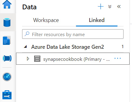
Figure 5.32 – Storage account from Synapse Studio
- The New York taxi Parquet file has write in the filename for identification in our code, as you can see in the following screenshot, stored in the ADLS Gen2 filesystem:
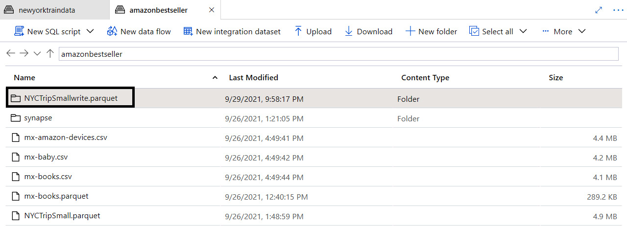
Figure 5.33 – Viewing the Parquet file written in code in the storage account
Analytics with Spark
In this section, we will learn how to do exploratory analysis with a dataset using PySpark in Synapse notebooks.
Getting ready
We will be using a public dataset for our scenario. This dataset will consist of New York yellow taxi trip data; this includes attributes such as trip distances, itemized fares, rate types, payment types, pick-up and drop-off dates and times, driver-reported passenger counts, and pick-up and drop-off locations. We will be using this dataset throughout this recipe to demonstrate various use cases:
- To get the dataset, you can go to the following URL: https://www.kaggle.com/microize/newyork-yellow-taxi-trip-data-2020-2019.
- The code for this recipe can be downloaded from the GitHub repository: https://github.com/PacktPublishing/Analytics-in-Azure-Synapse-Simplified.
How it works…
Let's get started and try to find out the busiest day of the week with the most trips:
- Read the Parquet file in the Synapse notebook. The trip data is read from ADLS Gen2 into a DataFrame using spark.read.parquet:
dftrip = spark.read.parquet('abfss://[email protected]/NYCTripSmall.parquet')
- Add a new date column to analyze the data. A trip_date date column is added and the existing DateID column, which is a string, is converted to date format, yyyyMMdd. The schema is analyzed to check whether the new column is added:
from pyspark.sql import functions as F
dftrip=dftrip.withColumn("trip_date", F.to_date(F.col("DateID").cast("string"),'yyyyMMdd'))
dftrip.printSchema()
The following screenshot shows the results:
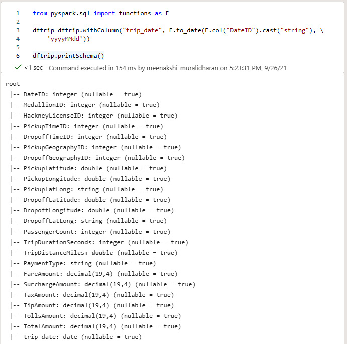
Figure 5.34 – Adding a date column
- Analyze the day, month, and year of the date column. Date functions are effectively used to analyze the day of the week, day of the month, and day of the year so that the whole DataFrame provides more information:
dftrip.select(col("trip_date"),
dayofweek(col("trip_date")).alias("dayofweek"),
dayofmonth(col("trip_date")).alias("dayofmonth"),
dayofyear(col("trip_date")).alias("dayofyear"),
).show()
The output is shown in the following screenshot:
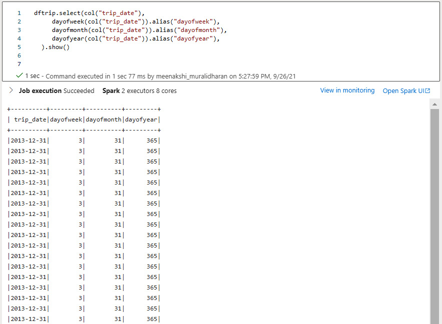
Figure 5.35 – Viewing the day of the week, month, and year
- Add a day column and find out the day of the trip. A day column is added and the trip_date column is used to derive the day of the week. The date_format function helps to display the day of the week, which will be used for our calculation:
import pyspark.sql.functions as f
dftrip=dftrip.withColumn('Day', f.date_format('trip_date', 'E'))
dftrip.show(5)
The following screenshot shows the result:
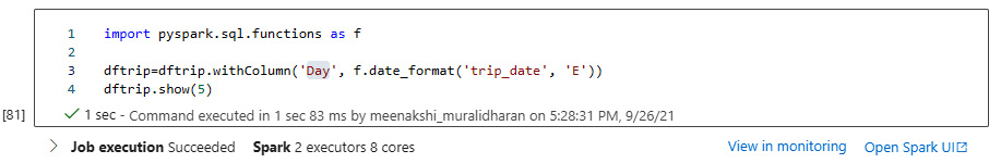
Figure 5.36 – Adding a new Day column
- Analyze the most trips in a day of the week. The DataFrame is grouped by the Day column and the overall count is displayed to find out the most trips in a day of the week. Tuesdays are the day of the week when the most trips take place:
dftrip.groupBy("Day").count().orderBy("count").show(7)
The following screenshot shows the output:
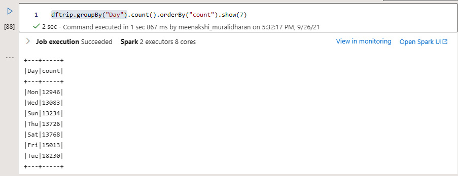
Figure 5.37 – Finding the most trips in a week
- Display a chart showing trips on a day of the week. The chart displayed clearly indicates that Tuesdays are the busiest day of the week:
dftrip=dftrip.agg({'Day':"count"})
display(dftrip)
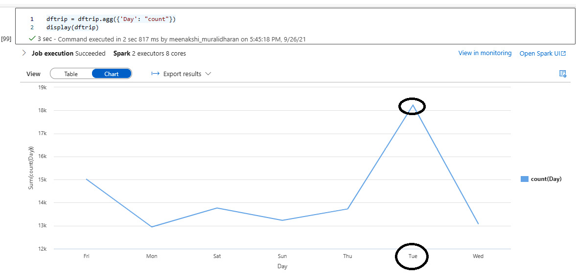
Figure 5.38 – View in a line chart