11
The Toolz Package
The toolz package, offered by the pytoolz project on GitHub, contains a number of functional programming features. Specifically, these libraries offer iteration tools, higher-order function tools, and even some components to work with stateful dictionaries in an otherwise stateless function application.
There is some overlap between the toolz package and components of the standard library. The toolz project decomposes into three significant parts: itertoolz, functoolz, and dicttoolz. The itertoolz and functoolz modules are designed to mirror the standard library modules itertools and functools.
We’ll look at the following list of topics in this chapter:
We’ll start with star-mapping, where a
f(*args)is used to provide multiple arguments to a mappingWe’ll also look at some additional
functools.reduce()topics using theoperatormoduleWe’ll look at the
toolzpackage, which provides capabilities similar to the built-initertoolsandfunctoolspackages, but offers a higher level of functional purityWe’ll also look at the
operatormodule and how it leads to some simplification and potential clarification when defining higher-order functions
We’ll start with some more advanced use of itertools and functools.reduce(). These two topics will introduce the use cases for the toolz package.
11.1 The itertools star map function
The itertools.starmap() function is a variation of the map() higher-order function. The map() function applies a function against each item from a sequence. The starmap(f, S) function presumes each item, i, from the sequence, S, is a tuple, and uses f(*i). The number of items in each tuple must match the number of parameters in the given function.
Here’s an example that uses a number of features of the starmap() function:
>>> from itertools import starmap, zip_longest
>>> d = starmap(pow, zip_longest([], range(4), fillvalue=60))
>>> list(d)
[1, 60, 3600, 216000]
The itertools.zip_longest() function will create a sequence of pairs, [(60, 0), (60, 1), (60, 2), (60, 3)]. It does this because we provided two sequences: the [] brackets and the range(4) parameter. The fillvalue parameter is used when the shorter sequence runs out of data.
When we use the starmap() function, each pair becomes the argument to the given function. In this case, we used the the built-in pow() function, which is the ** operator (we can also import this from the operator() module; the definition is in both places). This expression calculates values for [60**0, 60**1, 60**2, 60**3]. The value of the d variable is [1, 60, 3600, 216000].
The starmap() function expects a sequence of tuples. We have a tidy equivalence between the map(f, x, y) and starmap(f, zip(x, y)) functions.
Here’s a continuation of the preceding example of the itertools.starmap() function:
>>> p = (3, 8, 29, 44)
>>> pi = sum(starmap(truediv, zip(p, d)))
>>> pi
3.1415925925925925
We’ve zipped together two sequences of four values. The value of the d variable was computed above using starmap(). The p variable refers to a simple list of literal items. We zipped these to make pairs of items. We used the starmap() function with the operator.truediv() function, which is the / operator. This will compute a sequence of fractions that we sum. The sum is an approximation of π ≈![]() +
+ ![]() +
+ ![]() +
+ ![]() .
.
Here’s a slightly simpler version that uses the map(f, x, y) function instead of the starmap(f, zip(x,y)) function:
>>> pi = sum(map(truediv, p, d))
>>> pi
3.1415925925925925
In this example, we effectively converted a base 60 fractional value to base 10. The sequence of values in the d variable are the appropriate denominators. A technique similar to the one explained earlier in this section can be used to convert other bases.
Some approximations involve potentially infinite sums (or products). These can be evaluated using similar techniques explained previously in this section. We can leverage the count() function in the itertools module to generate an arbitrary number of terms in an approximation. We can then use the takewhile() function to only accumulate values that contribute a useful level of precision to the answer. Looked at another way, takewhile() yields a stream of significant values, and stops consuming values from the stream when an insignificant value is found.
For our next example, we’ll leverage the fact() function defined in Chapter 6, Recursions and Reductions. Look at the Implementing manual tail-call optimization section for the relevant code.
We’ll introduce a very similar function, the semifactorial, also called double factorial, denoted by the !! symbol. The definition of semifactorial is similar to the definition of factorial. The important difference is that it is the product of alternate numbers instead of all numbers. For example, take a look at the following formulas:
5!! = 5 × 3 × 1
7!! = 7 × 5 × 3 × 1
Here’s the essential function definition:
def semifact(n: int) -> int:
    match n:
        case 0 | 1:
            return 1
        case 2:
            return 2
        case _:
            return semifact(n-2)*n
Here’s an example of computing a sum from a potentially infinite sequence of fractions using the fact() and semifact() functions:
>>> from Chapter06.ch06_ex1 import fact
>>> from itertools import count, takewhile
>>> num = map(fact, count())
>>> den = map(semifact, (2*n+1 for n in count()))
>>> terms = takewhile(
... lambda t: t > 1E-10, map(truediv, num, den))
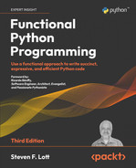
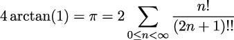
>>> round(float(2*sum(terms)), 8)
3.14159265The num variable is a potentially infinite sequence of numerators, based on the fact() function. The count() function returns ascending values, starting from zero and continuing indefinitely. The den variable is also a potentially infinite sequence of denominators, based on the semifactorial function. This den computation also uses count() to create a potentially infinite series of values.
To create terms, we used the map() function to apply the operator.truediv() function, the / operator, to each pair of values. We wrapped this in a takewhile() function so that we only take terms from the map() output while the value is greater than some relatively small value, in this case, 10−10.
This is a series expansion based on this definition:
An interesting variation of the series expansion theme is to replace the operator.truediv() function with the fractions.Fraction() function. This will create exact rational values that don’t suffer from the limitations of floating-point approximations. We’ve left the implementation as an exercise for the reader.
All the built-in Python operators are available in the operator module. This includes all of the bit-fiddling operators as well as the comparison operators. In some cases, a generator expression may be more succinct or expressive than a rather complicated-looking starmap() function with a function that represents an operator.
The operator module offers functions that can be more terse than a lambda. We can use the operator.add method instead of the add=lambda a, b: a+b form. If we have expressions more complex than a single operator, then the lambda object is the only way to write them.
11.2 Reducing with operator module functions
We’ll look at one more way that we can use the operator module definitions: we can use them with the built-in functools.reduce() function. The sum() function, for example, can be implemented as follows:
sum = functools.partial(functools.reduce, operator.add)This creates a partially evaluated version of the reduce() function with the first argument supplied. In this case, it’s the + operator, implemented via the operator.add() function.
If we have a requirement for a similar function that computes a product, we can define it like this:
prod = functools.partial(functools.reduce, operator.mul)This follows the pattern shown in the previous example. We have a partially evaluated reduce() function with the first argument of the * operator, as implemented by the operator.mul() function.
It’s not clear whether we can do similar things with too many of the other operators. We might be able to find a use for the operator.concat() function.
The and() and or() functions are the bit-wise & and | operators. These are designed to create integer results.
If we want to perform a reduce using the proper Boolean operations, we should use the all() and any() functions instead of trying to create something with the reduce() function.
Once we have a prod() function, this means that the factorial can be defined as follows:
fact = lambda n: 1 if n < 2 else n * prod(range(1, n))This has the advantage of being succinct: it provides a single-line definition of factorial. It also has the advantage of not relying on recursion and avoids any problem with stack limitations.
It’s not clear that this has any dramatic advantages over the many alternatives we have in Python. However, the concept of building a complex function from primitive pieces such as the partial() and reduce() functions and the operator module is very elegant. This is an important design strategy for writing functional programs.
Some of the designs can be simplified by using features of the toolz package. We’ll look at some of the toolz package in the next section.
11.3 Using the toolz package
The toolz package comprises functions that are similar to some of the functions in the built-in itertools and functools modules. The toolz package adds some functions to perform sophisticated processing on dictionary objects. This package has a narrow focus on iterables, dictionaries, and functions. This overlaps nicely with the data structures available in JSON and CSV documents. The idea of processing iterables that come from files or databases allows a Python program to deal with vast amounts of data without the complication of filling memory with the entire collection of objects.
We’ll look at a few example functions from the various subsections of the toolz package. There are over sixty individual functions in the current release. Additionally, there is a cytoolz implementation written in Cython that provides higher performance than the pure Python toolz package.
11.3.1 Some itertoolz functions
We’ll look at a common data analysis problem of cleaning and organizing data from a number of datasets. In Chapter 9, Itertools for Combinatorics – Permutations and Combinations, we mentioned several datasets available at https://www.tylervigen.com.
Each correlation includes a table of the relevant data. The tables often look like the following example:
| 2000 | 2001 | 2002 | ... | |
| Per capita consumption of cheese (US) | 29.8 | 30.1 | 30.5 | ... |
| Number of people who died by becoming | ||||
| tangled in their bedsheets | 327 | 456 | 509 | ... |
There are generally three rows of data in each example of a spurious correlation. Each row has 10 columns of data, a title, and an empty column that acts as a handy delimiter. A small parsing function, using Beautiful Soup, can extract the essential data from the HTML. This extract isn’t immediately useful; more transformations are required.
Here’s the core function for extracting the relevant text from HTML:
from bs4 import BeautifulSoup  # type: ignore[import]
import urllib.request
from collections.abc import Iterator

def html_data_iter(url: str) -> Iterator[str]:
    with urllib.request.urlopen(url) as page:
        soup = BeautifulSoup(page.read(), ’html.parser’)
        data = soup.html.body.table.table
        for subtable in data.table:
            for c in subtable.children:
                yield c.text
This html_data_iter() function uses urllib to read the HTML pages. It creates a BeautifulSoup instance from the raw data. The soup.html.body.table.table expression provides a navigation path into the HTML structure. This digs down into nested <table> tags to locate the data of interest. Within the nested table, there will be other sub-tables that contain rows and columns. Because the various structures can be somewhat inconsistent, it seems best to extract the text and impose a meaningful structure on the text separately.
This html_data_iter() function is used like this to acquire data from an HTML page:
>>> s7 = html_data_iter("http://www.tylervigen.com/view_correlation?id=7")The result of this expression is a sequence of strings of text. Many examples have 37 individual strings. These strings can can be divided into 3 rows of 12 strings and a fourth row with a single string value. We can understand these rows as follows:
The first row has an empty string, ten values of years, plus one more zero-length string.
The second row has the first data series title, ten values, and an extra zero-length string.
The third row, like the second, has the second data series title, ten values, and an extra string.
A fourth row has a single string with the correlation value between the two series.
This requires some reorganization to create a set of sample values we can work with.
We can use toolz.itertoolz.partition to divide the sequence of values into groups of 12. If we interleave the three collections using toolz.itertoolz.interleave, it will create a sequence with a value from each of the three rows: year, series one, and series two. If this is partitioned into groups of three, each year and the two sample values will be a small three-tuple. We’ll quietly drop the additional row with the correlation value.
This isn’t the ideal form of the data, but it gets us started on creating useful objects. In the long run, the toolz framework encourages us to create dictionaries to contain the sample data. We’ll get to the dictionaries later. For now, we’ll start with rearranging the source data of the first 36 strings into 3 groups of 12 strings, and then 12 groups of 3 strings. This initial restructuring looks like this:
>>> from toolz.itertoolz import partition, interleave

>>> data_iter = partition(3, interleave(partition(12, s7)))
>>> data = list(data_iter)

>>> from pprint import pprint
>>> pprint(data)
[(’’,
  ’Per capita consumption of cheese (US)Pounds (USDA)’,
  ’Number of people who died by becoming tangled in their bedsheets Deaths (US) ’
  ’(CDC)’),
 (’2000’, ’29.8’, ’327’),
 (’2001’, ’30.1’, ’456’),
 (’2002’, ’30.5’, ’509’),
 (’2003’, ’30.6’, ’497’),
 (’2004’, ’31.3’, ’596’),
 (’2005’, ’31.7’, ’573’),
 (’2006’, ’32.6’, ’661’),
 (’2007’, ’33.1’, ’741’),
 (’2008’, ’32.7’, ’809’),
 (’2009’, ’32.8’, ’717’),
 (’’, ’’, ’’)]
The first row, awkwardly, doesn’t have a title for the year column. Because this is the very first item in the sequence, we can use a pair of itertoolz functions to drop the initial string, which is always "", and replace it with something more useful, "year". The resulting sequence will then have empty cells only at the end of each row, allowing us to use partitionby() to decompose the long series of strings into four separate rows. The following function definition can be used to break the source data on empty strings into parallel sequences:
from toolz.itertoolz import cons, drop  # type: ignore[import]
from toolz.recipes import partitionby  # type: ignore[import]

ROW_COUNT = 0

def row_counter(item: str) -> int:
    global ROW_COUNT
    rc = ROW_COUNT
    if item == "": ROW_COUNT += 1
    return rc
The row_counter() function uses a global variable, ROW_COUNT, to maintain a stateful count of end-of-row strings. A slightly better design would use a callable object to encapsulate the state information into a class definition. We’ve left this variant as an exercise for the reader. Using an instance variable in a class with a __call__() method has numerous advantages over a global; redesigning this function is helpful because it shows how to limit side effects to the state of objects. We can also use class-level variables and a @classmethod to achieve the same kind of isolation.
The following snippet shows how this function is used to partition the input:
>>> year_fixup = cons("year", drop(1, s7))
>>> year, series_1, series_2, extra = list(partitionby(row_counter, year_fixup))
>>> data = list(zip(year, series_1, series_2))

>>> from pprint import pprint
>>> pprint(data)
[(’year’,
  ’Per capita consumption of cheese (US)Pounds (USDA)’,
  ’Number of people who died by becoming tangled in their bedsheets Deaths (US) ’
  ’(CDC)’),
 (’2000’, ’29.8’, ’327’),
 (’2001’, ’30.1’, ’456’),
 (’2002’, ’30.5’, ’509’),
 (’2003’, ’30.6’, ’497’),
 (’2004’, ’31.3’, ’596’),
 (’2005’, ’31.7’, ’573’),
 (’2006’, ’32.6’, ’661’),
 (’2007’, ’33.1’, ’741’),
 (’2008’, ’32.7’, ’809’),
 (’2009’, ’32.8’, ’717’),
 (’’, ’’, ’’)]
The row_counter() function is called with each individual string, of which only a few are end-of-row. This allows each row to be partitioned into a separate sequence by the partitionby() function. The resulting three sequences are then combined via zip() to create a sequence of three-tuples.
This result is identical to the previous example. This variant, however, doesn’t depend on there being precisely three rows of 12 values. This variation depends on being able to detect a cell that’s at the end of each row. This offers flexibility.
A more useful form for the result is a dictionary for each sample with keys for year, series_1, and series_2. We can transform the sequence of three-tuples into a sequence of dictionaries with a generator expression. The following example builds a sequence of dictionaries:
from toolz.itertoolz import cons, drop
from toolz.recipes import partitionby

def make_samples(source: list[str]) -> list[dict[str, float]]:
    # Drop the first "" and prepend "year"
    year_fixup = cons("year", drop(1, source))
    # Restructure to 12 groups of 3
    year, series_1, series_2, extra = list(partitionby(row_counter, year_fixup))
    # Drop the first and the (empty) last
    samples = [
        {"year": int(year), "series_1": float(series_1), "series_2": float(series_2)}
        for year, series_1, series_2 in drop(1, zip(year, series_1, series_2))
        if year
    ]
    return samples
This make_samples() function creates a sequence of dictionaries. This, in turn, lets us then use other tools to extract sequences that can be used to compute the coefficient of correlation among the two series. The essential patterns for some of the itertoolz functions are similar to the built-in itertools.
In some cases, function names conflict with each other, and the semantics are different. For example, itertoolz.count() and itertools.count() have radically different definitions. The itertoolz function is similar to len(), while the standard library itertools function is a variation of enumerate().
It can help to have the reference documentation for both libraries open when designing an application. This can help you to pick and choose the most useful option between the itertoolz package and the standard library itertools package.
Note that completely free mixing and matching between these two packages isn’t easy. The general approach is to choose the one that offers the right mix of features and use it consistently.
11.3.2 Some dicttoolz functions
One of the ideas behind the dicttoolz module of toolz is to make dictionary state changes into functions that have side effects. This allows a higher-order function like map() to apply a number of updates to a dictionary as part of a larger expression. It makes it slightly easier to manage caches of values, for example, or to accumulate summaries.
For example, the get_in() function uses a sequence of key values to navigate down into deeply nested dictionary objects. When working with complex JSON documents, using get_in(["k1", "k2"]) can be easier than writing a ["k1"]["k2"] expression.
In the previous examples, we created a sequence of sample dictionaries, named samples. We can extract the various series values from each dictionary and use this to compute a correlation coefficient, as shown here:
>>> from toolz.dicttoolz import get_in
>>> from Chapter04.ch04_ex4 import corr

>>> samples = make_samples(s7)
>>> s_1 = [get_in([’series_1’], s) for s in samples]
>>> s_2 = [get_in([’series_2’], s) for s in samples]
>>> round(corr(s_1, s_2), 6)
0.947091
In this example, our relatively flat document means we could use s[’series_1’] instead of get_in([’series_1’], s). There’s no dramatic advantage to the get_in() function. Using get_in() does, however, permit future flexibility in situations where the sample’s structure needs to become more deeply nested to reflect a shift in the problem domain.
The data, s7, is described in Some itertoolz functions. It comes from the Spurious Correlations website.
We can set a path field = ["domain", "example", "series_1"] and then use this path in a get_in(path, document) expression. This isolates the path through the data structure and makes changes easier to manage. This path to the relevant data can even become a configuration parameter if data structures change frequently.
11.3.3 Some functoolz functions
The functoolz module of toolz has a number of functions that can help with functional design. One idea behind these functions is to provide some names that match the Clojure language, permitting easier transitioning between the two languages.
For example, the @functoolz.memoize decorator is essentially the same as the standard library functools.cache. The word ”memoize” matches the Clojure language, which some programmers find helpful.
One significant feature of the @functoolz module is the ability to compose multiple functions. This is perhaps the most flexible way to approach functional composition in Python.
Consider the earlier example of using the expression partition(3, interleave(partition(12, s7))) to restructure source data from a sequence of 37 values to 12 three-tuples. The final string is quietly dropped.
This is in effect a composition of three functions. We can look at it as the following abstract formula:
In the above, p(3) is partition(3, x), i is interleave(y), and p(12) is partition(12, z). This sequence of functions is applied to the source data sequence, s7.
We can more directly implement the abstraction using functoolz.compose(). Before we can look at the functoolz.compose() solution, we need to look at the curry() function. In Chapter 10, The Functools Module, we looked at the functools.partial() function. This is similar to the concept behind the functoolz.curry() function, with a small difference. When a curried function is evaluated with incomplete arguments, it returns a new curried function with more argument values supplied. When a curried function is evaluated with all of the arguments required, it computes a result:
>>> from toolz.functoolz import curry
>>> def some_model(a: float, b: float, x: float) -> float:
...     return x**a * b

>>> curried_model = curry(some_model)
>>> cm_a = curried_model(1.0134)
>>> cm_ab = cm_a(0.7724)
>>> expected = cm_ab(1500)
>>> round(expected, 2)
1277.89
The initial evaluation of curry(some_model) created a curried function, which we assigned to the curried_model variable. This function needs three argument values. When we evaluated curried_model(1.0134), we provided one of the three. The result of this evaluation is a new curried function with a value for the a parameter. The evaluation of cm_a(0.7724) provided the second of the three parameter values; this resulted in a new function with values for both the a and b parameters. We’ve provided the parameters incrementally to show how a curried function can either act as a higher-order function and return another curried function, or—if all the parameters have values—compute the expected result.
We’ll revisit currying again in Chapter 13, The PyMonad Library. This will provide another perspective on this idea of using a function and argument values to create a new function.
It’s common to see expressions like model = curry(some_model, 1.0134, 0.7724) to bind two parameters. Then the expression model(1500) will provide a result because all three parameters have values.
The following example shows how to compose a larger function from three separate functions:
>>> from toolz.itertoolz import interleave, partition, drop
>>> from toolz.functoolz import compose, curry
>>> steps = [
...     curry(partition, 3),
...     interleave,
...     curry(partition, 12),
... ]
>>> xform = compose(*steps)
>>> data = list(xform(s7))

>>> from pprint import pprint
>>> pprint(data)  # doctest+ ELLIPSIS
[(’’,
  ’Per capita consumption of cheese (US) Pounds (USDA)’,
  ’Number of people who died by becoming tangled in their bedsheets Deaths (US) ’
  ’(CDC)’),
 (’2000’, ’29.8’, ’327’),
...
 (’2009’, ’32.8’, ’717’),
 (’’, ’’, ’’)]
Because the partition() function requires two parameters, we used the curry() function to bind one parameter value. The interleave() function, on the other hand, doesn’t require multiple parameters, and there’s no real need to curry this. While there’s no harm done by currying this function, there’s no compelling reason to curry it.
The overall functoolz.compose() function combines the three individual steps into a single function, which we’ve assigned to the variable xform. The s7 sequence of strings is provided to the composite function. This applies the functions in right-to-left order, following conventional mathematical rules. The expression (f ∘ g ∘ h)(x) means f(g(h(x))); the right-most function in the composition is applied first.
There is a functoolz.compose_left() function that doesn’t follow the mathematical convention. Additionally, there’s a functoolz.pipe() function that many people find easier to visualize.
Here’s an example of using the functoolz.pipe() function:
>>> from toolz.itertoolz import interleave, partition, drop
>>> from toolz.functoolz import pipe, curry

>>> data_iter = pipe(s7, curry(partition, 12), interleave, curry(partition, 3))
>>> data = list(data_iter)

>>> from pprint import pprint
>>> pprint(data)  # doctext: +ELLIPSIS
[(’’,
  ’Per capita consumption of cheese (US Pounds (USDA)’,
  ’Number of people who died by becoming tangled in their bedsheets Deaths (US) ’
  ’(CDC)’),
 (’2000’, ’29.8’, ’327’),
...
 (’2009’, ’32.8’, ’717’),
 (’’, ’’, ’’)]
This shows the processing steps in the pipeline in left-to-right order. First, partition(12, s7) is evaluated. The results of this are presented to interleave(). The interleaved results are presented to curry(partition(3)). This pipeline concept can be a very flexible way to transform very large volumes of data using the toolz.itertoolz library.
In this section, we’ve seen a number of the functions in the toolz package. These functions provide extensive and sophisticated functional programming support. They complement functions that are part of the standard itertools and functools libraries. It’s common to use functions from both libraries to build applications.
11.4 Summary
We started with a quick look at some itertools and functools component features that overlap with components of the toolz package. A great many design decisions involve making choices. It’s important to know what’s built in via Python’s Standard Library. This makes it easier to see what the benefits of reaching out to another package might be.
The central topic of this chapter was a look at the toolz package. This complements the built-in itertools and functools modules. The toolz package extends the essential concepts using terminology that’s somewhat more accessible to folks with experience in other languages. It also provides a helpful focus on the data structures used by JSON and CSV.
In the following chapters, we’ll look at how we can build higher-order functions using decorators. These higher-order functions can lead to slightly simpler and clearer syntax. We can use decorators to define an isolated aspect that we need to incorporate into a number of other functions or classes.
11.5 Exercises
This chapter’s exercises are based on code available from Packt Publishing on GitHub. See https://github.com/PacktPublishing/Functional-Python-Programming-3rd-Edition.
In some cases, the reader will notice that the code provided on GitHub includes partial solutions to some of the exercises. These serve as hints, allowing the reader to explore alternative solutions.
In many cases, exercises will need unit test cases to confirm they actually solve the problem. These are often identical to the unit test cases already provided in the GitHub repository. The reader should replace the book’s example function name with their own solution to confirm that it works.
11.5.1 Replace true division with a fraction
In the The itertools star map function section, we computed a sum of fractions computed using the / true division operator, available from the operator module as the operator.truediv() function.
An interesting variation of the series expansion theme is to replace the operator.truediv() function—which creates float objects—with the fractions.Fraction() function, which will create Fraction objects. Doing this will create exact rational values that don’t suffer from the limitations of floating-point approximations.
Change this operator and be sure the summation still approximates π.
11.5.2 Color file parsing
In Chapter 3, Functions, Iterators, and Generators, the Crayola.GPL file was presented without showing the details of the parser. In Chapter 8, The Itertools Module, a parser was presented that applied a sequence of transformations to the source file. This can be rewritten to use toolz.functoolz.pipe().
First, write and test the new parser.
Compare the two parses. In particular, look for possible extensions and changes to the parsing. What if a file had multiple named color sets? Would it be possible to skip over the irrelevant ones while looking for the relevant collection of colors to parse and extract?
11.5.3 Anscombe’s quartet parsing
The Git repository for this book includes a file, Anscombe.txt, that contains four series of (x, y) pairs. Each series has the same well-known mean and standard deviation. Four distinct models are required to compute an expected y value for a given x value, since each series is surprisingly different.
The data is in a table that starts like the following example:
I
II
III
IV
x
y
x
y
x
y
x
y
10.0
8.04
10.0
9.14
10.0
7.46
8.0
6.58
8.0
6.95
8.0
8.14
8.0
6.77
8.0
5.76
The first row is a title. The second row has series names. The third row has the two column names for each series. The remaining rows all have x and y values for each series.
This needs to be decomposed into four separate sequences. Each sequence should have two-element dictionaries with keys of "x" and "y".
The foundation of the parsing is the csv module. This will transform each row into a sequence of strings. Each sequence, however, has eight samples from four distinct series in it.
The remaining parsing to decompose the four series can be done either with toolz.itertoolz or itertools. Write this parser to decompose the Anscombe datasets from each other. Be sure to convert the values from strings to float values so descriptive statistics can be computed for each series.
11.5.4 Waypoint computations
The Git repository for this book includes a file, Winter 2012-2013.kml, that contains a series of waypoints for a long trip. In Chapter 4, Working with Collections, the foundational row_iter_kml() function is described. This emits a series of list[str] objects for each waypoint along the journey.
To be useful, the waypoints must be processed in pairs. The toolz.itertoolz.sliding _window() function is one way to decompose a simple sequence into pairs. The itertools .pairwise() function is another candidate.
In Chapter 7, Complex Stateless Objects, a distance() function is presented that computes a close-enough distance between two waypoints. Note that the function was designed to work with complex NamedTuple objects. Redesign and reimplement this distance function to work with points represented as dictionaries with keys of ”latitude” and ”longitude.”
The foundation of the source data parsing is the row_iter_kml() function, which depends on the underlying xml.etree module. This transformed each waypoint into a sequence of strings.
Redesign the source data parsing to use the toolz package. The general processing can use tools.functoolz.pipe to transform source strings into more useful resulting dictionaries. Be sure to convert latitude and longitude values to properly signed float values.
After the redesign, compare and contrast the two implementations. Which seems more clear and concise? Use the timeit module to compare the performance to see if either offers specific performance advantages.
11.5.5 Waypoint geofence
The Waypoint computations exercise consumed a file with a number of waypoints. The waypoints were connected to form a journey from start to finish.
It’s also sensible to examine the waypoints as isolated location samples with a latitude and longitude. Given the points, a simple boundary can be computed from the greatest and least latitude as well as the greatest and least longitude.
Superficially, this describes a rectangle. Pragmatically, the closer to the North Pole, the closer together the longitude positions become. The area is actually a kind of trapezoid, narrower closer to the pole.
A parsing pipeline similar to the one described in the Waypoint computations exercise is required. The waypoints, however, do not have to be combined into pairs. Locate the extrema on each axis to define a box around the overall voyage.
There are several ways to bracket the voyage, as described below:
Given the extreme edges of the voyage, it’s possible to define four points for the four corners of the bounding trapezoid. These four points can be used to locate a midpoint for the journey.
Given two sequences of latitudes and longitudes, a mean latitude and a mean longitude can be computed.
Given two sequences of latitudes and longitudes, a median latitude and a median longitude can be computed.
Once the boundaries and center alternatives are known, the equirectangular distance computation (from Chapter 7, Complex Stateless Objects) can be used to locate the point on the journey closest to the center.
11.5.6 Callable object for the row_counter() function
In the Some itertoolz functions section of this chapter, a row_counter() function was defined. It used a global variable to maintain a count of source data items that ended an input row.
A better design is a callable object with an internal state. Consider the following class definition as a base class for your solution:
class CountEndingItems:
    def __init__(self, ending_test_function: Callable[[Any], bool]) -> None:
      ...
    def __call__(self, row: Any) -> int:
      ...
    def reset(self) -> None:
      ...
The idea is to create a callable object, row_test = CountEndingItems(lambda item: item == ""). This callable object can then be used with toolz.itertoolz.partition_by() as a way to partition the input based on a count of rows that match some given condition.
Finish this class definition. Use it with the toolz.itertoolz.partition_by() solution for partitioning input. Contrast the use of a global variable with a stateful, callable object.