
9
Itertools for Combinatorics – Permutations and Combinations
Functional programming emphasizes stateless algorithms. In Python, this leads us to work with generator expressions, generator functions, and iterables. In this chapter, we’ll continue our study of the itertools library, with numerous functions to help us work with iterable collections.
In the previous chapter, we looked at three broad groupings of iterator functions. They are as follows:
Functions that work with infinite iterators, which can be applied to any iterable or an iterator over any collection; they consume the entire source
Functions that work with finite iterators, which can either accumulate a source multiple times, or produce a reduction of the source
The
tee()iterator function, which clones an iterator into several copies that can each be used independently
In this chapter, we’ll look at the itertools functions that work with permutations and combinations. These include several combinatorial functions and a few recipes built on these functions. The functions are as follows:
product(): This function forms a Cartesian product equivalent to the nestedforstatements or nested generator expressions.permutations(): This function yields tuples of length r from a universe p in all possible orderings; there are no repeated elements.combinations(): This function yields tuples of length r from a universe p in sorted order; there are no repeated elements.combinations_with_replacement(): This function yields tuples of length r from p in sorted order, allowing the repetition of elements.
These functions embody algorithms that can create potentially large result sets from small collections of input data. Some kinds of problems have exact solutions based on exhaustively enumerating the universe of permutations. As a trivial example, when trying to find out if a hand of cards contains a straight (all numbers in adjacent, ascending order), one solution is to compute all permutations and see if at least one arrangement of cards is ascending. For a 5-card hard, there are only 120 arrangements. These functions make it simple to yield all the permutations; in some cases, this kind of simple enumeration isn’t optimal or even desirable.
9.1 Enumerating the Cartesian product
The term Cartesian product refers to the idea of enumerating all the possible combinations of elements drawn from the elements of sets.
Mathematically, we might say that the product of two sets, {1,2,3,…,13}×{♣,♢,♡,♠}, has 52 pairs, as follows:
We can produce the preceding results by executing the following commands:
>>> cards = list(product(range(1, 14), ’♣♢♡♠’))
>>> cards[:4]
[(1, ’♣’), (1, ’♢’), (1, ’♡’), (1, ’♠’)]
>>> cards[4:8]
[(2, ’♣’), (2, ’♢’), (2, ’♡’), (2, ’♠’)]
>>> cards[-4:]
[(13, ’♣’), (13, ’♢’), (13, ’♡’), (13, ’♠’)]
The calculation of a product can be extended to any number of iterable collections. Using a large number of collections can lead to a very large result set.
9.2 Reducing a product
In relational database theory, a join between tables can be thought of as a filtered product. For those who know SQL, the SELECT statement joining tables without a WHERE clause will produce a Cartesian product of rows in the tables. This can be thought of as the worst-case algorithm—a vast product without any useful filtering to pick the desired subset of results. We can implement this using the itertools.product() function to enumerate all possible combinations and filter those to keep the few that match properly.
We can define a join() function to join two iterable collections or generators, as shown in the following commands:
from collections.abc import Iterable, Iterator, Callable
from itertools import product
from typing import TypeVar

JTL = TypeVar("JTL")
JTR = TypeVar("JTR")

def join(
    t1: Iterable[JTL],
    t2: Iterable[JTR],
    where: Callable[[tuple[JTL, JTR]], bool]
) -> Iterable[tuple[JTL, JTR]]:
    return filter(where, product(t1, t2))
All combinations of the two iterables, t1 and t2, are computed. The filter() function will apply the given where() function to pass or reject two-tuples, hinted as tuple[JTL, JTR], that match properly. The where() function has the hint Callable[[tuple[JTL, JTR]], bool] to show that it returns a Boolean result. This is typical of how SQL database queries work in the worst-case situation where there are no useful indexes or cardinality statistics to suggest a better algorithm.
While this algorithm always works, it can be terribly inefficient. We often need to look carefully at the problem and the available data to find a more efficient algorithm.
First, we’ll generalize the problem slightly by replacing the simple Boolean matching function. Instead of a binary result, it’s common to look for a minimum or maximum of some distance between items. In this case, the comparison yields a float value.
Assume that we have a class to define instances in a table of Color objects, as follows:
from typing import NamedTuple
class Color(NamedTuple):
    rgb: tuple[int, int, int]
    name: str
Here’s an example of using this definition to create some Color instances:
>>> palette = [Color(rgb=(239, 222, 205), name=’Almond’),
...  Color(rgb=(255, 255, 153), name=’Canary’),
...  Color(rgb=(28, 172, 120), name=’Green’),
...  Color(rgb=(255, 174, 66), name=’Yellow Orange’)
... ]
For more information, see Chapter 6, Recursions and Reductions, where we showed you how to parse a file of colors to create NamedTuple objects. In this case, we’ve left the RGB color as a tuple[int, int, int], instead of decomposing each individual field.
An image will have a collection of pixels, each of which is an RGB tuple. Conceptually, an image contains data like this:
pixels = [(r, g, b), (r, g, b), (r, g, b), ...]As a practical matter, the Python Imaging Library (PIL) package presents the pixels in a number of forms. One of these is the mapping from the (x,y) coordinate to the RGB triple. For the Pillow project documentation, visit https://pypi.python.org/pypi/Pillow.
Given a PIL.Image object, we can iterate over the collection of pixels with something like the following commands:
from collections.abc import Iterator
from typing import TypeAlias
from PIL import Image  # type: ignore[import]

Point: TypeAlias = tuple[int, int]
RGB: TypeAlias = tuple[int, int, int]
Pixel: TypeAlias = tuple[Point, RGB]

def pixel_iter(img: Image) -> Iterator[Pixel]:
    w, h = img.size
    return (
        (c, img.getpixel(c))
        for c in product(range(w), range(h))
    )
This function determines the range of each coordinate based on the image size, img.size. The values of the product(range(w), range(h)) method create all the possible combinations of coordinates. It has a result identical to two nested for statements in a single expression.
This has the advantage of enumerating each pixel with its coordinates. We can then process the pixels in no particular order and still reconstruct an image. This is particularly handy when using multiprocessing or multithreading to spread the workload among several cores or processors. The concurrent.futures module provides an easy way to distribute work among cores or processors.
9.2.1 Computing distances
A number of decision-making problems require that we find a close enough match. We might not be able to use a simple equality test. Instead, we have to use a distance metric and locate items with the shortest distance to our target. The k-Nearest Neighbors (k-NN) algorithm, for example, uses a training set of data and a distance measurement function. It locates the k nearest neighbors to an unknown sample, and uses the majority of those neighbors to classify the unknown sample.
To explore this concept of enumerating all possible matches, we’ll use a slightly simpler example. However, even though it’s superficially simpler, it doesn’t work out well if we approach it naively and exhaustively enumerate all potential matches.
When doing color matching, we won’t have a simple equality test. A color, C, for our purposes, is a triple ⟨r,g,b⟩. It’s a point in three-dimensional space. It’s often sensible to define a minimal distance function to determine whether two colors are close enough, without having the same three values of ⟨r1,g1,b1⟩ = ⟨r2,g2,b2⟩. We need a multi-dimensional distance computation, using the red, green, and blue axes of a color space. There are several common approaches to measuring distance, including the Euclidean distance, Manhattan distance, and other more complex weightings based on visual preferences.
Here are the Euclidean and Manhattan distance functions:
import math
def euclidean(pixel: RGB, color: Color) -> float:
    return math.sqrt(
        sum(map(
            lambda x_1, x_2: (x_1 - x_2) ** 2,
            pixel,
            color.rgb))
        )

def manhattan(pixel: RGB, color: Color) -> float:
    return sum(map(
        lambda x_1, x_2: abs(x_1 - x_2),
        pixel,
        color.rgb))
The Euclidean distance measures the hypotenuse of a right-angled triangle among the three points in an RGB space. Here’s the formal definition for three dimensions:
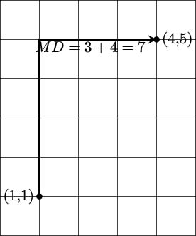
Here’s a two-dimensional sketch of the Euclidean distance between two points:

The Manhattan distance sums the edges of each leg of the right-angled triangle among the three points. It’s named after the gridded layout of the Borough of Manhattan in New York City. To get around, one is forced to travel only on the streets and avenues. Here’s the formal definition for three dimensions:
Here’s a two-dimensional sketch of the Manhattan distance between two points:
The Euclidean distance offers precision, while the Manhattan distance offers calculation speed.
Looking forward, we’re aiming for a structure that looks like this. For each individual pixel, we can compute the distance from that pixel’s color to the available colors in a limited color set. The results of this calculation for one individual pixel of an image might start like the following example:
[((0, 0),
  (92, 139, 195),
  Color(rgb=(239, 222, 205), name=’Almond’),
  169.10943202553784),
 ((0, 0),
  (92, 139, 195),
  Color(rgb=(255, 255, 153), name=’Canary’),
  204.42357985320578),
 ((0, 0),
  (92, 139, 195),
  Color(rgb=(28, 172, 120), name=’Green’),
  103.97114984456024),
 ((0, 0),
  (92, 139, 195),
  Color(rgb=(48, 186, 143), name=’Mountain Meadow’),
  82.75868534480233),
We’ve shown a sequence of tuples; each tuple has four items:
The pixel’s coordinates; for example, (0,0)
The pixel’s original color; for example, (92, 139, 195)
A
Colorobject from a set of seven colors; for example,Color(rgb=(48,186,143),name=’MountainMeadow’)The Euclidean distance between the original color and the given
Colorobject; for example, 82.75868534480233
It can help to create a NamedTuple to encapsulate the four items in each tuple. We could call it an X-Y, Pixel, Color, Distance tuple, something like ”XYPCD.” This would make it slightly easier to identify the (x,y) coordinate, the original pixel’s color, the matching color, and the distance between the original color and the selected match.
The smallest Euclidean distance is a closest match color. For the four example colors, the Mountain Meadow is the closest match for this pixel. This kind of reduction is done with the min() function. If the overall four-tuple of (x,y), pixel, color, and distance is assigned to a variable name, choices, the pixel-level reduction would look like this:
min(choices, key=lambda xypcd: xypcd[3])This expression will pick a single tuple as the optimal match between a pixel and color. It uses a lambda to select item 3 from the tuple, the distance metric.
9.2.2 Getting all pixels and all colors
How do we get to the structure that contains all pixels and all colors? One seemingly simple answer turns out to be less than optimal.
One way to map pixels to colors is to enumerate all pixels and all colors using the product() function:
from collections.abc import Iterable
from itertools import groupby

def matching_1(
        pixels: Iterable[Pixel],
        colors: Iterable[Color]
    ) -> Iterator[tuple[Point, RGB, Color, float]]:

    distances = (
        (pixel[0], pixel[1], color, euclidean(pixel[1], color))
        for pixel, color in product(pixels, colors)
    )
    for _, choices in groupby(distances, key=lambda xy_p_c_d: xy_p_c_d[0]):
        yield min(choices, key=lambda xypcd: xypcd[3])
The core of this is the product(pixel_iter(img), colors) expression that creates a sequence of all pixels combined with all colors. The overall expression then applies the euclidean() function to compute distances between pixels and Color objects. The result is a sequence of four-tuple objects with the original (x,y) coordinate, the original pixel, an available color, and the distance between the original pixel color and the available color.
The final selection of colors uses the groupby() function and the min(choices, ...) expression to locate the closest match.
The product() function applied to pixels and colors creates a long, flat iterable. We grouped the iterable into smaller collections where the coordinates match. This will break the big iterable into smaller iterables of only the pool of colors associated with a single pixel. We can then pick the minimal color distance for each available color for a pixel.
In a picture that’s 3,648×2,736 pixels with 133 Crayola colors, we have an iterable with 3,648 × 2,736 × 133 = 1,327,463,424 items to be evaluated. That is a billion combinations created by this distances expression. The number is not necessarily impractical; it’s well within the limits of what Python can do. However, it reveals an important flaw in the naive use of the product() function.
We can’t trivially do this kind of large-scale processing without first doing some analysis to see how large the intermediate data will be. Here are some timeit numbers for these two distance functions. This is the overall number of seconds to do each of these calculations only 1,000,000 times:
Euclidean: 1.761
Manhattan: 0.857
Scaling up by a factor of 1,000—from 1 million combinations to 1 billion—means the processing will take at least 1,800 seconds; that is, about half an hour for the Manhattan distance and 46 minutes to calculate the Euclidean distance. It appears this kind of naive bulk processing is ineffective for large datasets.
More importantly, we’re doing it wrong. This kind of width × height × color processing is simply a bad design. In many cases, we can do much better.
9.3 Performance improvements
A key feature of any big data algorithm is locating a way to execute some kind of a divide-and-conquer strategy. This is true of functional programming design as well as imperative design.
Here are three options to speed up this processing:
We can try to use parallelism to do more of the calculations concurrently. On a four-core processor, the time can be cut to approximately 25 percent. This reduces the time to 8 minutes for Manhattan distances.
We can see if caching intermediate results will reduce the amount of redundant calculation. The question arises of how many colors are the same and how many colors are unique.
We can look for a radical change in the algorithm.
We’ll combine the last two points by computing all the possible comparisons between source colors and target colors. In this case, as in many other contexts, we can easily enumerate the entire mapping of pixels and colors. If colors are repeated, we avoid doing redundant calculations to locate the closest color. We’ll also change the algorithm from a series of comparisons to a series of lookups in a mapping object.
In many problem domains, the source data is a collection of floating-point values. While these float values are flexible, and correspond in some ways with the mathematical abstraction of real numbers, they introduce some additional costs. Float operations can be slower than integer operations. More importantly, float values can contain a number of ”noise” bits. For example, common RGB color definitions use 256 distinct values for each of the Red, Green, and Blue components. These values are represented exactly with 8 bits. A floating-point variant, using values from 0.0 to 1.0, would use the full 64 bits for each color. Any arithmetic that led to floating-point truncation would introduce noise. While float values seem simple, they introduce troubling problems.
Here’s an example, using a red r=15:
>>> r = 15
>>> r_f = 15/256
>>> r_f
0.05859375
>>> r_f + 1/100 - 1/100
0.05859374999999999
Algebraically, rf + ![]() −
−![]() = rf. However, the
= rf. However, the float definition is only an approximation of the abstract concept of a real number. The value of ![]() doesn’t have an exact representation in binary-based floating-point. Using a value like this introduces truncation errors that propagate through subsequent computations. We’ve chosen to use integer-based color matching to show a way to minimize the additional complications that can arise from floating-point values.
doesn’t have an exact representation in binary-based floating-point. Using a value like this introduces truncation errors that propagate through subsequent computations. We’ve chosen to use integer-based color matching to show a way to minimize the additional complications that can arise from floating-point values.
When looking at this idea of pre-computing all transformations from source color to target color, we need some overall statistics for an arbitrary image. The code associated with this book includes IMG_2705.jpg. Here is a basic algorithm to collect all of the distinct color tuples from the specified image:
from collections import defaultdict, Counter
def gather_colors() -> defaultdict[RGB, list[Point]]:
    img = Image.open("IMG_2705.jpg")

    palette = defaultdict(list)
    for xy, rgb in pixel_iter(img):
        palette[rgb].append(xy)

    w, h = img.size
    print(f"total pixels {w*h}")
    print(f"total colors {len(palette)}")
    return palette
We collected all pixels of a given color into a list organized by color. From this, we’ll learn the following facts:
The total number of pixels is 9,980,928. This fits the expectation for a 10-megapixel image.
The total number of colors is 210,303. If we try to compute the Euclidean distance between actual colors and the 133 target colors, we would do 27,970,299 calculations, which might take about 76 seconds.
If we use a less accurate representation, one with fewer bits, we can speed things up. We’ll call this ”masking” to remove some of the irrelevant least-significant bits. Using a 3-bit mask,
0b11100000, the total number of colors actually used is reduced to 214 out of a domain of 23 × 23 × 23 = 512 possible colors.Using a 4-bit mask,
0b11110000, 1,150 colors are actually used.Using a 5-bit mask,
0b11111000, 5,845 colors are actually used.Using a 6-bit mask,
0b11111100, 27,726 colors are actually used. The domain of possible colors swells to 26 × 26 × 26 = 262,144.
This gives us some insight into how we can rearrange the data structure, calculate the matching colors quickly, and then rebuild the image without doing a billion comparisons and avoiding any additional complications from floating-point approximations. There are a number of changes required to avoid needless (and error-introducing) computations.
The core idea behind masking is to preserve the most significant bits of a value and eliminate the least significant bits. Consider a color with a red value of 200. We can use the Python bin() function to see the binary representation of that value:
>>> bin(200)
’0b11001000’
>>> 200 & 0b11100000
192
>>> bin(192)
’0b11000000’
The computation of 200 & 0b11100000 applied a mask to conceal the least significant 5 bits and preserve the most significant 3 bits. What remains after the mask is applied as a red value of 192.
We can apply mask values to the RGB three-tuple with the following command:
masked_color = tuple(map(lambda x: x & 0b11100000, c))This will pick out the most significant 3 bits of the red, green, and blue values of a color tuple by using the & operator to select particular bits from an integer value. If we use this masked value instead of the original color to create a Counter object, we’ll see that the image only uses 214 distinct values after the mask is applied. This is fewer than half the theoretical number of colors.
9.3.1 Rearranging the problem
The naive use of the product() function to compare all pixels and all colors was a bad idea. There are 10 million pixels, but only 200,000 unique colors. When mapping the source colors to target colors, we only have to save 200,000 values in a simple map.
We’ll approach it as follows:
Compute the source-to-target color mapping. In this case, let’s use 3-bit color values as output. Each R, G, and B value comes from the eight values in the
range(0,256,32)expression. We can use this expression to enumerate all the output colors:product(range(0, 256, 32), range(0, 256, 32), range(0, 256, 32))We can then compute the Euclidean distance to the nearest color in our source palette, doing just 68,096 calculations. This takes about 0.14 seconds. It’s done one time only and computes the 200,000 mappings.
In one pass through the source image, we build a new image using the revised color table. In some cases, we can exploit the truncation of integer values. We can use an expression such as
(0b11100000&r,0b11100000&g,0b11100000&b)to remove the least significant bits of an image color. We’ll look at this additional reduction in computation later.
This will replace a billion distance calculations with 10 million dictionary lookups, transforming a potential 30 minutes of calculation into about 30 seconds.
Given a source palette of approximately 200,000 colors, we can apply a fast Manhattan distance to locate the nearest color in a target palette, such as the Crayola colors.
We’ll fold in yet another optimization—truncation. This will give us an even faster algorithm.
9.3.2 Combining two transformations
When combining multiple transformations, we can build a more complex mapping from the source through intermediate targets to the result. To illustrate this, we’ll truncate the colors as well as applying a mapping.
In some problem contexts, truncation can be difficult. In other cases, it’s often quite simple. For example, truncating US postal ZIP codes from nine to five characters is common. Postal codes can be further truncated to three characters to determine a regional facility that represents a larger geography.
For colors, we can use the bit-masking shown previously to truncate colors from three 8-bit values (24 bits, 16 million colors) to three 3-bit values (9 bits, 512 colors).
Here is a way to build a color map that combines distances to a given set of colors and truncation of the source colors:
from collections.abc import Sequence
def make_color_map(colors: Sequence[Color]) -> dict[RGB, Color]:
    bit3 = range(0, 256, 0b0010_0000)

    best_iter = (
        min((euclidean(rgb, c), rgb, c) for c in colors)
        for rgb in product(bit3, bit3, bit3)
    )
    color_map = dict((b[1], b[2]) for b in best_iter)
    return color_map
We created a range object, bit3, that will iterate through all eight of the 3-bit color values. The use of the binary value, 0b0010_0000, can help visualize the way the bits are being used. The least significant 5 bits will be ignored; only the upper 3 bits will be used.
The range objects aren’t like ordinary iterators; they can be used multiple times. As a result of this, the product(bit3, bit3, bit3) expression will produce all 512 color combinations that we’ll use as the output colors.
For each truncated RGB color, we created a three-tuple that has (0) the distance from all crayon colors, (1) the RGB color, and (2) the crayon Color object. When we ask for the minimum value of this collection, we’ll get the closest crayon Color object to the truncated RGB color.
We built a dictionary that maps from the truncated RGB color to the closest crayon. In order to use this mapping, we’ll truncate a source color before looking up the nearest crayon in the mapping. This use of truncation coupled with the pre-computed mapping shows how we might need to combine mapping techniques.
The following function will build a new image from a color map:
def clone_picture(
    color_map: dict[RGB, Color],
    filename: str = "IMG_2705.jpg"
) -> None:
    mask = 0b1110_0000
    img = Image.open(filename)
    clone = img.copy()
    for xy, rgb in pixel_iter(img):
        r, g, b = rgb
        repl = color_map[(mask & r, mask & g, mask & b)]
        clone.putpixel(xy, repl.rgb)
    clone.show()
This uses the PIL putpixel() function to replace all of the pixels in a picture with other pixels. The mask value preserves the upper-most three bits of each color, reducing the number of colors to a subset.
What we’ve seen is that the naive use of some functional programming tools can lead to algorithms that are expressive and succinct, but also inefficient. The essential tools to compute the complexity of a calculation (sometimes called Big-O analysis) is just as important for functional programming as it is for imperative programming.
The problem is not that the product() function is inefficient. The problem is that we can use the product() function to create an inefficient algorithm.
9.4 Permuting a collection of values
When we permute a collection of values, we’ll generate all the possible orders for the values in the collection. There are n! permutations of n items. We can use a sequence of permutations as a kind of brute-force solution to a variety of optimization problems.
Typical combinatorial optimization problems are the Traveling Salesman problem, the Minimum Spanning Tree problem, and the Knapsack problem. These problems are famous because they involve potentially vast numbers of permutations. Approximate solutions are necessary to avoid exhaustive enumeration of all permutations. The use of the itertools.permutations() function is only handy for exploring very small problems.
One popular example of these combinatorial optimization problems is the assignment problem. We have n agents and n tasks, but the cost of each agent performing a given task is not equal. Imagine that some agents have trouble with some details, while other agents excel at these details. If we can properly assign tasks to agents, we can minimize the costs.
We can create a simple grid that shows how well a given agent is able to perform a given task. For a small problem of seven agents and tasks, there will be a grid of 49 costs. Each cell in the grid shows agents A0 to A6 performing tasks T0 to T6:
Task
A0
A1
A2
A3
A4
A5
A6
T0
14
11
6
20
12
9
4
T1
15
28
34
4
12
24
21
T2
16
31
22
18
31
15
23
T3
20
18
9
15
30
4
18
T4
24
8
24
30
28
25
4
T5
3
23
22
11
5
30
5
T6
13
7
5
10
7
7
32
Given this grid, we can enumerate all the possible permutations of agents and their tasks. However, this approach doesn’t scale well. For this problem, there are 720 alternatives. If we have more agents, for example 10, the value of 10! is 3,628,800. We can create the entire sequence of 3 million items with the list(permutations(range(10))) expression.
We would expect to solve a problem of this tiny size in a fraction of a second. For 10!, we might take a few seconds. When we double the size of the problem to 20!, we have a bit of a scalability problem: there will be 2.433 × 10¹⁸ permutations. On a computer where it takes about 0.56 seconds to generate 10! permutations, the process of generating 20! permutations would take about 12,000 years.
We can formulate the exhaustive search for the optimal solution as follows:
from itertools import permutations

def assignment(cost: list[tuple[int, ...]]) -> list[tuple[int, ...]]:
    n_tasks = len(cost)
    perms = permutations(range(n_tasks))
    alt = [
        (
            sum(
                cost[task][agent] for agent, task in enumerate(perm)
            ),
            perm
        )
        for perm in perms
    ]
    m = min(alt)[0]
    return [ans for s, ans in alt if s == m]
We’ve created all permutations of tasks for a group of agents and assigned this to perms. From this, we’ve created two-tuples of the sum of all costs in the cost matrix for a given permutation. To locate the relevant costs, a specific permutation is enumerated to create two-tuples showing the agent and the task assignment for that agent. For example, one of the permutations is tasks (2, 4, 6, 1, 5, 3, 0). We can assign agent index values using the expression list(enumerate((2, 4, 6, 1, 5, 3, 0))). The result, [(0, 2), (1, 4), (2, 6), (3, 1), (4, 5), (5, 3), (6, 0)], has all seven agent index values and their associated task assignments. We can translate the index numbers to agent names and task names by incorporating a dictionary lookup. The sum of the values in the cost matrix tells us how expensive this specific task assignment would be.
One of the optimal solutions might look like the assignment above. It requires folding in the agent names and task names to translate the task permutation into a specific list of assignments:
| A0 | T2 |
| A1 | T4 |
| A2 | T6 |
| A3 | T1 |
| A4 | T5 |
| A5 | T3 |
| A6 | T0 |
In some cases, there might be multiple optimal solutions; this algorithm will locate all of them. The expression min(alt)[0] selects the first of the set of minima.
For small textbook examples, this seems to be reasonably fast. There are linear programming approaches which avoid exhaustive enumeration of all permutations. The Python Linear Programming module PuLP can be used to solve the assignment problem. See https://coin-or.github.io/pulp/.
9.5 Generating all combinations
The itertools module also supports computing all combinations of a set of values. When looking at combinations, the order doesn’t matter, so there are far fewer combinations than permutations. The number of combinations is often stated as ![]() =
= ![]() . This is the number of ways that we can take combinations of r things at a time from a universe of p items overall.
. This is the number of ways that we can take combinations of r things at a time from a universe of p items overall.
For example, there are 2,598,960 five-card poker hands. We can actually enumerate all 2 million hands by executing the following command:
>>> from itertools import combinations, product

>>> hands = list(
...     combinations(
...         tuple(
...             product(range(13), ’♠♡♢♣’)
...         ), 5
...     )
... )
More practically, assume we have a dataset with a number of variables. A common exploratory technique is to determine the correlation among all pairs of variables in a set of data. If there are v variables, then we will enumerate all variables that must be compared by executing the following command:
>>> combinations(range(v), 2)A fun source of data for simple statistical analysis is the Spurious Correlations site. This has a great many datasets with surprising statistical properties. Let’s get some sample data from Spurious Correlations, http://www.tylervigen.com, to show how this will work. We’ll pick three datasets with the same time range, datasets numbered 7, 43, and 3,890. We’ll simply catenate the data into a grid. Because the source data repeats the year column, we’ll start with data that includes the repeated year column. We’ll eventually remove the obvious redundancy, but it’s often best to start with all of the data present as a way to confirm that the various sources of data align with each other properly.
This is how the first and the remaining rows of the yearly data will look:
[(’year’, ’Per capita consumption of cheese (US)Pounds (USDA)’,
’Number of people who died by becoming tangled in their
bedsheets Deaths (US) (CDC)’,
’year’, ’Per capita consumption of mozzarella cheese (US)Pounds
(USDA)’, ’Civil engineering doctorates awarded (US) Degrees awarded
(National Science Foundation)’,
’year’, ’US crude oil imports from Venezuela Millions of barrels
(Dept. of Energy)’, ’Per capita consumption of high fructose corn
syrup (US) Pounds (USDA)’),

(2000, 29.8, 327, 2000, 9.3, 480, 2000, 446, 62.6),
(2001, 30.1, 456, 2001, 9.7, 501, 2001, 471, 62.5),
(2002, 30.5, 509, 2002, 9.7, 540, 2002, 438, 62.8),
(2003, 30.6, 497, 2003, 9.7, 552, 2003, 436, 60.9),
(2004, 31.3, 596, 2004, 9.9, 547, 2004, 473, 59.8),
(2005, 31.7, 573, 2005, 10.2, 622, 2005, 449, 59.1),
(2006, 32.6, 661, 2006, 10.5, 655, 2006, 416, 58.2),
(2007, 33.1, 741, 2007, 11, 701, 2007, 420, 56.1),
(2008, 32.7, 809, 2008, 10.6, 712, 2008, 381, 53),
(2009, 32.8, 717, 2009, 10.6, 708, 2009, 352, 50.1)]
This is how we can use the combinations() function to yield all the combinations of the nine variables in this dataset, taken two at a time:
>>> combinations(range(9), 2)There are 36 possible combinations. We’ll have to reject the combinations that involve matching columns year and year. These will trivially correlate with a value of 1.00.
Here is a function that picks a column of data out of our dataset:
from typing import TypeVar
from collections.abc import Iterator, Iterable
T = TypeVar("T")

def column(source: Iterable[list[T]], x: int) -> Iterator[T]:
    for row in source:
        yield row[x]
This allows us to use the corr() function from Chapter 4, Working with Collections, to compute the correlation between the two columns of data.
This is how we can compute all combinations of correlations:
from collections.abc import Iterator
from itertools import *
from Chapter04.ch04_ex4 import corr

def multi_corr(
        source: list[list[float]]
    ) -> Iterator[tuple[float, float, float]]:
    n = len(source[0])
    for p, q in combinations(range(n), 2):
        header_p, *data_p = list(column(source, p))
        header_q, *data_q = list(column(source, q))
        if header_p == header_q:
            continue
        r_pq = corr(data_p, data_q)
        yield header_p, header_q, r_pq
For each combination of columns, we’ve extracted the two columns of data from our dataset. The header_p, *data_p =... statement uses multiple assignments to separate the first item in the sequence, the header, from the remaining rows of data. If the headers match, we’re comparing a variable to itself. This will be True for the three combinations of year and year that stem from the redundant year columns.
Given a combination of columns, we will compute the correlation function and then print the two headings along with the correlation of the columns. We’ve intentionally chosen two datasets that show spurious correlations with a third dataset that does not follow the same pattern as closely. In spite of this, the correlations are remarkably high.
The results look like this:
0.96: year vs Per capita consumption of cheese (US) Pounds (USDA)

0.95: year vs Number of people who died by becoming tangled in their
bedsheets Deaths (US) (CDC)

0.92: year vs Per capita consumption of mozzarella cheese (US) Pounds
(USDA)

0.98: year vs Civil engineering doctorates awarded (US) Degrees awarded
(National Science Foundation)

-0.80: year vs US crude oil imports from Venezuela Millions of barrels
(Dept. of Energy)

-0.95: year vs Per capita consumption of high fructose corn syrup (US)
Pounds (USDA)

0.95: Per capita consumption of cheese (US) Pounds (USDA) vs Number of
people who died by becoming tangled in their bedsheets Deaths (US) (CDC)

0.96: Per capita consumption of cheese (US)Pounds (USDA) vs year

0.98: Per capita consumption of cheese (US)Pounds (USDA) vs Per capita
consumption of mozzarella cheese (US)Pounds (USDA)

...

0.88: US crude oil imports from Venezuela Millions of barrels (Dept. of
Energy) vs Per capita consumption of high fructose corn syrup (US)Pounds
(USDA)
It’s not at all clear what this pattern means. Why do these values correlate? The presence of spurious correlations with no significance can cloud statistical analysis. We’ve located data that has strangely high correlations with no obvious causal factors.
What’s important is that a simple expression, combinations(range(9), 2), enumerates all the possible combinations of data. This kind of succinct, expressive technique makes it easier to focus on the data analysis issues instead of the combinatoric algorithm considerations.
9.5.1 Combinations with replacement
The itertools library has two functions for generating combinations of items selected from some set of values. The combinations() function reflects our expectations when dealing hands from a deck of cards: each card will appear at most once. The combinations_with_ replacement() function reflects the idea of taking a card from a deck, writing it down, and then shuffling it back into the deck before selecting another card. This second procedure could potentially yield a five-card sample with five aces of spades.
We can see this more clearly by using the following kind of expression:
>>> import itertools
>>> from pprint import pprint
>>> pprint(
... list(itertools.combinations([1,2,3,4,5,6], 2))
... )
[(1, 2),
 (1, 3),
 (1, 4),
...
 (4, 6),
 (5, 6)]
>>> pprint(
... list(itertools.combinations_with_replacement([1,2,3,4,5,6], 2))
... )
[(1, 1),
 (1, 2),
 (1, 3),
...
 (5, 5),
 (5, 6),
 (6, 6)]
There are ![]() = 15 combinations of six things taken two at a time. There are 62 = 36 combinations when replacement is permitted, since any value is a possible member of the result.
= 15 combinations of six things taken two at a time. There are 62 = 36 combinations when replacement is permitted, since any value is a possible member of the result.
9.6 Recipes
The itertools chapter of the Python library documentation is outstanding. The basic definitions are followed by a series of recipes that are extremely clear and helpful. Since there’s no reason to reproduce these, we’ll reference them here. They are required reading materials on functional programming in Python.
The Itertools Recipes section in the Python Standard Library is a wonderful resource. Visit https://docs.python.org/3/library/itertools.html#itertools-recipes for more details.
These function definitions aren’t importable functions in the itertools modules. These are ideas that need to be read and understood and then, perhaps, copied or modified before inclusion in an application.
The following table summarizes some recipes that show functional programming algorithms built from the itertools basics:
Function Name | Arguments | Results |
|
| Generate all the subsets of the iterable. Each subset is a tuple object, not a set instance. |
|
| Randomly select from |
|
| Randomly select from |
|
| Randomly select from |
9.7 Summary
In this chapter, we looked at a number of functions in the itertools module. This standard library module provides a number of functions that help us work with iterators in sophisticated ways.
We looked at these combination-producing functions:
The
product()function computes all the possible combinations of the elements chosen from two or more collections.The
permutations()function gives us different ways to reorder a given set of values.The
combinations()function returns all the possible subsets of an original set.
We also looked at ways in which the product() and permutations() functions can be used naively to create extremely large result sets. This is an important cautionary note. A succinct and expressive algorithm can also involve a vast amount of computation. We must perform basic complexity analysis to be sure that the code will finish in a reasonable amount of time.
In the next chapter, we’ll look at the functools module. This module includes some tools to work with functions as first-class objects. This builds on some material shown in Chapter 2, Introducing Essential Functional Concepts, and Chapter 5, Higher-Order Functions.
9.8 Exercises
This chapter’s exercises are based on code available from Packt Publishing on GitHub. See https://github.com/PacktPublishing/Functional-Python-Programming-3rd-Edition.
In some cases, the reader will notice that the code provided on GitHub includes partial solutions to some of the exercises. These serve as hints, allowing the reader to explore alternative solutions.
In many cases, exercises will need unit test cases to confirm they actually solve the problem. These are often identical to the unit test cases already provided in the GitHub repository. The reader should replace the book’s example function name with their own solution to confirm that it works.
9.8.1 Alternative distance computations
See Effects of Distance Measure Choice on KNN Classifier Performance - A Review. This is available at https://arxiv.org/pdf/1708.04321. In this paper, dozens of distance metrics are examined for their utility in implementing the k-Nearest Neighbors (k-NN) classifier.
Some of these are also suitable for the color-matching algorithm presented in this chapter. We defined a color, c, a three-tuple, (r,g,b), based on the Red, Green, and Blue components of the color. We can compute the distance between two colors, D(c1,c2), based on their RGB components:
We showed two: Euclidean and Manhattan distances. Here are some more formal definitions:
Some additional examples include these:
The Chebyshev Distance (CD) is the maximum of the absolute values of each color difference:

The Sorensen Distance (SD) is a modification of the Manhattan distance that tends to normalize the distance:

Redefine the make_color_map() function to be a higher-order function that will accept a distance function as a parameter. All of the distance functions should have a type hint of Callable[[RGB, Color], float]. Once the make_color_map() function has been changed, it becomes possible to create alternative color maps with alternative distance functions.
This function creates a mapping from ”masked” RGB values to a defined set of colors. Using a 3-bit mask defines a mapping from 23 × 23 × 23 = 512 possible RGB values to the domain of 133 colors.
The function’s definition should look like this:
def make_color_map(colors: Sequence[Color], distance: Callable[[RGB, Color], float]) -> dict[RGB, Color]:How much difference does the choice of distance function make? How can we characterize the mapping from the large collection of possible RGB values to the limited domain of subset colors? Is a histogram showing how many distinct RGB values map to a subset color sensible and informative?
9.8.2 Actual domain of pixel color values
When creating a color map, a mask was used to reduce the domain of possible colors from 28 × 28 × 28 = 16,777,216 to a more manageable 23 × 23 × 23 = 512 possible values.
Does it make sense to scan the original image using the mask value to determine the actual domain of available colors? A given image, may, for example, have only 210 distinct colors when a 3-bit mask is used. How much additional time is required to create this summary of colors actually in use?
Can the color summary be further optimized? Could we, for example, exclude rarely used colors? If we do exclude these rarely used colors, how do we replace a pixel’s color with more commonly used colors? What changes in an image if we use the color of the majority of the neighboring pixels to replace pixels with rarely used colors?
Consider an algorithm that makes the following two passes over an image’s pixels:
Create a
Counterwith the frequency of each color.For colors with fewer than some threshold, ?, locate the neighboring pixels. In a corner, there may be as few as three. In the middle, there will be no more than eight. Find the color of the majority of those pixels and replace the outlier.
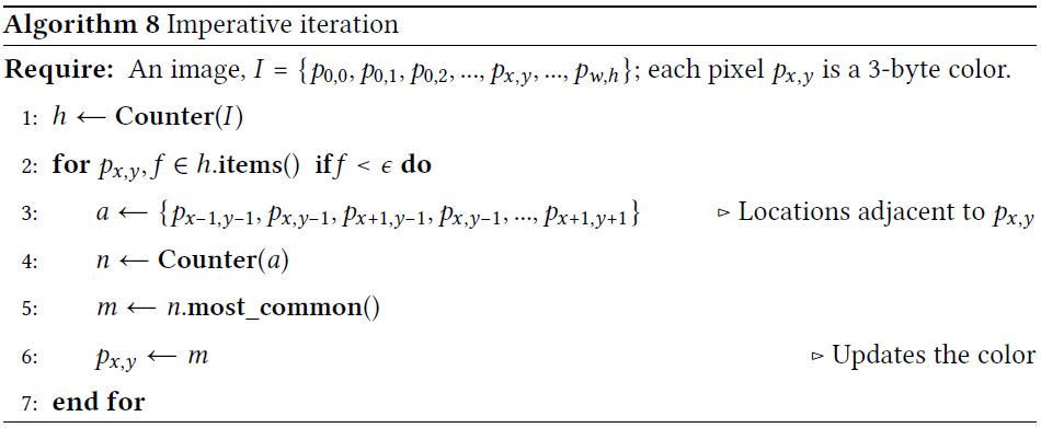
Before starting on this algorithm, it’s important to consider any ”edge” cases. Specifically, there is a potential complication when rarely used colors are adjacent.
Consider this case:
| p(0,0) | p(1,0) | p(2,0) |
| p(0,1) | p(1,1) | p(2,1) |
| p(0,2) | p(1,2) | p(2,2) |
If the four pixels in the top-left corner, p(0,0), p(1,0), p(0,1), and p(1,1), all had rarely used colors, then it would be difficult to pick a majority color to replace p(0,0).
In the case where there are no non-rare colors surrounding a pixel with a rare color, the algorithm would need to queue this up for later resolution after the neighbors have been processed. In this example, the color for pixel p(1,0) can be computed using neighbors that are not rare colors. After p(0,1) and p(1,1) are also resolved, then p(0,0) can be replaced with the majority color of the three neighbors.
Is this algorithmic complexity helpful for a picture with 10 million pixels? Choosing one or a few photos arbitrarily isn’t a sophisticated survey. However, it can help to avoid overthinking potential problems.
Survey the colors in a collection of images. How common is it to see a single pixel with a unique color? If you don’t have a private collection of images, visit kaggle.com to look for image datasets that can be examined.
9.8.3 Cribbage hand scoring
The card game of cribbage involves a phase where a player’s hand is evaluated. A player will use four cards that are dealt to them, plus a fifth card, called the starter.
To avoid overusing the word ”points,” we’ll consider each card to have a number of pips. Each face card is counted as having 10 pips; all other cards have a number of pips equal to their rank. Aces have a single pip.
The scoring involves the following combinations of cards:
Any combination of cards that totals 15 pips adds 2 points to the score.
Pairs – two cards of the same rank – add 2 points to the score.
Any run of three, four, or five cards adds 3, 4, or 5 points to the score.
A flush of four cards in a hand adds 4 points to the score. If the starter card is of the same suit, then the flush, as a whole, is 5 points.
If a jack in a hand has the same suit as the starter card, this adds 1 point to the score.
If a hand contains three cards of the same rank, this is counted as three separate pairs, worth 6 points in aggregate.
An interesting hand involves runs with a pair. For example, a hand 7C, 7D, 8H, and 9S, with an irrelevant starter card of a Queen, has two runs—7C, 8H, 9S, and 7D, 8H, 9S—and a pair of 7’s. This is a total of 8 points. Furthermore, there are two combinations that add to 15: 7C, 8H and 7D, 8H, bringing the hand’s value to 12 points.
Note that a 4-card run is not counted as two overlapping 3-card runs. It’s only worth 4 points.
Another interesting example is holding 4C, 5D, 5H, 6S, and the starter card is 3C. There are two distinct runs of 4 cards: 3C, 4C, 5D, 6S, and 3C, 4C, 5H, 6S, as well a pair of 5s, leading to 10 points for this pattern. Additionally, there are two distinct ways to count 15 pips: 4C, 5D, 6S and 4C, 5H, 6S, adding 4 more points to the score.
A handy algorithm for this is to enumerate several combinations and permutations of cards to locate all the scoring. The following rules can be applied:
Iterate over the powerset of the cards. This is the set of all subsets: all of the singletons, all of the pairs, all of the triples, etc., up to the set of all five cards. Each of these is a distinct set, some of which will tally to 15 pips. For more information on generating the powerset, see the Itertools Recipes section of the Python Standard Library documentation.
Enumerate all pairs of cards to compute scores for any pairs. The
combinations()function works well for this.For sets of five cards, if they’re adjacent, ascending values, this is a run. If they’re not adjacent, ascending values, then enumerate the sets of four-card runs to see if either of these have adjacent numbers. Failing that test, enumerate all sets of three-card runs to see if any of these have adjacent numbers. The longest run applies to the score, and shorter runs are ignored.
Check the hand and starter for a five-flush. If there’s no five-flush, check the hand only for a four-flush. Only one of these two combinations is scored.
Also, check to see if the hand has a jack of the same suit as the starter.
Since there are only five cards involved in this, the number of permutations and combinations is rather small. Be prepared to summarize exactly how many combinations and permutations are required for a five-card hand.
Join our community Discord space
Join our Python Discord workspace to discuss and know more about the book: https://packt.link/dHrHU
