7
Complex Stateless Objects
Many of the examples we’ve looked at have either been functions using atomic (or scalar) objects, or relatively simple structures built from small tuples. We can often exploit Python’s immutable typing.NamedTuple as a way to build complex data structures. The class-like syntax seems much easier to read than the older collections.namedtuple syntax.
One of the beneficial features of object-oriented programming is the ability to create complex data structures incrementally. In some respects, an object can be viewed as a cache for results of functions; this will often fit well with functional design patterns. In other cases, the object paradigm provides for property methods that include sophisticated calculations to derive data from an object’s properties. Using properties of an otherwise immutable class is also a good fit for functional design ideas.
In this chapter, we’ll look at the following:
How we create and use
NamedTupleand frozen@dataclassdefinitions.Ways that immutable
NamedTupleor frozen@dataclassobjects can be used instead of stateful object classes.How to use the popular third-party
pyrsistentpackage instead of stateful object classes. This is not part of the standard library, and requires a separate install.Some techniques to write generic functions outside any polymorphic class definition. While we can rely on callable classes to create a polymorphic class hierarchy, in some cases, this might be a needless overhead in a functional design. This will touch on using the
matchstatement for identifying types or structures.
While frozen dataclasses and NamedTuple subclasses are nearly equivalent, a frozen dataclass omits the sequence features that a NamedTuple includes. Iterating over the members of a NamedTuple object is a confusing feature; a dataclass doesn’t suffer from this potential problem.
We’ll start our journey by looking at using NamedTuple subclasses.
7.1 Using tuples to collect data
In Chapter 3, Functions, Iterators, and Generators, we showed two common techniques to work with tuples. We’ve also hinted at a third way to handle complex structures. We can go with any of the following techniques, depending on the circumstances:
Use lambdas (or functions created with the
defstatement) to select a named item based on the indexUse lambdas (or
deffunctions) with multiple positional parameters coupled with*argsto assign a tuple of items to parameter namesUse a
NamedTupleclass to select an item by attribute name or index
Our trip data, introduced in Chapter 4, Working with Collections, has a rather complex structure. The data started as an ordinary time series of position reports. To compute the distances covered, we transposed the data into a sequence of legs with a start position, end position, and distance as a nested three-tuple.
Each item in the sequence of legs looks as follows as a three-tuple:
>>> some_leg = (
... (37.549016, -76.330295),
... (37.840832, -76.273834),
... 17.7246
... )
The first two items are the starting and ending points. The third item is the distance between the points. This is a short trip between two points on the Chesapeake Bay.
A nested tuple of tuples can be rather difficult to read; for example, expressions such as some_leg[0][0] aren’t very informative.
Let’s look at the three alternatives for selecting values out of a tuple. The first technique involves defining some simple selection functions that can pick items from a tuple by index position:
>>> start = lambda leg: leg[0]
>>> end = lambda leg: leg[1]
>>> distance = lambda leg: leg[2]

>>> latitude = lambda pt: pt[0]
>>> longitude = lambda pt: pt[1]
With these definitions, we can use latitude(start(some_leg)) to refer to a specific piece of data. It looks like this code example:
>>> latitude(start(some_leg))
37.549016
It’s awkward to provide type hints for lambdas. The following shows how this becomes complex-looking:
from collections.abc import Callable
from typing import TypeAlias

Point: TypeAlias = tuple[float, float]
Leg: TypeAlias = tuple[Point, Point, float]

start: Callable[[Leg], Point] = lambda leg: leg[0]
The type hint must be provided as part of the assignment statement. This tells mypy that the object named start is a callable function that accepts a single parameter of a type named Leg and returns a result of the Point type. A function created with the def statement will usually have an easier-to-read type hint.
A variation on this first technique for collecting complex data uses the *parameter notation to conceal some details of the index positions. The following are some selection functions that are evaluated with the * notation:
>>> start_s = lambda start, end, distance: start
>>> end_s = lambda start, end, distance: end
>>> distance_s = lambda start, end, distance: distance

>>> latitude_s = lambda lat, lon: lat
>>> longitude_s = lambda lat, lon: lon
With these definitions, we can extract specific pieces of data from a tuple. We’ve used the _s suffix to emphasize the need to use star, *, when evaluating these lambdas. It looks like this code example:
>>> longitude_s(*start_s(*some_leg))
-76.330295
This has the advantage of a little more clarity in the function definitions. The association between position and name is given by the list of parameter names. It can look a little odd to see the * operator in front of the tuple arguments to these selection functions. This operator is useful because it maps each item in a tuple to a parameter of the function.
While these are very functional, the syntax for selecting individual attributes can be confusing. Python offers two object-oriented alternatives, NamedTuple and the frozen @dataclass.
7.2 Using NamedTuple to collect data
The second technique for collecting data into a complex structure is typing.NamedTuple. The idea is to create a class that is an immutable tuple with named attributes. There are two variations available:
The
namedtuplefunction in thecollectionsmodule.The
NamedTuplebase class in thetypingmodule. We’ll use this almost exclusively because it allows explicit type hinting.
In the following examples, we’ll use nested NamedTuple classes such as the following:
from typing import NamedTuple

class PointNT(NamedTuple):
    latitude: float
    longitude: float

class LegNT(NamedTuple):
    start: PointNT
    end: PointNT
    distance: float
This changes the data structure from simple anonymous tuples to named tuples with type hints provided for each attribute. Here’s an example:
>>> first_leg = LegNT(
...     PointNT(29.050501, -80.651169),
...     PointNT(27.186001, -80.139503),
...     115.1751)
>>> first_leg.start.latitude
29.050501
The first_leg object was built as the LegNT subclass of the NamedTuple class. This object contains two other named tuple objects and a float value. Using first_leg.start.latitude will fetch a particular piece of data from inside the tuple structure. The change from prefix function names to postfix attribute names can be seen as a helpful emphasis. It can also be seen as a confusing shift in the syntax.
The NT suffix in the names is not a recommended practice.
We’ve included the suffix in the book to emphatically distinguish among similar-looking solutions to the problem of defining a useful class.
In actual applications, we’d choose one definition, and use the simplest, clearest names possible, avoiding needless suffixes that clutter up textbooks like this one.
Replacing simple tuple() functions with appropriate LegNT() or PointNT() function calls is important. This changes the processing that builds the data structure. It provides an explicitly named structure with type hints that can be checked by the mypy tool.
For example, take a look at the following code snippet to create point pairs from source data:
from collections.abc import Iterable, Iterator
from Chapter04.ch04_ex1 import pick_lat_lon

def float_lat_lon_tuple(
        row_iter: Iterable[list[str]]
) -> Iterator[tuple[float, float]]:
    lat_lon_iter = (pick_lat_lon(*row) for row in row_iter)
    return (
        (float(lat), float(lon))
        for lat, lon in lat_lon_iter
    )
This requires an iterable object whose individual items are a list of strings. A CSV reader, or KML reader, can do this. The pick_lat_lon() function picks two values from the row. The generator expression applies the pick_lat_lon() function to the data source. The final generator expression creates a somewhat more useful two-tuple from the two string values.
The preceding code would be changed to the following code snippet to create Point objects:
from Chapter04.ch04_ex1 import pick_lat_lon
from typing import Iterable, Iterator

def float_lat_lon(
    row_iter: Iterable[list[str]]
) -> Iterator[PointNT]:
              #------
    lat_lon_iter = (pick_lat_lon(*row) for row in row_iter)
    return (
        PointNT(float(lat), float(lon))
        #------
        for lat, lon in lat_lon_iter
    )
The PointNT() constructor has been injected into the code. The data type that is returned is revised to be Iterator[PointNT]. It’s clear that this function builds Point objects instead of anonymous two-tuples of floating-point coordinates.
Similarly, we can introduce the following to build the complete trip of LegNT objects:
from collections.abc import Iterable, Iterator
from typing import cast, TextIO
import urllib.request
from Chapter04.ch04_ex1 import legs, haversine, row_iter_kml

source_url = "file:./Winter%202012-2013.kml"
def get_trip(url: str=source_url) -> list[LegNT]:
    with urllib.request.urlopen(url) as source:
        path_iter = float_lat_lon(row_iter_kml(source))
        pair_iter = legs(path_iter)
        trip_iter = (
            LegNT(start, end, round(haversine(start, end), 4))
            for start, end in pair_iter
        )
        trip = list(trip_iter)
    return trip
The processing is defined as a sequence of generator expressions, each one of which is lazy and operates on a single object. The path_iter object uses two generator functions, row_iter_kml() and float_lat_lon(), to read the rows from a KML file, pick fields, and convert them to Point objects. The pair_iter() object uses the legs() generator function to yield overlapping pairs of Point objects showing the start and end of each leg.
The trip_iter generator expression creates the final LegNT objects from pairs of Point objects. These generated objects are consumed by the list() function to create a single list of legs. The haversine() function from Chapter 4, Working with Collections, is used to compute the distance.
The rounding is applied in this function for two reasons. First, as a practical matter, 0.0001 nautical miles is about 20 cm (7 inches). Pragmatically, rounding to 0.001 nautical miles involves fewer digits that offer a false sense of precision. Second–and more important–it makes the unit testing more reliable across platforms if we avoid looking at all the digits of a floating-point number.
The final trip object is a sequence of LegNT instances. It will look as follows when we try to print it:
>>> source_url = "file:./Winter%202012-2013.kml"
>>> trip = get_trip(source_url)

>>> trip[0].start
PointNT(latitude=37.54901619777347, longitude=-76.33029518659048)
>>> trip[0].end
PointNT(latitude=37.840832, longitude=-76.273834)
>>> trip[0].distance
17.7246
It’s important to note that the haversine() function was written to use simple tuples. We’ve reused this function with a NamedTuple class instance. As we carefully preserved the order of the arguments, this small change in representation from anonymous tuple to named tuple was handled gracefully by Python.
Since this is a class definition, we can easily add methods and properties. This ability to add features to a NamedTuple makes them particularly useful for computing derived values. We can, for example, more directly implement the distance computation as part of the Point class, as shown in the following code:
import math

class PointE(NamedTuple):
    latitude: float
    longitude: float

    def distance(self, other: "PointE", R: float = 360*60/math.tau) -> float:
        """Equirectangular, ’flat-earth’ distance."""
        Δϕ = (
            math.radians(self.latitude) - math.radians(other.latitude)
        )
        Δλ = (
            math.radians(self.longitude) - math.radians(other.longitude)
        )
        mid_ϕ = (
            (math.radians(self.latitude) - math.radians(other.latitude))
            / 2
        )
        x = R * Δλ * math.cos(mid_ϕ)
        y = R * Δϕ
        return math.hypot(x, y)
Given this definition of the PointE class, we have encapsulated the functions for working with points and distances. This can be helpful because it gives the reader a single place to look for the relevant attributes and methods.
Within the body of the PointE class, we can’t easily refer to the class. The class name doesn’t exist within the body of the class statement. The mypy tool lets us use a string instead of a class name to resolve these rare cases when a class needs to refer to itself.
We can use this class as shown in the following example:
>>> start = PointE(latitude=38.330166, longitude=-76.458504)
>>> end = PointE(latitude=38.976334, longitude=-76.473503)

# Apply the distance() method of the start object...
>>> leg = LegNT(start, end, round(start.distance(end), 4))
>>> leg.start == start
True
>>> leg.end == end
True
>>> leg.distance
38.7805
In most cases, the NamedTuple class definition adds clarity. The use of NamedTuple will lead to a change from function-like prefix syntax to object-like suffix syntax.
7.3 Using frozen dataclasses to collect data
The third technique for collecting data into a complex structure is the frozen @dataclass. The idea is to create a class that is an immutable collection of named attributes.
Following the example from the previous section, we can have nested dataclasses such as the following:
from dataclasses import dataclass

@dataclass(frozen=True)
class PointDC:
    latitude: float
    longitude: float

@dataclass(frozen=True)
class LegDC:
    start: PointDC
    end: PointDC
    distance: float
We’ve used a decorator, @dataclass(frozen=True), in front of the class definition to create an immutable (known as ”frozen”) dataclass. The decorator will add a number of functions for us, building a fairly sophisticated class definition without our having to provide anything other than the attributes. For more information on decorators, see Chapter 12, Decorator Design Techniques.
This also changes the data structure from simple anonymous tuples to a class definition with type hints provided for each attribute. Here’s an example:
>>> first_leg = LegDC(
...     PointDC(29.050501, -80.651169),
...     PointDC(27.186001, -80.139503),
...     115.1751)
>>> first_leg.start.latitude
29.050501
The first_leg object was built as the LegDC instance. This object contains two other PointDC objects and a float value. Using first_leg.start.latitude will fetch a particular attribute of the object.
The DC suffix in the names is not a recommended practice.
We’ve included the suffix in the book to emphatically distinguish among similar-looking solutions to the problem of defining a useful class.
In actual applications, we’d choose one definition, and use the simplest, clearest names possible, avoiding needless suffixes that clutter up textbooks like this one.
Replacing a () tuple construction with appropriate LegDC() or PointDC() constructors builds a more sophisticated data structure than anonymous tuples. It provides an explicitly named structure with type hints that can be checked by the mypy tool.
Comparing frozen dataclasses with NamedTuple instances can lead to a ”Which is better?” discussion. There are a few tradeoffs here. Most notably, a NamedTuple object is extremely simple: it ties up relatively little memory and offers few methods. A dataclass, on the other hand, can have a great deal of built-in functionality, and can tie up more memory. We can manage this using the slots=True argument with the @dataclass decorator, something we’ll address later in this section.
Additionally, a NamedTuple object is a sequence of values. We can use an iterator over the tuple’s attributes, a processing option that seems to create nothing but confusion. Iterating over the values without using the names subverts the essential design concept of naming the members of the tuple.
A simple procedure for evaluating memory use is to create millions of instances of a class and see how much memory is allocated for the Python runtime. This works out best because Python object size involves a recursive walk through all of the associated objects, each of which has its own complex sizing computation. Generally, we only care about aggregate memory use for a large collection of objects, so it’s more effective to measure that directly.
Here is one class definition to support a script designed to evaluate the size of 1,000,000 NamedTuple objects:
from typing import NamedTuple

class LargeNT(NamedTuple):
  a: str
  b: int
  c: float
  d: complex
We can then define a function to create a million objects, assigning them to a variable, big_sequence. The function can then report the amount of memory allocated by the Python runtime. This function will involve some odd-looking overheads. The documentation for the getallocatedblocks() function advises us to clear the type cache with the sys._clear_type_cache() function and force garbage collection via the gc.collect() function to clean up the objects that are no longer referenced. These two steps should compact memory to the smallest size, and provide more repeatable reports on the use of storage by this sequence of objects.
The following function creates a million instances of a given type and displays the allocated memory:
from typing import Type, Any

def sizing(obj_type: Type[Any]) -> None:
    big_sequence = [
        obj_type(f"Hello, {i}", 42*i, 3.1415926*i, i+2j)
        for i in range(1_000_000)
    ]
    sys._clear_type_cache()
    gc.collect()
    print(f"{obj_type.__name__} {sys.getallocatedblocks()}")
    del big_sequence
Evaluating this function with different class definitions will reveal how much storage is occupied by 1,000,000 objects of that class. We can use sizing(LargeNT) to see the space taken up by a NamedTuple class.
We’ll need to define alternatives, of course. We can define a frozen dataclass. Additionally, we can use @dataclass(frozen=True, slots=True) to see what impact the use of __slots__ has on the object sizing. The bodies of the classes must all have the same attributes in the same order to simplify construction of the objects by the sizing() function.
The actual results are highly implementation-specific, but the author’s results on macOS Python 3.10.0 show the following:
| Class Kind | Blocks Allocated |
| LargeNT | 5,035,408 |
| LargeDC | 7,035,404 |
| LargeDC_Slots | 5,035,569 |
| Baseline | 35,425 |
This suggests that a @dataclass will use about 40% more memory than a NamedTuple or a @dataclass with slots=True.
This also suggests that a radically different design—one that uses iterators to avoid creating large in-memory collections—can use substantially less memory. What’s important is to have a correct solution in hand, and then explore alternative implementations to see which makes most effective use of the machine resources.
How to implement a complicated initialization is the most telling distinction among the various class definition approaches. We’ll look at that next.
7.4 Complicated object initialization and property computations
When working with data in unhelpful formats, it often becomes necessary to build Python objects from source data that has a different structure or different underlying object types. There are two overall ways to treat object creation:
It’s part of the application as a whole. Data should be decomposed by a parser and recomposed into useful Python objects. This is the approach we’ve taken in previous examples.
It’s part of the object’s class definition. Source data should be provided more or less in its raw form, and the class definition will perform the necessary conversions.
This distinction is never simple, nor crisp. Pragmatic considerations will identify the best approach for each unique case of building a Pythonic object from source data. The two examples that point to the distinct choices available are the following:
The
Pointclass: The syntax for geographic points is highly variable. A common approach is simple floating-point degree numbers. However, some sources provide degrees and minutes. Others might provide separate degrees, minutes, and seconds. Further, there are also Open Location Codes, which encode latitude and longitude. (See https://maps.google.com/pluscodes/ for more information.) All of these various parsers should not be part of the class.The
LegNT(orLegDC) class: The leg includes two points and a distance. The distance can be seeded as a simple value. It can also be computed as a property. A third choice is to use a sophisticated object builder. In effect, ourget_trip()function (defined in Using NamedTuple to collect data) has implicitly included an object builder forLegNTobjects.
Using LegNT(start, end, round(haversine(start, end), 4)) to create a LegNT instance isn’t wrong, but it makes a number of assumptions that need to be challenged. Here are some of the assumptions:
The application should always use
haversine()to compute distances.The application should always pre-compute the distance. This is often an optimization question. Computing a distance once and saving it is helpful if every leg’s distance will be examined. If distances are not always needed, it can be less expensive to compute the distance only when required.
We always want to create
LegNTinstances. We’ve already seen cases where we might want a@dataclassimplementation. In the next section, we’ll look at apyrsistent.PRecordimplementation.
One general way to encapsulate the construction of LegNT instances is to use a @classmethod to handle complex initialization. Additionally, a @dataclass provides some additional initialization techniques.
A slightly better way to define a NamedTuple initialization is shown in the following example:
from typing import NamedTuple

class EagerLeg(NamedTuple):
    start: Point
    end: Point
    distance: float

    @classmethod
    def create(cls, start: Point, end: Point) -> "EagerLeg":
        return cls(
            start=start,
            end=end,
            distance=round(haversine(start, end), 4)
        )
Compare the above definition, which eagerly computes the distance, with the following, which lazily computes the distance:
from typing import NamedTuple

class LazyLeg(NamedTuple):
    start: Point
    end: Point

    @property
    def distance(self) -> float:
        return round(haversine(self.start, self.end), 4)

    @classmethod
    def create(cls, start: Point, end: Point) -> "LazyLeg":
        return cls(
            start=start,
            end=end
        )
Both of these class definitions have an identical create() method. We can use EagerLeg.create(start, end) or LazyLeg.create(start, end) without breaking anything else in the application.
What’s most important is that the decision to compute values eagerly or lazily becomes a decision that we can alter at any time. We can replace these two definitions to see which has higher performance for our specific application’s needs. The distance computation, similarly, is now part of this class, making it easier to define a subclass to make a change to the application.
A dataclass offers a somewhat more complex and flexible interface for object construction: a __post_init__() method. This method is evaluated after the object’s fields have their values assigned, permitting eager calculation of derived values. This, however, can’t work for frozen dataclasses. The __post_init__() method can only be used for non-frozen dataclasses to eagerly compute additional values from the provided initialization values.
For dataclasses, as well as NamedTuple classes, a @classmethod creator is a good design pattern for doing initialization that involves eagerly computing attribute values.
As a final note on initialization, there are three different syntax forms for creating named tuple objects. Here are the three choices:
We can provide the values positionally. This works well when the order of the parameters is obvious. It looks like this:
LegNT(start, end, round(haversine(start, end), 4))We can unpack a sequence using the
*operator. This, too, requires the ordering of parameters be obvious. For example:PointNT(*map(float, pick_lat_lon(*row)))We can use explicit keyword assignment. This has the advantage of making the parameter names clear and avoids hidden assumptions about ordering. Here’s an example:
PointNT(longitude=float(row[0]), latitude=float(row[1]))
These examples show one way to package the initialization of complex objects. What’s important is to avoid state change in these objects. A complex initialization is done exactly once, providing a single, focused place to understand how the object’s state was established. For this reason, it’s imperative for the initialization to be expressive of the object’s purpose as well as flexible to permit change.
7.5 Using pyrsistent to collect data
In addition to Python’s NamedTuple and @dataclass definitions, we can also use the pyrsistent module to create more complex object instances. The huge advantage offered by the pyrsistent module is that the collections are immutable. Instead of updating in place, a change to a collection works through a general-purpose ”evolution” object that creates a new immutable object with the changed value. In effect, what appears to be a state-changing method is actually an operator creating a new object.
The following example shows how to import the pyrsistent module and create a mapping structure with names and values:
>>> import pyrsistent
>>> v = pyrsistent.pmap({"hello": 42, "world": 3.14159})
>>> v  # doctest: +SKIP
pmap({’hello’: 42, ’world’: 3.14159})
>>> v[’hello’]
42
>>> v[’world’]
3.14159
We can’t change the value of this object, but we can evolve an object v to a new object, v2. This object has the same starting values, but also includes a changed attribute value. It looks like this:
>>> v2 = v.set("another", 2.71828)
>>> v2    # doctest: +SKIP
pmap({’hello’: 42, ’world’: 3.14159, ’another’: 2.71828})
The original object, v, is immutable, and its value hasn’t changed:
>>> v    # doctest: +SKIP
pmap({’hello’: 42, ’world’: 3.14159})
It can help to think of this operation as having two parts. First, the original object is cloned. After the cloning, the changes are applied. In the above example, the set() method was used to provide a new key and value. We can create the evolution separately and apply it to an object to create a clone with changes applied. This seems ideal for an application where an audit history of changes is required.
Note that we had to prevent using two examples as unit test cases. This is because the order of the keys isn’t fixed. It’s easy to check that the keys and values match our expectations, but a simplistic comparison with a dictionary literal doesn’t always work.
The PRecord class is appropriate for defining complex objects. These objects are similar in some ways to a NamedTuple. We’ll revisit our waypoint and leg data model using PRecord instances. The definitions are given in the following example:
from pyrsistent import PRecord, field

class PointPR(PRecord):  # type: ignore [type-arg]
    latitude = field(type=float)
    longitude = field(type=float)

class LegPR(PRecord):  # type: ignore [type-arg]
    start = field(type=PointPR)
    end = field(type=PointPR)
    distance = field(type=float)
Each field definition uses the sophisticated field() function to build the definition of the attribute. In addition to a sequence of types, this function can specify an invariant condition that must be true for the values, an initial value, whether or not the field is mandatory, a factory function that builds appropriate values, and a function to serialize the value into a string.
The PR suffix in the names is not a recommended practice.
We’ve included the suffix in the book to emphatically distinguish among similar-looking solutions to the problem of defining a useful class.
In actual applications, we’d choose one definition, and use the simplest, clearest names possible, avoiding needless suffixes that clutter up textbooks like this one.
As an extension to these definitions, we could convert the point value into a more useful format using a serializer function. This requires some formatting details because there’s a slight difference in the way latitudes and longitudes are displayed. Latitudes include ”N” or ”S” and longitudes include ”E” or ”W”:
from math import isclose, modf

def to_dm(format: dict[str, str], point: float) -> str:
    """Use {"+": "N", "-": "S"} for latitude; {"+": "E", "-": "W"} for longitude."""
    sign = "-" if point < 0 else "+"
    ms, d = modf(abs(point))
    ms = 60 * ms
    # Handle the 59.999 case:
    if isclose(ms, 60, rel_tol=1e-5):
        ms = 0.0
        d += 1
    return f"{d:3.0f}{ms:.3f}’{format.get(sign, sign)}"
This function can be included as part of the field definition for the PointPR class; we must provide the function as the serializer= parameter of the field() factory:
from pyrsistent import PRecord, field

class PointPR_S(PRecord):  # type: ignore[type-arg]
    latitude = field(
        type=float,
        serializer=(
            lambda format, value:
                to_dm((format or {}) | {"+": "N", "-": "S"}, value)
        )
    )
    longitude = field(
        type=float,
        serializer=(
            lambda format, value:
                to_dm((format or {}) | {"+": "E", "-": "W"}, value)
        )
    )
This lets us print a point in a nicely formatted style:
>>> p = PointPR_S(latitude=32.842833333, longitude=-79.929166666)
>>> p.serialize()  # doctest: +SKIP
{’latitude’: " 32°50.570’N", ’longitude’: " 79°55.750’W"}
These definitions will provide nearly identical processing capabilities to the NamedTuple and @dataclass examples shown earlier. We can, however, leverage some additional features of the pyrsistent package to create PVector objects, which will be immutable sequences of waypoints in a trip. This requires a few small changes to previous applications.
The definition of the get_trip() function using pyrsistent can look like this:
from collections.abc import Iterable, Iterator
from typing import TextIO
import urllib.request
from Chapter04.ch04_ex1 import legs, haversine, row_iter_kml
from pyrsistent import pvector
from pyrsistent.typing import PVector

source_url = "file:./Winter%202012-2013.kml"
def get_trip_p(url: str=source_url) -> PVector[LegPR]:
    with urllib.request.urlopen(url) as source:
        path_iter = float_lat_lon(row_iter_kml(source))
        pair_iter = legs(path_iter)
        trip_iter = (
            LegPR(
                start=PointPR.create(start._asdict()),
                end=PointPR.create(end._asdict()),
                distance=round(haversine(start, end), 4))
            #--------------------------------------------
            for start, end in pair_iter
        )
        trip = pvector(trip_iter)
               #------
    return trip
The first change is relatively large. Instead of rewriting the float_lat_lon() function to return a PointPR object, we left this function alone. We used the PRecord.create() method to convert a dictionary into a PointPR instance. Given the two PointPR objects and the distance, we can create a LegPR object.
Earlier in this chapter, we showed a version of the legs() function that returned typing.NamedTuple instances with the raw data for each point along a leg. The _asdict() method of a NamedTuple will translate the tuple into a dictionary. The tuple’s attribute names will be keys in the dictionary. The transformation can be seen in the following example:
>>> p = PointNT(2, 3)
>>> p._asdict()
{’latitude’: 2, ’longitude’: 3}
This can then be provided to the PointPR.create() method to create a proper PointPR instance that will be used in the rest of the application. The initial PointNT object can be discarded, having served as a bridge between input parsing and building more useful Python objects. In the long run, it’s a good idea to revisit the underlying legs() function to rewrite it to work with pyrsistent record definitions.
Finally, instead of assembling a list from the iterator, we assembled a PVector instance, using the pvector() function. This has many of the same properties as the built-in list class, but is immutable. Any changes will create a clone of the object.
These high-performance, immutable collections are helpful ways to be sure an application behaves in a functional manner. The handy serialization into JSON-friendly notation makes these class definitions ideal for applications that make use of JSON. Web servers, in particular, can benefit from using these class definitions.
7.6 Avoiding stateful classes by using families of tuples
In several previous examples, we’ve shown the idea of wrap-unwrap design patterns that allow us to work with anonymous and named tuples. The point of this kind of design is to use immutable objects that wrap other immutable objects instead of mutable instance variables.
A common statistical measure of correlation between two sets of data is the Spearman’s rank correlation. This compares the rankings of two variables. Rather than trying to compare values, which might have different units of measure, we’ll compare the relative orders. For more information, visit: https://www.itl.nist.gov/div898/software/dataplot/refman2/auxillar/partraco.htm.
Computing the Spearman’s rank correlation requires assigning a rank value to each observation. It seems like we should be able to use enumerate(sorted()) to do this. Given two sets of possibly correlated data, we can transform each set into a sequence of rank values and compute a measure of correlation.
We’ll apply the wrap-unwrap design pattern to do this. We’ll wrap data items with their rank for the purposes of computing the correlation coefficient.
In Chapter 3, Functions, Iterators, and Generators, we showed how to parse a simple dataset. We’ll extract the four samples from that dataset as follows:
>>> from Chapter03.ch03_ex4 import (
... series, head_map_filter, row_iter)
>>> from pathlib import Path

>>> source_path = Path("Anscombe.txt")
>>> with source_path.open() as source:
...     data = list(head_map_filter(row_iter(source)))
The resulting collection of data has four different series of data combined in each row. A series() function was defined in Generators for lists, dicts, and sets, back in Chapter 3, Functions, Iterators, and Generators, to extract the pairs for a given series from the overall row.
The definition looked like this:
def series(
      n: int,
      row_iter: Iterable[list[SrcT]]
) -> Iterator[tuple[SrcT, SrcT]]:
The argument to this function is an iterable of some source type (usually a string). The result of this function is an iterable series of two-tuples from the source type. When working with CSV files, strings are the expectation. It’s much nicer for the result to be a named tuple.
Here’s a named tuple for each pair:
from typing import NamedTuple

class Pair(NamedTuple):
    x: float
    y: float
We’ll introduce a transformation to convert anonymous tuples into named tuples or dataclasses:
from collections.abc import Callable, Iterable
from typing import TypeAlias

RawPairIter: TypeAlias = Iterable[tuple[float, float]]

pairs: Callable[[RawPairIter], list[Pair]]
    = lambda source: list(Pair(*row) for row in source)
The RawPairIter type definition describes the intermediate output from the series() function. This function emits an iterable sequence of two-tuples. The pairs lambda object is a callable that expects an iterable and will produce a list of Pair named tuples or dataclass instances.
The following shows how the pairs() function and the series() function are used to create pairs from the original data:
>>> series_I = pairs(series(0, data))
>>> series_II = pairs(series(1, data))
>>> series_III = pairs(series(2, data))
>>> series_IV = pairs(series(3, data))
Each of these series is a list of Pair objects. Each Pair object has x and y attributes. The data looks as follows:
>>> from pprint import pprint

>>> pprint(series_I)
[Pair(x=10.0, y=8.04),
 Pair(x=8.0, y=6.95),
 ...
 Pair(x=5.0, y=5.68)]
We’ll break the rank ordering problem into two parts. First, we’ll look at a generic, higher-order function that we can use to assign ranks to any attribute. For example, it can rank a sample according to either the the x or y attribute value of a Pair object. Then, we’ll define a wrapper around the Pair object that includes the various rank order values.
So far, this seems like a place where we can wrap each pair, sort them into order, then use a function like enumerate() to assign ranks. It turns out that this approach isn’t really the proper algorithm for rank ordering.
While the essence of rank ordering is being able to sort the samples, there’s another important part of this. When two observations have the same value, they should get the same rank. The general rule is to average the positions of equal observations. The sequence [0.8, 1.2, 1.2, 2.3, 18] should have rank values of 1, 2.5, 2.5, 4, 5. The two ties with ranks of 2 and 3 have the midpoint value of 2.5 as their common rank.
A consequence of this is that we don’t really need to sort all of the data. We can, instead, create a dictionary with a given attribute value and all of the samples that share the attribute value. All these items have a common rank. Given this dictionary, the keys need to be processed in ascending order. For some collections of data, there may be significantly fewer keys than original sample objects being ranked.
The rank ordering function works in two passes:
First, it builds a dictionary listing samples with duplicate values. We can call this the
build_duplicates()phase.Second, it emits a sequence of values, in ranked order, with a mean rank order for the items with the same value. We can call this the
rank_output()phase.
The following function implements the two-phase ordering via two embedded functions:
from collections import defaultdict
from collections.abc import Callable, Iterator, Iterable, Hashable
from typing import NamedTuple, TypeVar, Any, Protocol, cast

BaseT = TypeVar("BaseT", int, str, float)
DataT = TypeVar("DataT")

def rank(
    data: Iterable[DataT],
    key: Callable[[DataT], BaseT]
) -> Iterator[tuple[float, DataT]]:

    def build_duplicates(
            duplicates: dict[BaseT, list[DataT]],
            data_iter: Iterator[DataT],
            key: Callable[[DataT], BaseT]
    ) -> dict[BaseT, list[DataT]]:
        for item in data_iter:
            duplicates[key(item)].append(item)
        return duplicates

    def rank_output(
            duplicates: dict[BaseT, list[DataT]],
            key_iter: Iterator[BaseT],
            base: int=0
    ) -> Iterator[tuple[float, DataT]]:
        for k in key_iter:
            dups = len(duplicates[k])
            for value in duplicates[k]:
                yield (base+1+base+dups)/2, value
            base += dups

    duplicates = build_duplicates(
        defaultdict(list), iter(data), key
    )
    return rank_output(
        duplicates,
        iter(sorted(duplicates.keys())),
        0
    )
As we can see, this rank ordering function has two internal functions to transform a list of samples to a list of two-tuples, each pair having the assigned rank and the original sample object.
To keep the data structure type hints simple, the base type of the sample tuple is defined as BaseT, which can be any of the string, integer, or float types. The essential ingredient here is a simple, hashable, and comparable object.
Similarly, the DataT type is any type for the raw samples; the claim is that it will be used consistently throughout the function, and it’s two internal functions. This is an intentionally vague claim, because any kind of NamedTuple, dataclass, or PRecord will work.
The build_duplicates() function works with a stateful object to build the dictionary that maps keys to values. This implementation relies on the tail-call optimization of a recursive algorithm. The arguments to build_duplicates() expose the internal state as argument values. A base case for a recursive definition is when data_iter is empty.
Similarly, the rank_output() function could be defined recursively to emit the original collection of values as two-tuples with the assigned rank values. What’s shown is an optimized version with two nested for statements. To make the rank value computation explicit, it includes the low end of the range (base+1), the high end of the range (base+dups), and computes the midpoint of these two values. If there is only a single duplicate, the rank value is (2*base+2)/2, which has the advantage of being a general solution, resulting in base+1, in spite of extra computations.
The dictionary of duplicates has the type hint of dict[BaseT, list[tuple[BaseT, ...]]], because it maps a sample attribute value, BaseT, to lists of the original data item type, tuple[BaseT, ...].
The following is how we can test this to be sure it works. The first example ranks individual values. The second example ranks a list of pairs, using a lambda to pick the key value from each pair:
>>> from pprint import pprint

>>> data_1 = [(0.8,), (1.2,), (1.2,), (2.3,), (18.,)]
>>> ranked_1 = list(rank(data_1, lambda row: row[0]))
>>> pprint(ranked_1)
[(1.0, (0.8,)), (2.5, (1.2,)), (2.5, (1.2,)), (4.0, (2.3,)), (5.0, (18.0,))]

>>> from random import shuffle
>>> shuffle(data_1)
>>> ranked_1s = list(rank(data_1, lambda row: row[0]))
>>> ranked_1s == ranked_1
True

>>> data_2 = [(2., 0.8), (3., 1.2), (5., 1.2), (7., 2.3), (11., 18.)]
>>> ranked_2 = list(rank(data_2, key=lambda x: x[1],))
>>> pprint(ranked_2)
[(1.0, (2.0, 0.8)),
 (2.5, (3.0, 1.2)),
 (2.5, (5.0, 1.2)),
 (4.0, (7.0, 2.3)),
 (5.0, (11.0, 18.0))]
The sample data included two identical values. The resulting ranks split positions 2 and 3 to assign position 2.5 to both values. This confirms that the function implements the common statistical practice for computing the Spearman’s rank-order correlation between two sets of values.
The rank() function involves rearranging the input data as part of discovering duplicated values. If we want to rank on both the x and y values in each pair, we need to reorder the data twice.
7.6.1 Computing Spearman’s rank-order correlation
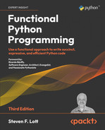
The Spearman rank-order correlation is a comparison between the rankings of two variables. It neatly bypasses the magnitude of the values, and it can often find a correlation even when the relationship is not linear. The formula is as follows:
This formula shows us that we’ll be summing the differences in rank rx, and ry, for all of the pairs of observed values. This requires computing ranks on both x and y variables. This means merging the two rank values into a single, composite object with ranking combined with the original raw sample.
The target class could look like the following:
class Ranked_XY(NamedTuple):
    r_x: float
    r_y: float
    raw: Pair
This can be built by first ranking on one variable, then computing a second ranking of the raw data. For a simple dataset with a few variables, this isn’t terrible. For more than a few variables, this becomes needlessly complicated. The function definitions, in particular for ranking, would all be nearly identical, suggesting a need to factor out the common code.
It works out much better to depend on using the pyrsistent module to create, and evolve, the values in a dictionary that accumulate ranking values. We can use a PRecord pair that has a dictionary of rankings and the original data. The dictionary of rankings is an immutable PMap. This means that any attempt to make a change will lead to evolving a new instance.
The instance, after being evolved, is immutable. We can clearly separate the accumulation of state from processing objects that do not have any further state changes.
Here’s our PRecord subclass that contains the ranking mapping and the original, raw data:
from pyrsistent import PRecord, field, PMap, pmap

class Ranked_XY(PRecord):  # type: ignore [type-arg]
    rank = field(type=PMap)
    raw = field(type=Pair)
Within each Ranked_XY, the PMap dictionary provides a mapping from the variable name to the ranking value. The raw data is the original sample. We want to be able to use sample.rank[attribute_name] to extract the ranking for a specific attribute.
We can reuse our generic rank() function to build the essential information that contains a ranking and the raw data. We can then merge each new ranking into a Ranked_XY instance. The following function definition will compute rankings for two attributes:
def rank_xy(pairs: Sequence[Pair]) -> Iterator[Ranked_XY]:
    data = list(Ranked_XY(rank=pmap(), raw=p) for p in pairs)

    for attribute_name in (’x’, ’y’):
        ranked = rank(
            data,
            lambda rxy: cast(float, getattr(rxy.raw, attribute_name))
        )
        data = list(
            original.set(
                rank=original.rank.set(attribute_name, r)  # type: ignore [arg-type]
            )
            for r, original in ranked
        )

    yield from iter(data)
We’ve built an initial list of Ranked_XY objects with empty ranking dictionaries. For each attribute of interest, we’ll use the previously defined rank() function to create a sequence of rank values and raw objects. The for clause of the generator decomposes the ranking two-tuple into r, the ranking, and original, the raw source data.
From each pair of values from the underlying rank() function, we’ve made two changes to the pyrsistent module’s data structures. We’ve used the following expression to create a new dictionary of the previous rankings merged with this new ranking:
original.rank.set(attribute_name, r)The result of this becomes part of the original.set(rank=...) expression to create a new Rank_XY object using the newly evolved rank, PMap instance.
The .set() method is an ”evolver”: it creates a new object by applying a new state to an existing object. These changes by evolution are important because they result in new, immutable objects.
The # type: ignore [arg-type] comment is required to silence a mypy warning. The type information used internally by the pyrsistent module isn’t visible to mypy.
A Python version of a rank correlation function depends on the sum() and len() functions, as follows:
from collections.abc import Sequence

def rank_corr(pairs: Sequence[Pair]) -> float:
    ranked = rank_xy(pairs)
    sum_d_2 = sum(
        (r.rank[’x’] - r.rank[’y’]) ** 2  # type: ignore[operator, index]
        for r in ranked
    )
    n = len(pairs)
    return 1 - 6 * sum_d_2/(n * (n ** 2 - 1))
We’ve created Rank_XY objects for each Pair object. Given this, we can then subtract the r_x and r_y values from those pairs to compare their difference. We can then square and sum the differences.
See Avoiding stateful classes by using families of tuples earlier in this chapter for the definition of the Pair class.
Again, we’ve had to suppress mypy warnings related to the lack of detailed internal type hints in the pyrsistent module. Because this works properly, we feel confident in silencing the warnings.
A good article on statistics will provide detailed guidance on what the coefficient means. A value around 0 means that there is no correlation between the data ranks of the two series of data points. A scatter plot shows a random scattering of points. A value around +1 or -1 indicates a strong relationship between the two values. A graph of the pairs would show a clear line or simple curve.
The following is an example based on Anscombe’s quartet series:
>>> data = [Pair(x=10.0, y=8.04),
... Pair(x=8.0, y=6.95),
... Pair(x=13.0, y=7.58), Pair(x=9.0, y=8.81),
... Pair(x=11.0, y=8.33), Pair(x=14.0, y=9.96),
... Pair(x=6.0, y=7.24), Pair(x=4.0, y=4.26),
... Pair(x=12.0, y=10.84), Pair(x=7.0, y=4.82),
... Pair(x=5.0, y=5.68)]
>>> round(pearson_corr(data), 3)
0.816
For this particular dataset, the correlation is strong.
In Chapter 4, Working with Collections, we showed how to compute the Pearson correlation coefficient. The function we showed, corr(), worked with two separate sequences of values. We can use it with our sequence of Pair objects as follows:
from collections.abc import Sequence
from Chapter04.ch04_ex4 import corr

def pearson_corr(pairs: Sequence[Pair]) -> float:
    X = tuple(p.x for p in pairs)
    Y = tuple(p.y for p in pairs)
    return corr(X, Y)
We’ve unwrapped the Pair objects to get the raw values that we can use with the existing corr() function. This provides a different correlation coefficient. The Pearson value is based on how well the standardized values compare between two sequences. For many datasets, the difference between the Pearson and Spearman correlations is relatively small. For some datasets, however, the differences can be quite large.
To see the importance of having multiple statistical tools for exploratory data analysis, compare the Spearman and Pearson correlations for the four sets of data in Anscombe’s quartet.
7.7 Polymorphism and type pattern matching
Some functional programming languages offer some clever approaches to the problem of working with statically typed function definitions. The problem is that many functions we’d like to write are entirely generic with respect to data type. For example, most of our statistical functions are identical for int or float numbers, as long as the division returns a value that is a subclass of numbers.Real. The types Decimal, Fraction, and float should all work almost identically. In many functional languages, sophisticated type or type-pattern matching rules are used by the compiler to allow a single generic definition to work for multiple data types.
Instead of the (possibly) complex features of statically typed functional languages, Python changes the approach dramatically. Python uses dynamic selection of the final implementation of an operator based on the data types being used. In Python, we always write generic definitions. The code isn’t bound to any specific data type. The Python runtime will locate the appropriate operations based on the types of the actual objects in use. The 6.1. Arithmetic conversions and 3.3.8. Emulating numeric types sections of the language reference manual and the numbers module in the standard library provide details on how this mapping from operation to special method name works.
In Python, there’s no compiler to certify that our functions are expecting and producing the proper data types. We generally rely on unit testing and the mypy tool for this kind of type checking.
In rare cases, we might need to have different behavior based on the types of data elements. We have two ways to tackle this:
We can use the
matchstatement to distinguish the different cases. This replaces sequences ofisinstance()functions to compare argument values against types.We can create class hierarchies that provide alternative implementations for methods.
In some cases, we’ll actually need to do both so that we can include appropriate data type conversions for an operation. Each class is responsible for the coercion of argument values to a type it can use. The alternative is to return the special NotImplemented object, which forces the Python runtime to continue to search for a class that implements the operation and handles the required data types.
The ranking example in the previous section is tightly bound to the idea of applying rank-ordering to simple pairs. It’s bound to the Pair class definition. While this is the way the Spearman correlation is defined, a multivariate dataset has a need to do rank-order correlation among all the variables.
The first thing we’ll need to do is generalize our idea of rank-order information. The following is a NamedTuple value that handles a tuple of ranks and a raw data object:
from typing import NamedTuple, Any

class RankData(NamedTuple):
    rank_seq: tuple[float, ...]
    raw: Any
We can provide a sequence of rankings, each computed with respect to a different variable within the raw data. We might have a data point that has a rank of 2 for the ’key1’ attribute value and a rank of 7 for the ’key2’ attribute value. A typical use of this kind of class definition is shown in this example:
>>> raw_data = {’key1’: 1, ’key2’: 2}
>>> r = RankData((2, 7), raw_data)
>>> r.rank_seq[0]
2
>>> r.raw
{’key1’: 1, ’key2’: 2}
The row of raw data in this example is a dictionary with two keys for the two attribute names. There are two rankings for this particular item in the overall list. An application can get the sequence of rankings as well as the original raw data item.
We’ll add some syntactic sugar to our ranking function. In many previous examples, we’ve required either an iterable or a concrete collection. The for statement is graceful about working with either one. However, we don’t always use the for statement, and for some functions, we’ve had to explicitly use iter() to make an iterator from an iterable collection. (We’ve also been forced sometimes to use list() to materialize an iterable into a concrete collection object.)
Looking back at the legs() function shown in Chapter 4, Working with Collections, we saw this definition:
from collections.abc import Iterator, Iterable
from typing import Any, TypeVar

LL_Type = TypeVar(’LL_Type’)

def legs(
        lat_lon_iter: Iterator[LL_Type]
) -> Iterator[tuple[LL_Type, LL_Type]]:
    begin = next(lat_lon_iter)
    for end in lat_lon_iter:
        yield begin, end
        begin = end
This only works for an Iterator object. If we want to use a sequence, we’re forced to insert iter(some_sequence) to create an iterator from the sequence. This is annoying and error-prone.
The traditional way to handle this situation is with an isinstance() check, as shown in the following code snippet:
from collections.abc import Iterator, Iterable, Sequence
from typing import Any, TypeVar

# Defined earlier
# LL_Type = TypeVar(’LL_Type’)

def legs_g(
        lat_lon_src: Iterator[LL_Type] | Sequence[LL_Type]
) -> Iterator[tuple[LL_Type, LL_Type]]:
    if isinstance(lat_lon_src, Sequence):
        return legs_g(iter(lat_lon_src))
    elif isinstance(lat_lon_src, Iterator):
        begin = next(lat_lon_src)
        for end in lat_lon_src:
            yield begin, end
            begin = end
    else:
        raise TypeError("not an Iterator or Sequence")
This example includes a type check to handle the small difference between a Sequence object and an Iterator. Specifically, when the argument value is a sequence, the legs() function uses iter() to create an Iterator from the Sequence, and calls itself recursively with the derived value.
This can be done in a slightly nicer and more general manner with type matching. The idea is to handle the variable argument types with a match statement that applies any needed conversions to a uniform type that can be processed:
from collections.abc import Sequence, Iterator, Iterable
from typing import Any, TypeVar

# Defined earlier
# LL_Type = TypeVar(’LL_Type’)

def legs_m(
        lat_lon_src: Iterator[LL_Type] | Sequence[LL_Type]
) -> Iterator[tuple[LL_Type, LL_Type]]:

    match lat_lon_src:
        case Sequence():
            lat_lon_iter = iter(lat_lon_src)
        case Iterator() as lat_lon_iter:
            pass
        case _:
            raise TypeError("not an Iterator or Sequence")

    begin = next(lat_lon_iter)
    for end in lat_lon_iter:
        yield begin, end
        begin = end
This example has shown how we can match types to make it possible to work with either sequences or iterators. A great many other type matching capabilities can be implemented in a similar fashion. It may be helpful, for example, to work with string or float values, coercing the string values to float.
It turns out that a type check isn’t the only solution to this specific problem. The iter() function can be applied to iterators as well as concrete collections. When the iter() function is applied to an iterator, it does nothing and returns the iterator. When applied to a collection, it creates an iterator from the collection.
The objective of the match statement is to avoid the need to use the built-in isinstance() function. The match statement provides more matching alternatives with an easier-to-read syntax.
7.8 Summary
In this chapter, we looked at different ways to use NamedTuple subclasses to implement more complex data structures. The essential features of a NamedTuple are a good fit with functional design. They can be created with a creation function and accessed by position as well as name.
Similarly, we looked at frozen dataclasses as an alternative to NamedTuple objects. The use of a dataclass seems slightly superior to a NamedTuple subclass because a dataclass doesn’t also behave like a sequence of attribute values.
We looked at how immutable objects can be used instead of stateful object definitions. The core technique for replacing state changes is to wrap objects in larger objects that contain derived values.
We also looked at ways to handle multiple data types in Python. For most arithmetic operations, Python’s internal method dispatch locates proper implementations. To work with collections, however, we might want to handle iterators and sequences slightly differently using the match statement.
In the next two chapters, we’ll look at the itertools module. This standard library module provides a number of functions that help us work with iterators in sophisticated ways. Many of these tools are examples of higher-order functions. They can help a functional design stay succinct and expressive.
7.9 Exercises
This chapter’s exercises are based on code available from Packt Publishing on GitHub. See https://github.com/PacktPublishing/Functional-Python-Programming-3rd-Edition.
In some cases, the reader will notice that the code provided on GitHub includes partial solutions to some of the exercises. These serve as hints, allowing the reader to explore alternative solutions.
In many cases, exercises will need unit test cases to confirm they actually solve the problem. These are often identical to the unit test cases already provided in the GitHub repository. The reader should replace the book’s example function name with their own solution to confirm that it works.
7.9.1 Frozen dictionaries
A dictionary with optional key values can be a source of confusing state change management. Python’s implementation of objects generally relies on an internal dictionary, named __dict__, to keep an object’s attribute values. This is easy to mirror in application code, and it can create problems.
While dictionary updates can be confusing, the previously described use case seems rare. A much more common use of dictionaries is to load a mapping from a source, and then use the mapping during later processing. One example is a dictionary that contains translations from source encodings to more useful numeric values. It might use a mapping value like this: {"y": 1, "Y": 1, "n": 0, "N": 0}. In this case, the dictionary is created once, and does not change state after that. It’s effectively frozen.
Python doesn’t have a built-in frozen dictionary class. One approach to defining this class is to extend the built-in dict class, adding a mode change. There would be two modes: “load” and “query.” A dictionary in “load” mode can have keys and values created. A dictionary in “query” mode, however, does not permit changes. This includes refusing to go back to “load” mode. This is an extra layer of stateful behavior that permits or denies the underlying mapping behavior.
The dictionary class has a long list of special methods like __setitem__() and update() that change the internal state. The Python Language Reference, section 3.3.7 Emulating Container Types, provides a detailed list of methods that change the state of a mapping. Additionally, the Library Reference, in a section named Mapping Types – dict, provides a list of methods for the built-in dict class. Finally, the collections.abc module also defines some of the methods that mappings must implement.
Work out the list of methods that must be implemented with code like the following example:
    def some_method(self, *args: Any, **kwargs: Any) -> None:
        if self.frozen:
            raise RuntimeError("mapping is frozen")
        else:
            super.some_method(*args, **kwargs)
Given the list of methods that need this kind of wrapper, comment on the value of having a frozen mapping. Contrast the work required to implement this class with the possible confusion from a stateful dictionary. Provide a cost-benefit justification for either writing this class or setting the idea aside and looking for a better solution. Recall that dictionary key look-ups are very fast, relying on a hash computation instead of a lengthy search.
7.9.2 Dictionary-like sequences
Python doesn’t have a built-in frozen dictionary class. One approach to defining this class is to leverage the bisect module to build a list. The list is maintained in sorted order, and the bisect module can do relatively rapid searches of a sorted list.
For an unsorted list, the complexity of finding a specific item in a sequence of n items is O(n). For a sorted list, the bisect module can reduce this to O(log 2n), a significant reduction in time for a large list. (And, of course, a dictionary’s hashed lookup is generally O(1), which is better still.)
The dictionary class has a long list of special methods like __setitem__() and update() that change the internal state. The previous exercise provides some pointers for locating all of the special methods that are relevant to building a dictionary.
A function to build a sorted list can wrap bisect.insort_left(). A function to query the sorted list can leverage bisect.bisect_left() to locate and then return the value associated with a key that’s in the list, or raise a KeyError exception for an item that’s not in the list.
Build a small demo application that creates a dictionary from a source file, then does several thousand randomized retrievals from that dictionary. Compare the time required to run the demo using the built-in dict against the bisect-based dictionary-like list.
Using the built-in sys.getallocatedblocks(), compare the memory used by a list of values and the memory used by a dictionary of values. For this to be meaningful, the dictionary will need several thousand keys and values. A pool of random numbers and randomly generated strings can be useful for this comparison.
7.9.3 Revise the rank_xy() function to use native types
In the Computing Spearman’s rank-order correlation section, we presented a rank_xy() function that created a pyrsistent.PMap object with various ranking positions. This was contained within a PRecord subclass.
First, rewrite the function (and the type hints) to use either a named tuple or a dataclass instead of a PRecord subclass. This replaces one immutable object with another.
Next, consider replacing the PMap object with a native Python dictionary. Since dictionaries are mutable, what additional processing is needed to create a copy of a dictionary before adding a new ranking value?
After revising the PMap object to a dictionary, compare the performance of the pyrsistent objects with native objects. What conclusions can you draw?
7.9.4 Revise the rank_corr() function
In the Polymorphism and type pattern matching section, we presented a way to create RankedSample objects that contain rankings and underlying Rank_Data objects with the raw sample value.
Rewrite the rank_corr() function to compute the rank correlations of any of the available values in the rank_seq attribute of the RankedSample objects.
7.9.5 Revise the legs() function to use pyrsistent
In the Using pyrsistent to collect data section, a number of functions were reused from earlier examples. The legs() function was called out specifically. The entire parsing pipeline, however, can be rewritten to use the pyrsistent variations on the fundamental, immutable object classes.
After doing the revision, explain any improvements in the code from using one module consistently for the data collections. Create an application that loads and computes distances for a trip several thousand times. Use each of the various representations and accumulate timing data to see which, if any, is faster.
Join our community Discord space
Join our Python Discord workspace to discuss and know more about the book: https://packt.link/dHrHU
