
6
Recursions and Reductions
Many functional programming language compilers will optimize a recursive function to transform a recursive call in the tail of the function to an iteration. This tail-call optimization will dramatically improve performance. Python doesn’t do this automatic tail-call optimization. One consequence is pure recursion suffers from limitations. Lacking an automated optimization, we need to do the tail-call optimization manually. This means rewriting recursion to use an explicit iteration. There are two common ways to do this, and we’ll consider them both in this chapter.
In previous chapters, we’ve looked at several related kinds of processing design patterns; some of them are as follows:
Mapping and filtering, which create collections from collections
Reductions that create a scalar value from a collection
The distinction is exemplified by functions such as map() and filter() that accomplish the first kind of collection processing. There are some more specialized reduction functions, which include min(), max(), len(), and sum(). There’s a general-purpose reduction function as well, functools.reduce().
We’ll also consider creating a collections.Counter() object as a kind of reduction operator. It doesn’t produce a single scalar value per se, but it does create a new organization of the data that eliminates some of the original structure. At heart, it’s a kind of count-group-by operation that has more in common with a counting reduction than with a mapping.
In this chapter, we’ll look at reduction functions in more detail. From a purely functional perspective, a reduction can be defined recursively. The tail-call optimization techniques available in Python apply elegantly to reductions.
We’ll review a number of built-in reduction algorithms including sum(), count(), max(), and min(). We’ll look at the collections.Counter() creation and related itertools.groupby() reductions. We’ll also look at how parsing (and lexical scanning) are proper reductions since they transform sequences of tokens (or sequences of characters) into higher-order collections with more complex properties.
6.1 Simple numerical recursions
We can consider all numeric operations to be defined by recursions. For more details, read about the Peano axioms that define the essential features of numbers at https://www.britannica.com/science/Peano-axioms.
From these axioms, we can see that addition is defined recursively using more primitive notions of the next number, or the successor of a number n, S(n).
To simplify the presentation, we’ll assume that we can define a predecessor function, P(n), such that n = S(P(n)) = P(S(n)), as long as n≠0. This formalizes the idea that a number is the successor of the number’s predecessor.
Addition between two natural numbers could be defined recursively as follows:

If we use the more typical notations of n + 1 and n− 1 instead of S(n) and P(n), we can more easily see how the rule add(a,b) = add(a − 1,b + 1) when a≠0 works.
This translates neatly into Python, as shown in the following function definition:
def add(a: int, b: int) -> int:
    if a == 0:
        return b
    else:
        return add(a - 1, b + 1)
We’ve rearranged the abstract mathematical notation into concrete Python.
There’s no good reason to provide our own functions in Python to do simple addition. We rely on Python’s underlying implementation to properly handle arithmetic of various kinds. Our point here is that fundamental scalar arithmetic can be defined recursively, and the definition translates to Python.
This suggests that more complicated operations, defined recursively, can also be translated to Python. The translation can be manually optimized to create working code that matches the abstract definitions, reducing questions about possible bugs in the implementation.
A recursive definition must include at least two cases: a non-recursive (or base) case where the value of the function is defined directly, and the recursive case where the value of the function is computed from a recursive evaluation of the function with different argument values.
In order to be sure the recursion will terminate, it’s important to see how the recursive case computes values that approach the defined non-recursive base case. Pragmatically, there are often constraints on the argument values that we’ve omitted from the functions here. For example, the add() function in the preceding command snippet could be expanded to include assert a>=0 and b>=0 to establish two necessary constraints on the input values.
Without these constraints, starting with a equal to -1 won’t approach the non-recursive case of a == 0 as we keep subtracting 1 from a.
6.1.1 Implementing manual tail-call optimization
For some functions, the recursive definition is the most succinct and expressive. A common example is the factorial() function.
We can see how this is rewritten as a simple recursive function in Python from the following formula:
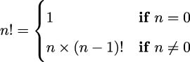
The preceding formula can be implemented in Python by using the following function definition:
def fact(n: int) -> int:
    if n == 0:
        return 1
    else:
        return n*fact(n-1)
This implementation has the advantage of simplicity. The recursion limits in Python artificially constrain us; we can’t do anything larger than about fact(997). The value of 1000! has 2,568 digits and generally exceeds our floating-point capacity; on some systems the floating-point limit is near 10300. Pragmatically, it’s common to switch to a log gamma function instead of working with immense numbers.
See https://functions.wolfram.com/GammaBetaErf/LogGamma/introductions/Gammas/ShowAll.html for more on log gamma functions.
We can expand Python’s call stack limit to stretch this to the limits of memory. It’s better, however, to manually optimize these kinds of functions to eliminate the recursion.
This function demonstrates a typical tail recursion. The last expression in the function is a call to the function with a new argument value. An optimizing compiler can replace the function call stack management with a loop that executes very quickly.
In this example, the function involves an incremental change from n to n − 1. This means that we’re generating a sequence of numbers and then doing a reduction to compute their product.
Stepping outside purely functional processing, we can define an imperative facti() calculation as follows:
def facti(n: int) -> int:
    if n == 0:
        return 1
    f = 1
    for i in range(2, n+1):
        f = f * i
    return f
This version of the factorial function will compute values beyond 1000! (2000!, for example, has 5,736 digits). This example isn’t purely functional. We’ve optimized the tail recursion into a stateful for statement depending on the i variable to maintain the state of the computation.
In general, we’re obliged to do this in Python because Python can’t automatically do the tail-call optimization. There are situations, however, where this kind of optimization isn’t actually helpful. We’ll look at a few of them.
6.1.2 Leaving recursion in place
In some cases, the recursive definition is actually optimal. Some recursions involve a divide and conquer strategy that minimizes the work. One example of this is the algorithm for doing exponentiation by squaring. This works for computing values that have a positive integer exponent, like 264. We can state it formally as follows:

We’ve broken the process into three cases, easily written in Python as a recursion. Look at the following function definition:
def fastexp(a: float, n: int) -> float:
    if n == 0:
        return 1
    elif n % 2 == 1:
        return a * fastexp(a, n - 1)
    else:
        t = fastexp(a, n // 2)
        return t * t
For odd numbers, the fastexp() method is defined recursively. The exponent n is reduced by 1. A simple tail-recursion optimization would work for this case. It would not work for the even case, however.
For even numbers, the fastexp() recursion uses n // 2, chopping the problem into half of its original size. Since the problem size is reduced by a factor of 2, this case results in a significant speed-up of the processing.
We can’t trivially reframe this kind of function into a tail-call optimization loop. Since it’s already optimal, we don’t really need to optimize it further. The recursion limit in Python would impose the constraint of n ≤ 21000, a generous upper bound.
6.1.3 Handling difficult tail-call optimization
We can look at the definition of Fibonacci numbers recursively. The following is one widely used definition for the nth Fibonacci number, Fn:

A given Fibonacci number, Fn, is defined as the sum of the previous two numbers, Fn−1 + Fn−2. This is an example of multiple recursion: it can’t be trivially optimized as a simple tail recursion. However, if we don’t optimize it to a tail recursion, we’ll find it to be too slow to be useful.
The following is a naïve implementation:
def fib(n: int) -> int:
    if n == 0: return 0
    if n == 1: return 1
    return fib(n-1) + fib(n-2)
This suffers from a terrible multiple recursion problem. When computing the fib(n) value, we must compute the fib(n-1) and fib(n-2) values. The computation of the fib(n-1) value involves a duplicate calculation of the fib(n-2) value. The two recursive uses of the fib() function will more than duplicate the amount of computation being done.
Because of the left-to-right Python evaluation rules, we can evaluate values up to about fib(1000). However, we have to be patient. Very patient. (Trying to find the actual upper bound with the default stack size means waiting a long time before the RecursionError is raised.)
The following is one alternative, which restates the entire algorithm to use stateful variables instead of a simple recursion:
def fibi(n: int) -> int:
    if n == 0: return 0
    if n == 1: return 1
    f_n2, f_n1 = 1, 1
    for _ in range(2, n):
        f_n2, f_n1 = f_n1, f_n2 + f_n1
    return f_n1
Our stateful version of this function counts up from 0, unlike the recursion, which counts down from the initial value of n. This version is considerably faster than the recursive version.
What’s important here is that we couldn’t trivially optimize the fib() function recursion with an obvious rewrite. In order to replace the recursion with an imperative version, we had to look closely at the algorithm to determine how many stateful intermediate variables were required.
As an exercise for the reader, try using the @cache decorator from the functools module. What impact does this have?
6.1.4 Processing collections through recursion
When working with a collection, we can also define the processing recursively. We can, for example, define the map() function recursively. The formalism could be stated as follows:
![( |{ [] if len(C ) = 0 map (f,C ) = | ( map(f,C [:−1]) + [f (C −1)] if len(C ) > 0](https://imgdetail.ebookreading.net/2023/10/9781803232577/9781803232577__9781803232577__files__Images__file52.jpg)
We’ve defined the mapping of a function, f, to an empty collection as an empty sequence, []. We’ve also specified that applying a function to a collection can be defined recursively with a three-step expression. First, recursively perform the mapping of the function to all of the collection except the last element, creating a sequence object. Then apply the function to the last element. Finally, append the last calculation to the previously built sequence.
Following is a purely recursive function version of this map() function:
from collections.abc import Callable, Sequence
from typing import Any, TypeVar

MapD = TypeVar("MapD")
MapR = TypeVar("MapR")

def mapr(
        f: Callable[[MapD], MapR],
        collection: Sequence[MapD]
) -> list[MapR]:
    if len(collection) == 0: return []
    return mapr(f, collection[:-1]) + [f(collection[-1])]
The value of the mapr(f,[]) method is defined to be an empty list object. The value of the mapr() function with a non-empty list will apply the function to the last element in the list and append this to the list built recursively from the mapr() function applied to the head of the list.
We have to emphasize that this mapr() function actually creates a list object. The built-in map() function is an iterator; it doesn’t create a list object. It yields the result values as they are computed. Also, the work is done in right-to-left order, which is not the way Python normally works. This is only observable when using a function that has side effects, something we’d like to avoid doing.
While this is an elegant formalism, it still lacks the tail-call optimization required. An optimization will allow us to exceed the default recursion limit of 1,000 and also performs much more quickly than this naïve recursion.
The use of Callable[[Any], Any] is a weak type hint. To be more clear, it can help to define a domain type variable and a range type variable. We’ll include this detail in the optimized example.
6.1.5 Tail-call optimization for collections
We have two general ways to handle collections: we can use a higher-order function that returns a generator expression, or we can create a function that uses a for statement to process each item in a collection. These two patterns are very similar.
Following is a higher-order function that behaves like the built-in map() function:
from collections.abc import Callable, Iterable, Iterator
from typing import Any, TypeVar

DomT = TypeVar("DomT")
RngT = TypeVar("RngT")

def mapf(
        f: Callable[[DomT], RngT],
        C: Iterable[DomT]
) -> Iterator[RngT]:
    return (f(x) for x in C)
We’ve returned a generator expression that produces the required mapping. This uses the explicit for in the generator expression as a kind of tail-call optimization.
The source of data, C, has a type hint of Iterable[DomT] to emphasize that some type, DomT, will form the domain for the mapping. The transformation function has a hint of Callable[[DomT], RngT] to make it clear that it transforms from some domain type to a range type. The function float(), for example, can transform values from the string domain to the float range. The result has the hint of Iterator[RngT] to show that it iterates over the range type, RngT; the result type of the callable function.
The following is a generator function with the same signature and result:
def mapg(
        f: Callable[[DomT], RngT],
        C: Iterable[DomT]
) -> Iterator[RngT]:
    for x in C:
        yield f(x)
This uses a complete for statement for the tail-call optimization. The results are identical. This version is slightly slower because it involves multiple statements.
In both cases, the result is an iterator over the results. We must do something else to materialize a sequence object from an iterable source. For example, here is the list() function being used to create a sequence from the iterator:
>>> list(mapg(lambda x: 2 ** x, [0, 1, 2, 3, 4]))
[1, 2, 4, 8, 16]
For performance and scalability, this kind of tail-call optimization is required in Python programs. It makes the code less than purely functional. However, the benefit far outweighs the lack of purity. In order to reap the benefits of succinct and expressive functional design, it is helpful to treat these less-than-pure functions as if they were proper recursions.
What this means, pragmatically, is that we must avoid cluttering up a collection processing function with additional stateful processing. The central tenets of functional programming are still valid even if some elements of our programs are less than purely functional.
6.1.6 Using the assignment (sometimes called the ”walrus”) operator in recursions
In some cases, recursions involve conditional processing that can be optimized using the ”walrus” or assignment operator, :=. The use of assignment means that we’re introducing stateful variables. If we’re careful of the scope of those variables, the possibility of terribly complex algorithms is reduced.
We reviewed the fast_exp() function shown below in the Leaving recursion in place section. This function used three separate cases to implement a divide and conquer strategy. In the case of raising a number, a, to an even power, we can use t = a![]() to compute t × t = an:
to compute t × t = an:
def fastexp_w(a: float, n: int) -> float:
    if n == 0:
        return 1
    else:
        q, r = divmod(n, 2)
        if r == 1:
            return a * fastexp_w(a, n - 1)
        else:
            return (t := fastexp_w(a, q)) * t
This uses the := walrus operator to compute a partial answer, fastexp_w(a, q), and save it into a temporary variable, t. This is used later in the same statement to compute t * t.
For the most part, when we perform tail-call optimization on a recursion, the body of the for statement will have ordinary assignment statements. It isn’t often necessary to exploit the walrus operator.
The assignment operator is often used in situations like regular expression matching, where we want to save the match object as well as make a decision. It’s very common to see if (match := pattern.match(text)): as a way to both attempt a regular expression match, save the resulting match object, and confirm it’s not a None object.
6.2 Reductions and folding a collection from many items to one
We can consider the sum() function to have the following kind of definition. We could say that the sum of a collection is 0 for an empty collection. For a non-empty collection, the sum is the first element plus the sum of the remaining elements:
![(| { 0 if n = 0 sum ([c0,c1,c2,...,cn]) = | ( c0 + sum ([c1,c2,...,cn]) if n > 0](https://imgdetail.ebookreading.net/2023/10/9781803232577/9781803232577__9781803232577__files__Images__file54.jpg)
We can use a slightly simplified notation called the Bird-Meertens Formalism. This uses ⊕∕[c0,c1,...cn] to show how some arbitrary binary operator, ⊕, can be applied to a sequence of values. It’s used as follows to summarize a recursive definition into something a little easier to work with:
We’ve effectively folded the + operator between each item of the sequence. Implicitly, the processing will be done left to right. This could be called a ”fold left” way of reducing a collection to a single value. We could also imagine grouping the operators from right to left, calling this a ”fold right.” While some compiled languages will perform this optimization, Python works strictly from left to right when given a sequence of similar precedence operators.
In Python, a product function can be defined recursively as follows:
from collections.abc import Sequence

def prodrc(collection: Sequence[float]) -> float:
    if len(collection) == 0: return 1
    return collection[0] * prodrc(collection[1:])
This is a tiny rewrite from a mathematical notation to Python. However, it is less than optimal because all of the slices will create a large number of intermediate list objects. It’s also limited to only working with explicit collections; it can’t work easily with iterable objects.
We can revise this slightly to work with an iterable, which avoids creating any intermediate collection objects. The following is a properly recursive product function that works with any iterator as a source of data:
from collections.abc import Iterator

def prodri(items: Iterator[float]) -> float:
    try:
        head = next(items)
    except StopIteration:
        return 1
    return head * prodri(items)
This doesn’t work with iterable collections. We can’t interrogate an iterator with the len() function to see how many elements it has. All we can do is attempt to extract the head of the iterator. If there are no items in the iterator, then any attempt to get the head will raise the StopIteration exception. If there is an item, then we can multiply this item by the product of the remaining items in the sequence.
Note that we must explicitly create an iterator from a materialized sequence object, using the iter() function. In other contexts, we might have an iterable result that we can use. Following is an example:
>>> prodri(iter([1,2,3,4,5,6,7]))
5040
This recursive definition does not rely on explicit state or other imperative features of Python. While it’s more purely functional, it is still limited to working with collections of under 1,000 items. (While we can extend the stack size, it’s far better to optimize this properly.) Pragmatically, we can use the following kind of imperative structure for reduction functions:
from collections.abc import Iterable

def prodi(items: Iterable[float]) -> float:
    p: float = 1
    for n in items:
        p *= n
    return p
This avoids any recursion limits. It includes the required tail-call optimization. Furthermore, this will work equally well with any iterable. This means a Sequence object, or an iterator.
6.2.1 Tail-call optimization using deques
The heart of recursion is a stack of function calls. Evaluating fact(5), for example, is 5*fact(4). The value of fact(4) is 5*fact(3). There is a stack of pending computations until fact(0) has a value of 1. Then the stack of computations is completed, revealing the final result.
Python manages the stack of calls for us. It imposes an arbitrary default limit of 1,000 calls on the stack, to prevent a program with a bug in the recursion from running forever.
We can manage the stack manually, also. This gives us another way to optimize recursions. We can—explicitly—create a stack of pending work. We can then do a final summarization of the pending work, emptying the items from the stack.
For something as simple as computing a factorial value, the stacking and unstacking can seem like needless overhead. For more complex applications, like examining the hierarchical file system, it seems more appropriate to mix processing files with putting directories onto a stack for later consideration.
We need a function to traverse a directory hierarchy without an explicit recursion. The core concept is that a directory is a collection of entries, and each entry is either a file, a sub-directory, or some other filesystem object we don’t want to touch (e.g., a mount point, symbolic link, etc.).
We can say a node in the directory tree is a collection of entries: N = e0,e1,e2,...,en. Each entry is either another directory, e ∈?, or a file, e ∈?.
We can perform mappings on each file in the tree to process each file’s content. We might perform a filter operation to create an iterator over files with a specific property. We can also perform a reduction to count the number of files with a property. In this example, we’ll count the occurrences of a specific substring throughout the contents of files in a directory tree.
Formally, we want a function p(f) that will provide the count of "print" in a node of the directory tree. It could be defined like this:
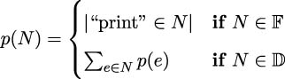
This shows how to apply the p(N) function to each element of a directory tree. When the element is a file, e ∈?, we can count instances of ”print”. When the element is a directory, e ∈?, we need to apply the p(N) function recursively to each entry, ex, in the directory. While directory trees can’t be deep enough to break Python’s stack size limit, this kind of algorithm reveals an alternative tail-call optimization. It is an opportunity to use an explicit stack.
The collections.deque class is a marvelous way to build stacks and queues. The name comes from ”double-ended queue,” sometimes spelled dequeue. The data structure can be used as either a last-in-first-out (LIFO) stack or a first-in-first-out (FIFO). In this example, we use the append() and pop() methods, which enforce LIFO stack behavior. While this is much like a list, there are some optimizations in the deque implementation that can make it slightly faster than the generic list.
Using a stack data structure lets us work with a hierarchy of indefinite size without running into Python’s internal stack depth limitation and raising RecursionError exceptions. The following function will traverse a file hierarchy looking at Python source files (with a suffix of .py):
from collections import deque
from pathlib import Path

def all_print(start: Path) -> int:
    count = 0
    pending: deque[Path] = deque([start])
    while pending:
        dir_path = pending.pop()
        for path in dir_path.iterdir():
            if path.is_file():
                if path.suffix == ’.py’:
                    count += path.read_text().count("print")
            elif path.is_dir():
                if not path.stem.startswith(’.’):
                    pending.append(path)
            else:  # Ignore other filesystem objects
                pass
    return count
We seeded the stack of pending tasks with the initial directory. The essential algorithm is to unstack a directory and visit each entry in the directory. For entries that are files with the proper suffix, the processing is performed: counting the occurrences of ”print”. For entries that are directories, the directory is put into the stack as a pending task. Note that directories with a leading dot in their name need to be ignored. For the code in this book, those directories include caches used by tools like mypy, pytest, and tox. We want to skip over those cache directories.
The processing performed on each file is part of the all_print() function. This can be refactored as a separate function that’s applied to each node as part of a reduction. Rewriting the all_print() function to be a proper higher-order function is left as an exercise for the reader.
The idea here is we have two strategies for transforming a formal recursion into a usefully optimized function. We can reframe the recursion into an iteration, or we can introduce an explicit stack.
In the next section, we will apply the idea of a reduction (and the associated tail-call optimizations) to creating groups of items and computing a reduction for the groups.
6.3 Group-by reduction from many items to fewer
The idea of a reduction can apply in many ways. We’ve looked at the essential recursive definition of a reduction that produces a single value from a collection of values. This leads us to optimizing the recursion so we have the ability to compute summaries without the overheads of a naive Pythonic implementation.
Creating subgroups in Python isn’t difficult, but it can help to understand the formalisms that support it. This understanding can help to avoid implementations that perform extremely poorly.
A very common operation is a reduction that groups values by some key or indicator. The raw data is grouped by some column’s value, and reductions (sometimes called aggregate functions) are applied to other columns.
In SQL, this is often called the GROUP BY clause of the SELECT statement. The SQL aggregate functions include SUM, COUNT, MAX, and MIN, and often many more.
Python offers us several ways to group data before computing a reduction of the grouped values. We’ll start by looking at two ways to get simple counts of grouped data. Then we’ll look at ways to compute different summaries of grouped data.
We’ll use the trip data that we computed in Chapter 4, Working with Collections. This data started as a sequence of latitude-longitude waypoints. We restructured it to create legs represented by three-tuples of start, end, and distance for each leg. The data looks as follows:
(((37.5490162, -76.330295), (37.840832, -76.273834), 17.7246),
((37.840832, -76.273834), (38.331501, -76.459503), 30.7382),
((38.331501, -76.459503), (38.845501, -76.537331), 31.0756),
...
((38.330166, -76.458504), (38.976334, -76.473503), 38.8019))
We’d like to know the most common distance. Since the data is real-valued, and continuous, each distance is a unique value. We need to constrain these values from the continuous domain to a discrete set of distances. For example, quantizing each leg to the nearest multiple of five nautical miles. This creates bands of 0 to 5 miles, over 5 to 10 miles, etc. Once we’ve created discrete integer values, we can count the number of legs in each of these bands.
These quantized distances can be produced with a generator expression:
quantized = (5 * (dist // 5) for start, stop, dist in trip)This will divide each distance by 5—discarding any fractions—then multiply the truncated result by 5 to compute a number that represents the distance rounded down to the nearest 5 nautical miles.
We don’t use the values assigned to the start and stop variables. It’s common practice to assign these values to the _ variable. This can lead to some confusion because this can obscure the structure of the triple. It would look like this:
quantized = (5 * (dist // 5) for _, _, dist in trip)This approach can be helpful for removing some visual clutter.
6.3.1 Building a mapping with Counter
A mapping like the collections.Counter class is a great optimization for doing reductions that create counts (or totals) grouped by some value in the collection. The following expression creates a mapping from distance to frequency:
# See Chapter 4 for ways to parse "file:./Winter%202012-2013.kml"
# We want to build a trip variable with the sequence of tuples

>>> from collections import Counter

>>> quantized = (5 * (dist // 5) for start, stop, dist in trip)
>>> summary = Counter(quantized)
The resulting summary object is stateful; it can be updated. The expression to create the groups, Counter(), looks like a function, making it a good fit for a design based on functional programming ideas.
If we print the summary.most_common() value, we’ll see the following results:
>>> summary.most_common()
[(30.0, 15), (15.0, 9), ...]
The most common distance was about 30 nautical miles. We can also apply functions like min() and max() to find the shortest recorded and longest legs as well.
Note that your output may vary slightly from what’s shown. The results of the most_common() function are in order of frequency; equal-frequency bins may be in any order. These five lengths may not always be in the order shown:
(35.0, 5), (5.0, 5), (10.0, 5), (20.0, 5), (25.0, 5)This slight variability makes testing with the doctest tool a little bit more complex. One helpful trick for testing with counters is to use a dictionary to validate the results in general; the comparison between actual and expected no longer relies on the vagaries of internal hash computations.
6.3.2 Building a mapping by sorting
An alternative to Counter is to sort the original collection, and then use a recursive loop to identify when each group begins. This involves materializing the raw data, performing a sort that could—at worst—do O(nlog n) operations, and then doing a reduction to get the sums or counts for each key.
In order to work in a general way with Python objects that can be sorted, we need to define the protocol required for sorting. We’ll call the protocol SupportsRichComparisonT because we can sort any kinds of objects that implement the rich comparison operators, < and >. This isn’t a particular class of objects; it’s a protocol that any number of classes might implement. We formalize the idea of a protocol that classes must support using the typing.Protocol type definition. It could be also be called an interface that a class must implement. Python’s flexibility stems from having a fairly large number of protocols that many different classes support.
The following is a common algorithm for creating groups from sorted data:
from collections.abc import Iterable
from typing import Any, TypeVar, Protocol, TypeAlias

class Comparable(Protocol):
    def __lt__(self, __other: Any) -> bool: ...
    def __gt__(self, __other: Any) -> bool: ...
SupportsRichComparisonT = TypeVar("SupportsRichComparisonT", bound=Comparable)

Leg: TypeAlias = tuple[Any, Any, float]

def group_sort(trip: Iterable[Leg]) -> dict[int, int]:

    def group(
            data: Iterable[SupportsRichComparisonT]
    ) -> Iterable[tuple[SupportsRichComparisonT, int]]:
        sorted_data = iter(sorted(data))
        previous, count = next(sorted_data), 1
        for d in sorted_data:
            if d == previous:
                count += 1
            else:
                yield previous, count
                previous, count = d, 1
        yield previous, count

    quantized = (int(5 * (dist // 5)) for beg, end, dist in trip)
    return dict(group(quantized))
The internal group() function steps through the sorted sequence of legs. If a given item key has already been seen—it matches the value in previous—then the counter variable is incremented. If a given item does not match the previous value, then there’s been a change in value: emit the previous value and the count, and begin a new accumulation of counts for the new value.
The definition of group() provides two important type hints. The source data is an iterable over some type, shown with the type variable SupportsRichComparisonT. In this specific case, it’s pretty clear that the values in use will be of type int; however, the algorithm will work for any Python type. The resulting iterable from the group() function will preserve the type of the source data, and this is made explicit by using the same type variable, SupportsRichComparisonT.
The final line of the group_sort() function creates a dictionary from the grouped items. This dictionary will be similar to a Counter dictionary. The primary difference is that a Counter() function will have a most_common() method function, which a default dictionary lacks.
We can also do this with itertools.groupby(). We’ll look at this function closely in Chapter 8, The Itertools Module.
6.3.3 Grouping or partitioning data by key values
There are no limits to the kinds of reductions we might want to apply to grouped data. We might have data with a number of independent and dependent variables. We can consider partitioning the data by an independent variable and computing summaries such as the maximum, minimum, average, and standard deviation of the values in each partition.
The essential trick to doing more sophisticated reductions is to collect all of the data values into each group. The Counter() function merely collects counts of identical items. For deeper analysis, we want to create sequences of the original members of the group.
Looking back at our trip data, each five-mile bin could contain the entire collection of legs of that distance, not merely a count of the legs. We can consider the partitioning as a recursion or as a stateful application of defaultdict(list) objects. We’ll look at the recursive definition of a groupby() function, since it’s easy to design.
Clearly, the groupby(C, key) computation for an empty collection, [], is the empty dictionary, dict(). Or, more usefully, the empty defaultdict(list) object.
For a non-empty collection, we need to work with item C[0], the head, and recursively process sequence C[1:], the tail. We can use slice expressions, or we can use the head, *tail = C statement to do this parsing of the collection, as follows:
>>> C = [1,2,3,4,5]
>>> head, *tail = C
>>> head
1
>>> tail
[2, 3, 4, 5]
If we have a defaultdict object named groups, we need to use the expression groups[key(head)].append(head) to include the head element in the groups dictionary. After this, we need to evaluate the groupby(tail, key) expression to process the remaining elements.
We can create a function as follows:
from collections import defaultdict
from collections.abc import Callable, Sequence, Hashable
from typing import TypeVar

SeqItemT = TypeVar("SeqItemT")
ItemKeyT = TypeVar("ItemKeyT", bound=Hashable)

def group_by(
        key: Callable[[SeqItemT], ItemKeyT],
        data: Sequence[SeqItemT]
) -> dict[ItemKeyT, list[SeqItemT]]:

    def group_into(
            key: Callable[[SeqItemT], ItemKeyT],
            collection: Sequence[SeqItemT],
            group_dict: dict[ItemKeyT, list[SeqItemT]]
    ) -> dict[ItemKeyT, list[SeqItemT]]:
        if len(collection) == 0:
            return group_dict
        head, *tail = collection
        group_dict[key(head)].append(head)
        return group_into(key, tail, group_dict)

    return group_into(key, data, defaultdict(list))
The interior function group_into() handles the essential recursive definition. An empty value for collection returns the provided dictionary, group_dict. A non-empty collection is partitioned into a head and tail. The head is used to update the group_dict dictionary. The tail is then used, recursively, to update the dictionary with all remaining elements.
The type hints make an explicit distinction between the type of the source objects SeqItemT and the type of the key ItemKeyT. The function provided as the key parameter must be a callable that returns a value of the key type ItemKeyT, given an object of the source type SeqItemT. In many of the examples, a function to extract the distance from a Leg object will be be shown. This is a Callable[[SeqItemT], ItemKeyT] where the source type SeqItemT is the Leg object and the key type ItemKeyT is the float value.
bound=Hashable is an additional constraint. This defines an ”upper bound” on the possible types, alerting mypy that any type that could be assigned to this type variable must implement the protocol for Hashable. The essential, immutable Python types of numbers, strings, and tuples all meet this bound. A mutable object like a dictionary, set, or list, will not meet the upper bound, leading to warnings from mypy.
We can’t easily use Python’s default values to collapse this into a single function. We explicitly cannot use the following incorrect command snippet:
# Bad use of a mutable default value

def group_by(key, data, dictionary=defaultdict(list)):
If we try this, all uses of the group_by() function share one common defaultdict(list) object. This does not work because Python builds the default value just once. Mutable objects as default values rarely do what we want. The common practice is to provide a None value, and use an explicit if statement to create each unique, empty instance of defaultdict(list) as needed. We’ve shown how to use a wrapper function definition to avoid the if statement.
We can group the data by distance as follows:
>>> binned_distance = lambda leg: 5 * (leg[2] // 5)
>>> by_distance = group_by(binned_distance, trip)
We’ve defined a reusable lambda that puts our distances into bins, each of which is 5 nautical miles in size. We then grouped the data using the provided lambda.
We can examine the binned data as follows:
>>> import pprint
>>> for distance in sorted(by_distance):
...     print(distance)
...     pprint.pprint(by_distance[distance])
The following is what the output looks like:
0.0
[((35.505665, -76.653664), (35.508335, -76.654999), 0.1731),
 ((35.028175, -76.682495), (35.031334, -76.682663), 0.1898),
 ((25.4095, -77.910164), (25.425833, -77.832664), 4.3155),
 ((25.0765, -77.308167), (25.080334, -77.334), 1.4235)]
5.0
[((38.845501, -76.537331), (38.992832, -76.451332), 9.7151),
 ((34.972332, -76.585167), (35.028175, -76.682495), 5.8441),
 ((30.717167, -81.552498), (30.766333, -81.471832), 5.103),
 ((25.471333, -78.408165), (25.504833, -78.232834), 9.7128),
 ((23.9555, -76.31633), (24.099667, -76.401833), 9.844)]
...
125.0
[((27.154167, -80.195663), (29.195168, -81.002998), 129.7748)]
Having looked at a recursive definition, we can turn to looking at making a tail-call optimization to build a group-by algorithm using iteration. This will work with larger collections of data, because it can exceed the internal stack size limitation.
We’ll start with doing tail-call optimization on the group_into() function. We’ll rename this to partition() because partitioning is another way of looking at grouping.
The partition() function can be written as an iteration as follows:
from collections import defaultdict
from collections.abc import Callable, Hashable, Iterable
from typing import TypeVar

SeqT = TypeVar("SeqT")
KeyT = TypeVar("KeyT", bound=Hashable)

def partition(
        key: Callable[[SeqT], KeyT],
        data: Iterable[SeqT]
) -> dict[KeyT, list[SeqT]]:
    group_dict = defaultdict(list)
    for head in data:
        group_dict[key(head)].append(head)
        #---------------------------------
    return group_dict
When doing the tail-call optimization, the essential line of the code in the imperative version will match the recursive definition. We’ve put a comment under the changed line to emphasize the rewrite is intended to have the same outcome. The rest of the structure represents the tail-call optimization we’ve adopted as a common way to work around the Python limitations.
The type hints emphasize the distinction between the source type SeqT and the key type KeyT. The source data can be anything, but the keys are limited to types that have proper hash values.
6.3.4 Writing more general group-by reductions
Once we have partitioned the raw data, we can compute various kinds of reductions on the data elements in each partition. We might, for example, want the northernmost point for the start of each leg in the distance bins.
We’ll introduce some helper functions to decompose the tuple as follows:
# Legs are (start, end, distance) tuples

start = lambda s, e, d: s

end = lambda s, e, d: e

dist = lambda s, e, d: d

# start and end of a Leg are (lat, lon) tuples

latitude = lambda lat, lon: lat

longitude = lambda lat, lon: lon
Each of these helper functions expects a tuple object to be provided using the * operator to map each element of the tuple to a separate parameter of the lambda. Once the tuple is expanded into the s, e, and p parameters, it’s reasonably obvious to return the proper parameter by name. It’s much clearer than trying to interpret the tuple_arg[2] value.
The following is how we use these helper functions:
>>> point = ((35.505665, -76.653664), (35.508335, -76.654999), 0.1731)
>>> start(*point)
(35.505665, -76.653664)

>>> end(*point)
(35.508335, -76.654999)

>>> dist(*point)
0.1731

>>> latitude(*start(*point))
35.505665
Our initial point object is a nested three tuple with (0)—a starting position, (1)—the ending position, and (2)—the distance. We extracted various fields using our helper functions.
Given these helpers, we can locate the northernmost starting position for the legs in each bin:
>>> binned_distance = lambda leg: 5 * (leg[2] // 5)
>>> by_distance = partition(binned_distance, trip)
>>> for distance in sorted(by_distance):
...     print(
...         distance,
...         max(by_distance[distance],
...         key=lambda pt: latitude(*start(*pt)))
...     )
The data that we grouped by distance included each leg of the given distance. We supplied all of the legs in each bin to the max() function. The key function we provided to the max() function extracted just the latitude of the starting point of the leg.
This gives us a short list of the northernmost legs of each distance, as follows:
0.0 ((35.505665, -76.653664), (35.508335, -76.654999), 0.1731)
5.0 ((38.845501, -76.537331), (38.992832, -76.451332), 9.7151)
10.0 ((36.444168, -76.3265), (36.297501, -76.217834), 10.2537)
...
125.0 ((27.154167, -80.195663), (29.195168, -81.002998), 129.7748)
6.3.5 Writing higher-order reductions
We’ll look at an example of a higher-order reduction algorithm here. This will introduce a rather complex topic. The simplest kind of reduction develops a single value from a collection of values. Python has a number of built-in reductions, including any(), all(), max(), min(), sum(), and len().
As we noted in Chapter 4, Working with Collections, we can do a great deal of statistical calculation if we start with a few reductions such as the following:
from collections.abc import Sequence

def sum_x0(data: Sequence[float]) -> float:
    return sum(1 for x in data)  # or len(data)

def sum_x1(data: Sequence[float]) -> float:
    return sum(x for x in data)  # or sum(data)

def sum_x2(data: Sequence[float]) -> float:
    return sum(x*x for x in data)
This allows us to define mean, standard deviation, normalized values, correction, and even least-squares linear regression, building on these base reduction functions.
The last of our reductions, sum_x2(), shows how we can apply existing reductions to create higher-order functions. We might change our approach to be more like the following:
from collections.abc import Callable, Iterable
from typing import Any

def sum_f(
        function: Callable[[Any], float],
        data: Iterable[float]
) -> float:
    return sum(function(x) for x in data)
We’ve added a function, function(), as a parameter; the function can transform the data. This overall function, sum_f(), computes the sum of the transformed values.
Now we can apply this function in three different ways to compute the three essential sums as follows:
>>> data = [7.46, 6.77, 12.74, 7.11, 7.81,
...     8.84, 6.08, 5.39, 8.15, 6.42, 5.73]

>>> N = sum_f(lambda x: 1, data)  # x**0
>>> N
11
>>> S = sum_f(lambda x: x, data)  # x**1
>>> round(S, 2)
82.5
>>> S2 = sum_f(lambda x: x*x, data)  # x**2
>>> round(S2, 4)
659.9762
We’ve plugged in a small lambda to compute ∑ x∈Xx0 = ∑ x∈X1, which is the count, ∑ x∈Xx1 = ∑ x∈Xx, the sum, and ∑ x∈Xx2, the sum of the squares, which we can use to compute standard deviation.
A common extension to this includes a filter to reject raw data that is unknown or unsuitable in some way. We might use the following function to reject bad data:
from collections.abc import Callable, Iterable

def sum_filter_f(
        filter_f: Callable[[float], bool],
        function: Callable[[float], float],
        data: Iterable[float]
) -> float:
    return sum(function(x) for x in data if filter_f(x))
The following function definition for computing a mean will reject None values in a simple way:
valid = lambda x: x is not None

def mean_f(predicate: Callable[[Any], bool], data: Sequence[float]) -> float:
    count_ = lambda x: 1
    sum_ = lambda x: x
    N = sum_filter_f(valid, count_, data)
    S = sum_filter_f(valid, sum_, data)
    return S / N
This shows how we can provide two distinct combinations of lambdas to our sum_filter_f() function. The filter argument is a lambda that rejects None values; we’ve called it valid to emphasize its meaning. The function argument is a lambda that implements a count or a sum operation. We can easily add a lambda to compute a sum of squares.
The reuse of a common valid rule assures that the various computations are all identical in applying any filters to the source data. This can be combined with a user-selected filter criteria to provide a tidy plug-in to compute a number of statistics related to a user’s requested subset of the data.
6.3.6 Writing file parsers
We can often consider a file parser to be a kind of reduction. Many languages have two levels of definition: the lower-level tokens in the language and the higher-level structures built from those tokens. When looking at an XML file, the tags, tag names, and attribute names form this lower-level syntax; the structures which are described by XML form a higher-level syntax.
The lower-level lexical scanning is a kind of reduction that takes individual characters and groups them into tokens. This fits well with Python’s generator function design pattern. We can often write functions that look as follows:
from collections.abc import Iterator
from enum import Enum
import re

class Token(Enum):
    SPACE = 1
    PARA = 2
    EOF = 3

def lexical_scan(some_source: str) -> Iterator[tuple[Token, str]]:
    previous_end = 0
    separator_pat = re.compile(r"
s*
", re.M|re.S)
    for sep in separator_pat.finditer(some_source):
        start, end = sep.span()
        yield Token.PARA, some_source[previous_end: start]
        yield Token.SPACE, some_source[start: end]
        previous_end = end
    yield Token.PARA, some_source[previous_end:]
    yield Token.EOF, ""
For well-known file formats, we’ll use existing file parsers. For data in CSV, JSON, XML, or TOML format, we don’t need to write file parsers. Most of these modules have a load() method that produces useful Python objects.
In some cases, we’ll need to combine the results of this parsing into higher-level objects, useful for our specific application. While the CSV parser provides individual rows, these might need to be used to create NamedTuple instances, or perhaps some other class of immutable Python objects. Our examples of trip data, starting in Chapter 4, Working with Collections, are combined into higher-level objects, legs of a journey, by an algorithm that combines waypoints into pairs. When we introduce more complex decision-making, we make a transition from restructuring into parsing.
In order to provide useful waypoints in the first place, we needed to parse a source file. In these examples, the input was a KML file; KML is an XML representation of geographic information. The essential features of the parser look similar to the following definition:
from collections.abc import Iterator
from typing import TextIO, cast

def comma_split(text: str) -> list[str]:
    return text.split(",")

def row_iter_kml(file_obj: TextIO) -> Iterator[list[str]]:
    ns_map = {
        "ns0": "http://www.opengis.net/kml/2.2",
        "ns1": "http://www.google.com/kml/ext/2.2"}
    xpath = (
        "./ns0:Document/ns0:Folder/"
        "ns0:Placemark/ns0:Point/ns0:coordinates")
    doc = XML.parse(file_obj)
    return (
        comma_split(cast(str, coordinates.text))
        for coordinates in doc.findall(xpath, ns_map)
    )
The bulk of the row_iter_kml() function is the XML parsing that allows us to use the doc.findall() function to iterate through the <ns0:coordinates> tags in the document. We’ve used a function named comma_split() to parse the text of this tag into a three-tuple of values.
The cast() function is only present to provide evidence to mypy that the value of coordinates.text is a str object. The default definition of the text attribute is Union[str, bytes]; in this application, the data will be str exclusively. The cast() function doesn’t do any runtime processing.
This function focused on working with the normalized XML structure. The document is close to the database designer’s definitions of first normal form: each attribute is atomic (a single value), and each row in the XML data has the same columns with data of a consistent type. The data values aren’t fully atomic, however: we have to split the points on the , to separate longitude, latitude, and altitude into atomic string values. However, the text value for these XML tags is internally consistent, making it a close fit with first normal form.
A large volume of data—XML tags, attributes, and other punctuation—is reduced to a somewhat smaller volume, including just floating-point latitude and longitude values. For this reason, we can think of parsers as a kind of reduction.
We’ll need a higher-level set of conversions to map the tuples of text into floating-point numbers. Also, we’d like to discard altitude, and reorder longitude and latitude. This will produce the application-specific tuple we need. We can use functions as follows for this conversion:
from collections.abc import Iterator

def pick_lat_lon(
        lon: str, lat: str, alt: str
) -> tuple[str, str]:
    return lat, lon

def float_lat_lon(
        row_iter: Iterator[list[str]]
) -> Iterator[tuple[float, float]]:
    lat_lon_iter = (
        pick_lat_lon(*row)
        for row in row_iter
    )
    return (
        (float(lat), float(lon))
        for lat, lon in lat_lon_iter
    )
The essential tool is the float_lat_lon() function. This is a higher-order function that returns a generator expression. The generator uses the map() function to apply the float() function conversion to the results of the pick_lat_lon() function, and the *row argument to assign each member of the row tuple to a different parameter of the pick_lat_lon() function. This only works when each row is a three-tuple. The pick_lat_lon() function then returns a two-tuple of the selected items in the required order.
The source includes XML that looks like this:
<Placemark><Point>
<coordinates>-76.33029518659048, 37.54901619777347,0</coordinates>
</Point></Placemark>
We can use this parser as follows:
>>> import urllib.request
>>> source_url = "file:./Winter%202012-2013.kml"
>>> with urllib.request.urlopen(source_url) as source:
...      flat = list(float_lat_lon(row_iter_kml(source)))
This will build a tuple-of-tuples representation of each waypoint along the path in the original KML file. The result will be a flat sequence of pairs that looks like this:
>>> from pprint import pprint
>>> pprint(flat)  # doctest: +ELLIPSIS
[(37.54901619777347, -76.33029518659048),
 ...
 (38.976334, -76.473503)]
The float_lat_lon() function uses a low-level XML parser to extract rows of text data from the original representation. It uses a higher-level parser to transform the text items into more useful tuples of floating-point values suitable for the target application.
Parsing CSV files
In Chapter 3, Functions, Iterators, and Generators, we saw another example where we parsed a CSV file that was not in a normalized form: we had to discard header rows to make it useful. To do this, we used a function that extracted the header and returned an iterator over the remaining rows.
The data looks as follows:
Anscombe’s quartet
I II III IV
x y x y x y x y
10.0 8.04 10.0 9.14 10.0 7.46 8.0 6.58
8.0 6.95 8.0 8.14 8.0 6.77 8.0 5.76
...
5.0 5.68 5.0 4.74 5.0 5.73 8.0 6.89
The columns are separated by tab characters. Plus, there are three rows of headers that we can discard.
Here’s another version of that CSV-based parser. We’ve broken it into three functions. The first, row_iter_csv() function, returns the iterator over the rows in a tab-delimited file. The function looks as follows:
from collections.abc import Iterator
import csv
from typing import TextIO

def row_iter_csv(source: TextIO) -> Iterator[list[str]]:
    rdr = csv.reader(source, delimiter="	")
    return rdr
This is a small wrapper around the CSV parsing process. When we look back at the previous parsers for XML and plain text, this was the kind of thing that was missing from those parsers. Producing an iterable over row tuples can be a common feature of parsers for normalized data.
Once we have a row of tuples, we can pass rows that contain usable data and reject rows that contain other metadata, such as titles and column names. We’ll introduce a helper function that we can use to do some of the parsing, plus a filter() function to validate a row of data.
Following is the conversion:
from typing import cast

def float_none(data: str) -> float | None:
    try:
        data_f = float(data)
        return data_f
    except ValueError:
        return None
This function handles the conversion of a single string to float values, converting bad data to a None value. The type hint of float | None expresses the idea of having a value of the given type or having a value of the same type as None. This can also be stated as Union[float, None] to show how the result is a union of different alternative types.
We can embed the float_none() function in a mapping so that we convert all columns of a row to a float or None value. A lambda for this looks as follows:
from collections.abc import Callable
from typing import TypeAlias

R_Float: TypeAlias = list[float | None]

float_row: Callable[[list[str]], R_Float] =
    lambda row: list(map(float_none, row))
Two type hints are used to make the definition of the float_row() function explicit. The R_Float hint defines the floating-point version of a row of data that may include None values.
Following is a row-level validator based on the use of the all() function to ensure that all values are float (or none of the values are None):
all_numeric: Callable[[R_Float], bool] =
    lambda row: all(row) and len(row) == 8
This lambda is a kind of reduction, transforming a row of floating-point values to a Boolean value if all values are not ”falsy” (that is, neither None nor zero) and there are exactly eight values.
The simplistic all_numeric() function conflates zero and None. A more sophisticated test would rely on something such as not any(item is None for item in row). The rewrite is left as an exercise for the reader.
The essential design is to create row-based elements that can be combined to create more complete algorithms for parsing an input file. The foundational functions iterate over tuples of text. These are combined to convert and validate the converted data. For the cases where files are either in first normal form (all rows are the same) or a simple validator can reject the extraneous rows, this design pattern works out nicely.
All parsing problems aren’t quite this simple, however. Some files have important data in header or trailer rows that must be preserved, even though it doesn’t match the format of the rest of the file. These non-normalized files will require a more sophisticated parser design.
Parsing plain text files with headers
In Chapter 3, Functions, Iterators, and Generators, the Crayola.GPL file was presented without showing the parser. This file looks as follows:
GIMP Palette
Name: Crayola
Columns: 16
#
239 222 205 Almond
205 149 117 Antique Brass
We can parse a text file using regular expressions. We need to use a filter to read (and parse) header rows. We also want to return an iterable sequence of data rows. This rather complex two-part parsing is based entirely on the two-part—head and tail—file structure.
Following is a low-level parser that handles both the four lines of the header and the long tail:
from collections.abc import Iterator
from typing import TextIO, TypeAlias

Head_Body: TypeAlias = tuple[tuple[str, str], Iterator[list[str]]]

def row_iter_gpl(file_obj: TextIO) -> Head_Body:
    header_pat = re.compile(
        r"GIMP Palette
Name:s*(.*?)
Columns:s*(.*?)
#
",
        re.M)

    def read_head(file_obj: TextIO) -> tuple[tuple[str, str], TextIO]:
        if match := header_pat.match(
            "".join(file_obj.readline() for _ in range(4))
        ):
            return (match.group(1), match.group(2)), file_obj
        else:
            raise ValueError("invalid header")

    def read_tail(
            headers: tuple[str, str],
            file_obj: TextIO) -> Head_Body:
        return (
            headers,
            (next_line.split() for next_line in file_obj)
        )

    return read_tail(*read_head(file_obj))
The Head_Body type definition summarizes the overall goal of the row iterator. The result is a two-tuple. The first item is a two-tuple with details from the file header. The second item is an iterator that provides the text items for a color definition. This Head_Body type hint is used in two places in this function definition.
The header_pat regular expression parses all four lines of the header. There are instances of () in the expression to extract the name and column information from the header.
There are two internal functions for parsing different parts of the file. The read_head() function parses the header lines and returns interesting text and a TextIO object that can be used for the rest of the parsing. It does this by reading four lines and merging them into a single long string. This is then parsed with the header_pat regular expression.
The idea of returning the iterator from one function to be used in another function is a pattern for passing an explicitly stateful object from one function to another. It seems helpful to make sure all of the arguments for the read_tail() function are the results from the read_head() function.
The read_tail() function parses the iterator over the remaining lines. These lines are merely split on spaces, since that fits the description of the GPL file format.
For more information, visit the following link: https://code.google.com/p/grafx2/issues/detail?id=518.
Once we’ve transformed each line of the file into a canonical tuple-of-strings format, we can apply the higher level of parsing to this data. This involves conversion and (if necessary) validation.
The following is a higher-level parser command snippet:
from collections.abc import Iterator
from typing import NamedTuple

class Color(NamedTuple):
    red: int
    blue: int
    green: int
    name: str

def color_palette(
        headers: tuple[str, str],
        row_iter: Iterator[list[str]]
) -> tuple[str, str, tuple[Color, ...]]:
    name, columns = headers
    colors = tuple(
        Color(int(r), int(g), int(b), " ".join(name))
        for r, g, b, *name in row_iter
    )
    return name, columns, colors
This function will work with the output of the lower-level row_iter_gpl() parser: it requires the headers and the iterator over individual rows. This function will use the multiple assignment feature of the for clause in the generator to separate the color numbers and the remaining words into four variables, r, g, b, and name. The use of the *name parameter ensures that all remaining values will be assigned to the name variable as a tuple. The " ".join(name) expression then concatenates the words into a single space-separated string.
The following is how we can use this two-tier parser:
>>> from pathlib import Path
>>> source_path = Path("crayola.gpl")
>>> with source_path.open() as source:
...     name, cols, colors = color_palette(
...         *row_iter_gpl(source)
...     )
>>> name
’Crayola’
>>> cols
’16’
>>> len(colors)
133
We’ve applied the higher-level parser to the results of the lower-level parser. This will return the headers and a tuple built from the sequence of Color objects.
6.4 Summary
In this chapter, we’ve looked at two significant functional programming topics. We’ve looked at recursions in some detail. Many functional programming language compilers will optimize a recursive function to transform a call in the tail of the function to a loop. This is sometimes called tail recursion elimination. More commonly, it’s known as tail-call optimization. In Python, we must do the tail-call optimization manually by using an explicit for statement, replacing a purely functional recursion.
We’ve also looked at reduction algorithms, including sum(), count(), max(), and min() functions. We looked at the collections.Counter() function and related groupby() reductions.
We’ve also looked at how parsing (and lexical scanning) are similar to reductions since they transform sequences of tokens (or sequences of characters) into higher-order collections with more complex properties. We’ve examined a design pattern that decomposes parsing into a lower level and tries to produce tuples of raw strings, and a higher level that creates more useful application objects.
In the next chapter, we’ll look at some techniques appropriate to working with named tuples and other immutable data structures. We’ll look at techniques that make stateful objects unnecessary. While stateful objects aren’t purely functional, the idea of a class hierarchy can be used to package related method definitions.
6.5 Exercises
This chapter’s exercises are based on code available from Packt Publishing on GitHub. See https://github.com/PacktPublishing/Functional-Python-Programming-3rd-Edition.
In some cases, the reader will notice that the code provided on GitHub includes partial solutions to some of the exercises. These serve as hints, allowing the reader to explore alternative solutions.
In many cases, exercises will need unit test cases to confirm they actually solve the problem. These are often identical to the unit test cases already provided in the GitHub repository. The reader should replace the book’s example function name with their own solution to confirm that it works.
6.5.1 Multiple recursion and caching
In Handling difficult tail-call optimization, we looked at a naive definition of a function to compute Fibonacci numbers, the fib() function. The functools.cache decorator can have a profound impact on the performance of this algorithm.
Implement both versions and describe the impact of caching on the time required to compute large Fibonacci numbers.
6.5.2 Refactor the all_print() function
In Tail-call optimization using deques, we showed a function that used a collections.deque to visit all nodes in a directory tree, summing the value for each node that is a proper file. This can be done with a list as well as a deque, with some minor code changes.
This function embedded a specific computation. This computation (finding all occurrences of ”print”) really should have been a separate function. The body of the all_print() function should be refactored into two functions:
A generic directory traverse that applies a function to each text file with the expected suffix and sums the results.
A function that counts instances of ”print” in a given Python file.
6.5.3 Parsing CSV files
See the Parsing CSV files section, earlier in this chapter. In that example, the simplistic all_numeric() function conflates zero and None.
Create a test case for this function that will show that it does not handle zero correctly, treating it as None. Once the test case is defined, rewrite the all_numeric() function to distinguish between zero and None.
Note that it’s common practice in Python to use the is operator when comparing with None. This specifically avoids some subtle problems that can arise when a class has an implementation of __eq__() that doesn’t handle None as a properly distinct object.
6.5.4 Classification of state, Part III
See Chapter 5, Higher-Order Functions, the Classification of state exercise.
There’s a third way to consume status details and summarize them.
Write a reduce computation. This starts with an initial state of Running. As each service’s three-tuple is folded into the result, there is a comparison between the state and the three-tuple. If the three-tuple has a non-responsive service, the state advances to Stopped. If the three-tuple has a slow or not working service, the state advances to Degraded. If no problems are found, the initial value becomes the final health of the overall system.
The idea is to provide a status_add(previous, this_service) function. This can be used in the context of status = reduce(status_add, service_status_sequence, "Running") to compute the current status of the sequence of services.
6.5.5 Diesel engine data
A diesel engine has had some repairs that raised doubts about the accuracy of the tachometer. After some heroic effort, the following table of data was collected showing the observed reading on the engine’s tachometer, and the actual RPMs measured with an optical device on the engine.
| Sample | Tach | Engine |
| 1 | 1000 | 883 |
| 2 | 1500 | 1242 |
| 3 | 1500 | 1217 |
| 4 | 1600 | 1306 |
| 5 | 1750 | 1534 |
| 6 | 2000 | 1805 |
| 7 | 2000 | 1720 |
If needed, create a CSV file with the data. If you have access to the GitHub repository for this book, this is available in the engine.csv file.
Create a NamedTuple for each sample and write some functions to acquire this data in a useful form. Once the data is available, see the Using sums and counts for statistics section of Chapter 4, Working with Collections, for a definition of a correlation function.
The objective is to apply this correlation function to the engine and tach values to see if the values correlate. If they do, it suggests that the engine’s instruments can be recalibrated. If they don’t correlate, something else is wrong with the engine.
Note that the Chapter 4, Working with Collections, correlation example may have assumptions about data types that don’t necessarily apply to the NamedTuple defined earlier. If necessary, rewrite the type hints or your NamedTuple definition. Note that it can be difficult to write perfectly generic type hints, and it often takes a bit of work to resolve the differences.
Join our community Discord space
Join our Python Discord workspace to discuss and know more about the book: https://packt.link/dHrHU
