2.1 Functions as first-class objects

Functional programming is often succinct and expressive. One way to achieve this is by providing functions as arguments and return values for other functions. We’ll look at numerous examples of manipulating functions.

For this to work, functions must be first-class objects in the runtime environment. In programming languages such as C, a function is not a runtime object; because the compiled C code generally lacks internal attributes and methods, there’s little runtime introspection that can be performed on a function. In Python, however, functions are objects that are created (usually) by def statements and can be manipulated by other Python functions. We can also create a function as a callable object or by assigning a lambda object to a variable.

Here’s how a function definition creates an object with attributes:

>>> def example(a, b, **kw): 
...     return a*b 
... 
>>> type(example) 
<class ’function’> 
>>> example.__code__.co_varnames 
(’a’, ’b’, ’kw’) 
>>> example.__code__.co_argcount 
2

We’ve created an object, example, that is of the function class. This object has numerous attributes. The __code__ attribute of the function object has attributes of its own. The implementation details aren’t important. What is important is functions are first-class objects and can be manipulated like all other objects. The example shows the values of two of the many attributes of a function object.

>>> mersenne = lambda x: 2 ** x - 1 
>>> mersenne(17) 
131071

>>> default_zip = lambda row: row.setdefault(’ZIP’, ’00000’)

>>> r_0 = {’CITY’: ’Vaca Key’} 
>>> default_zip(r_0) 
’00000’ 
>>> r_0 
{’CITY’: ’Vaca Key’, ’ZIP’: ’00000’} 
 
>>> r_1 = {’CITY’: ’Asheville’, ’ZIP’: 27891} 
>>> default_zip(r_1) 
27891

>>> year_cheese = [(2000, 29.87), (2001, 30.12), 
...     (2002, 30.6), (2003, 30.66), (2004, 31.33), 
...     (2005, 32.62), (2006, 32.73), (2007, 33.5), 
...     (2008, 32.84), (2009, 33.02), (2010, 32.92)]

>>> max(year_cheese) 
(2010, 32.92)

>>> max(year_cheese, key=lambda yc: yc[1]) 
(2007, 33.5)

2.2 Immutable data

Since we’re not using variables to track the state of a computation, our focus needs to stay on immutable objects. We can make extensive use of tuples, typing.NamedTuples, and frozen @dataclass to provide more complex data structures that are also immutable. We’ll look at these class definitions in detail in Chapter 7, Complex Stateless Objects.

The idea of immutable objects is not foreign to Python. Strings and tuples are two widely-used immutable objects. There can be a performance advantage to using immutable tuples instead of more complex mutable objects. In some cases, the benefits come from rethinking the algorithm to avoid the costs of object mutation.

As an example, here’s a common design pattern that works well with immutable objects: the wrapper() function. A list of tuples is a fairly common data structure. We will often process this list of tuples in one of the two following ways:

• Using higher-order functions: As shown earlier, we provided a lambda as an argument to the max() function: max(year_cheese, key=lambda yc: yc[1]).

• Using the wrap-process-unwrap pattern: In a functional context, we can implement this with code that follows an unwrap(process(wrap(structure))) pattern.

For example, look at the following command snippet:

>>> max(map(lambda yc: (yc[1], yc), year_cheese))[1] 
(2007, 33.5)

This fits the three-part pattern of wrapping a data structure, finding the maximum of the wrapped structures, and then unwrapping the structure.

The expression map(lambda yc: (yc[1], yc), year_cheese) will transform each item into a two-tuple with a key followed by the original item. In this example, the comparison key value is the expression yc[1].

The processing is done using the max() function. Since each piece of the source data has been simplified to a new two-tuple, the higher-order function features of the max() function aren’t required. To make this work, the comparison value was taken from position one of the source record and placed first into the two-tuple. The default behavior of the max() function uses the first item in each two-tuple to locate the largest value.

Finally, we unwrap using the subscript expression [1]. This will pick the second element of the two-tuple selected by the max() function.

This kind of wrap-and-unwrap is so common that some languages have special functions with names like fst() and snd() that we can use as function prefixes instead of a syntactic suffix of [0] or [1]. We can use this idea to modify our wrap-process-unwrap example, as follows:

>>> snd = lambda x: x[1] 
>>> snd(max(map(lambda yc: (yc[1], yc), year_cheese))) 
(2007, 33.5)

Here, a lambda is used to define the snd() function to pick the second item from a tuple. This provides an easier-to-read version of unwrap(process(wrap())). As with the previous example, the map(lambda... , year_cheese) expression is used to wrap our raw data items, and the max() function does the processing. Finally, the snd() function extracts the second item from the tuple.

This can be simplified by using typing.NamedTuple or a @dataclass. In Chapter 7, Complex Stateless Objects, we’ll look at these two alternatives.

We will—as a general design principle—avoid class definitions. It can seem like anathema to avoid objects in an Object-Oriented Programming (OOP) language, but we note that functional programming doesn’t depend on stateful objects. When we use class definitions, we’ll avoid designs that update attribute values.

There are a number of good reasons for using immutable objects. We can, for example, use an object as a named collection of attribute values. Additionally, callable objects can provide some optimizations, like the caching of computed results. Caching is important because Python doesn’t have an optimizing compiler. Another reason for using class definitions is to provide a namespace for closely related functions.

2.3 Strict and non-strict evaluation

Functional programming’s efficiency stems, in part, from being able to defer a computation until it’s required. There are two similar concepts for avoiding computation. These are:

• Strictness: Python operators are generally strict and evaluate all sub-expressions from left to right. This means an expression like f(a)+f(b)+f(c) is evaluated as if it was (f(a)+f(b))+f(c). An optimizing compiler might avoid strict ordering to improve performance. Python doesn’t optimize and code is mostly strict. We’ll look at cases where Python is not strict below.

• Eagerness and laziness: Python operators are generally eager and evaluate all sub-expressions to compute the final answer. This means (3-3) * f(d) is fully evaluated even though the first part of the multiplication—the (3-3) sub-expression—is always zero, meaning the result is always zero, no matter what value is computed by the expression f(d). Generator expressions are an example of Python doing lazy evaluation. We’ll look at an example of this in the next section, Lazy and eager evaluation.

In Python, the logical expression operators and, or, and if-else are all non-strict. We sometimes call them short-circuit operators because they don’t need to evaluate all arguments to determine the resulting value.

The following command snippet shows the and operator’s non-strict feature:

>>> 0 and print("right") 
0 
 
>>> True and print("right") 
right

When we execute the first of the preceding command snippets, the left-hand side of the and operator is equivalent to False; the right-hand side is not evaluated. In the second example, when the left-hand side is equivalent to True, the right-hand side is evaluated.

Other parts of Python are strict. Outside the logical operators, an expression is evaluated strictly from left to right. A sequence of statement lines is also evaluated strictly in order. Literal lists and tuples require strict evaluation. When a class is created, the methods are defined in a strict order.

2.4 Lazy and eager evaluation

Python’s generator expressions and generator functions are lazy. These expressions don’t create all possible results immediately. It’s difficult to see this without explicitly logging the details of a calculation. Here is an example of the version of the range() function that has the side effect of showing the numbers it creates:

from collections.abc import Iterator 
def numbers(stop: int) -> Iterator[int]: 
    for i in range(stop): 
        print(f"{i=}") 
        yield i

To provide some debugging hints, this function prints each value as the value is yielded. If this function were eager, evaluating numbers(1024) would take the time (and storage) to create all 1,024 numbers. Since the numbers() function is lazy, it only creates a number as it is requested.

We can use this noisy numbers() function in a way that will show lazy evaluation. We’ll write a function that evaluates some, but not all, of the values from this iterator:

def sum_to(limit: int) -> int: 
    sum: int = 0 
    for i in numbers(1_024): 
        if i == limit: break 
        sum += i 
    return sum

The sum_to() function has type hints to show that it should accept an integer value for the n parameter and return an integer result. This function will not evaluate the entire result of the values produced by the numbers() function. It will break after only consuming a few values from the numbers() function. We can see this consumption of values in the following log:

>>> sum_to(5) 
i=0 
i=1 
i=2 
i=3 
i=4 
i=5 
10

As we’ll see later, Python generator functions have some properties that make them a little awkward for simple functional programming. Specifically, a generator can only be used once in Python. We have to be cautious with how we use the lazy Python generator expressions.

2.5 Recursion instead of an explicit loop state

Functional programs don’t rely on loops and the associated overhead of tracking the state of loops. Instead, functional programs try to rely on the much simpler approach of recursive functions. In some languages, the programs are written as recursions, but Tail-Call Optimization (TCO) in the compiler changes them to loops. We’ll introduce some recursion here and examine it closely in Chapter 6, Recursions and Reductions.

We’ll look at an iteration to test whether a number is a prime number. Here’s a definition from https://mathworld.wolfram.com/PrimeNumber.html: “A prime number ... is a positive integer p > 1 that has no positive integer divisors other than 1 and p itself.” We can create a naive and poorly performing algorithm to determine whether a number has any factors between 2 and the number. This is called the Trial Division algorithm. It has the advantage of simplicity; it works acceptably for solving some of the Project Euler problems. Read up on Miller-Rabin primality tests for a much better algorithm.

We’ll use the term coprime to mean that two numbers have only 1 as their common factor. The numbers 2 and 3, for example, are coprime. The numbers 6 and 9, however, are not coprime because they have 3 as a common factor.

If we want to know whether a number, n, is prime, we actually ask this: is the number n coprime to all prime numbers, p, such that p² < n? We can simplify this using all integers, i, such that 2 ≤ i² < n. The simplification does more work, but is much easier to implement.

Sometimes, it helps to formalize this as follows:

The expression could look as follows in Python:

not any( 
    n % p == 0 
    for p in range(2, int(math.sqrt(n))+1) 
)

An alternative conversion from mathematical formalism to Python would use all(n % p != 0, ...). The all() function will stop when it finds the first False value. The not any() will stop when it finds the first True value. While the results are identical, the performance varies depending on whether or not p is a prime number.

This expression has a for iteration inside it: it’s not a pure example of stateless functional programming. We can reframe this into a function that works with a collection of values. We can ask whether the number, n, is coprime within any value in the half-open interval [2, + 1). This uses the symbols [) to show a half-open interval: the lower values are included, and the upper value is not included. This is typical behavior of the Python range() function. We will also restrict ourselves to the domain of natural numbers. The square root values, for example, are implicitly truncated to integers.

We can think of the definition of prime as the following:

given n > 1. We know n is prime when it is coprime to all values in the range [2, + 1).

While the formal math can feel daunting, this is a search for a coprime in the given range of values. If we find a coprime, the value of n is not prime. If we fail to find a coprime, then the value of n must be prime.

When defining a recursive search over a range of values, the base case can be the empty range. Searching the empty range means no values can be found. Searching a non-empty range is handled recursively by processing one value combined with a range that’s narrower by the one value processed. We could formalize it as follows:

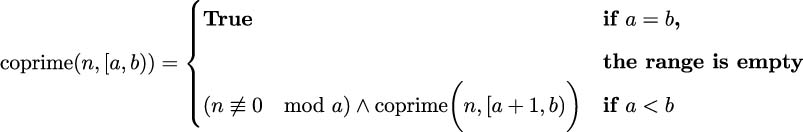
In the case where the range is non-empty, one value, a, is checked to see if it is coprime with n; then, the remaining values in the range [a + 1,b) are checked. This expression can be confirmed by providing concrete examples of the two cases, which are given as follows:

• If the range is empty, a = b, we evaluated something like this:

  

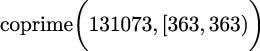
  The range contains no values, so the return is True. This is analogous to computing the sum of an empty list: the sum is zero.

• If the range is not empty, we evaluated something like this:

  

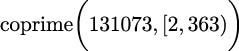
  This decomposes into evaluating:

  

  For this example, we can see that the first clause is True, and we’ll evaluate the second clause recursively. Compare this with evaluating coprime16,. The value of 16≢0 mod 2 would be False; the values of 16 and 2 are not coprime. The evaluation of coprime131073, becomes irrelevant, since we know the 16 is composite.

As an exercise for the reader, this recursion can be redefined to count down instead of up, using [a,b− 1) in the second case. Try this revision to see what, if any, changes are required.

Here is a Python code snippet that implements this definition of prime:

def isprimer(n: int) -> bool: 
    def iscoprime(k: int, a: int, b: int) -> bool: 
        """Is k coprime with a value in the given range?""" 
        if a == b: return True 
        return (k % a != 0) and iscoprime(k, a+1, b) 
    return iscoprime(n, 2, int(math.sqrt(n)) + 1)

This shows a recursive definition of an iscoprime() function. The function expects an int value for all three parameters. The type hints claim it will return a bool result.

The recursion base case is implemented as a == b. When this is true, the range of values from a to one less than b is empty. Because the recursive evaluation of iscoprime() is the tail end of the function, this is an example of tail recursion.

The iscoprime() function is embedded in the isprimer() function. The outer function serves to establish the boundary condition for the range of values that will be searched.

What’s important in this example is that the two cases of this recursive function follow the mathematical definition in a direct way. Making the range of values an explicit argument to the internal iscoprime() function allows us to call the function recursively with argument values that reflect a steadily shrinking interval.

While recursion is often succinct and expressive, we have to be cautious about using it in Python. There are two problems that can arise:

• Python imposes a recursion limit to detect recursive functions with improperly defined base cases.

• Python does not have a compiler that does Tail-Call Optimization (TCO) for us.

The default recursion limit is 1,000, which is adequate for many algorithms. It’s possible to change this with the sys.setrecursionlimit() function. It’s not wise to raise this arbitrarily since it might lead to exceeding the OS memory limitations and crashing the Python runtime.

If we try a recursive isprimer() function on a prime number n over 1,000,000, we’ll run afoul of the recursion limit. (Folks using IPython have a higher default limit on the size of the stack; try isprimer(9_000_011) to see the problem.)

Some functional programming languages can optimize these “tail call” recursive functions. An optimizing compiler will transform the recursive evaluation of the iscoprime(k, a+1, b) expression into a low-overhead for statement. The optimization tends to make debugging optimized programs more difficult. Python doesn’t perform this optimization. Performance and memory are sacrificed for clarity and simplicity. This also means we are forced to do the optimization manually.

This is the subject of Chapter 6, Recursions and Reductions. We’ll look at several examples of doing manual TCO.

2.6 Functional type systems

Some functional programming languages, such as Haskell and Scala, are statically compiled, and depend on declared types for functions and their arguments. To provide the kind of flexibility Python already has, these languages have sophisticated type-matching rules allowing a generic function to work for a variety of related types.

In object-oriented Python, we often use the class inheritance hierarchy instead of sophisticated function type matching. We rely on Python to dispatch an operator to a proper method based on simple name-matching rules.

Python’s built-in ”duck typing” rules offer a great deal of type flexibility. The more complex type matching rules for a compiled functional language aren’t relevant. It’s common to define a typing.Protocol to specify the features an object must have. The actual class hierarchy doesn’t matter; what matters is the presence of the appropriate methods and attributes.

Python’s match statement offers a number of structure and type matching capabilities. Because the match statement has so many alternatives, we’ll return to it several times. For now, we’ll provide an introductory example to show the core syntax.

Here’s an example that relies on literal matching, wildcard matching with _, and guard conditions:

import math 
def isprimem(n: int) -> bool: 
    match n: 
        case _ if n < 2: 
            prime = False 
        case 2: 
            prime = True 
        case _ if n % 2 == 0: 
            prime = False 
        case _: 
            for i in range(3, 1 + int(math.sqrt(n)), 2): 
                if n % i == 0: 
                    # Stop as soon as we know... 
                    return False 
            prime = True 
    return prime

When working with a single data type, the match statement is not dramatically simpler than an if-elif chain. The case _ blocks use the _ pattern, which matches anything without binding any variables. Some of these are followed by additional guards, for example, if n < 2, to provide a more nuanced decision to these cases.

The final case _: matches any possible value not matched by any of the prior case blocks. It is analogous to the else: clause in an if statement.

The single return statement at the end is expected by mypy. We could rewrite this to use return statements for each case. While it would work properly, without a single, clear return it’s difficult for the mypy tool to confirm that the match statement truly covers all possible conditions.

As we look at other examples, we’ll see more of the power of the pattern and type matching capabilities. This example matches literal values of a single type. The match statement can do quite a bit more. In later chapters, we’ll see the distinction between type hints, checked by a tool like mypy, and type matching that can be done by the match statement.

2.7 Familiar territory

One of the ideas that emerges from the previous list of topics is that many functional programming constructs are already present in Python. Indeed, elements of functional programming are already a very typical and common part of OOP.

As a very specific example, a fluent Application Program Interface (API) is a very clear example of functional programming. If we take time to create a class with return self in each method, we can use it as follows:

some_object.foo().bar().yet_more()

We can just as easily write several closely related functions that work as follows:

yet_more(bar(foo(some_object)))

We’ve switched the syntax from traditional object-oriented suffix notation to a more functional prefix notation. Python uses both notations freely, often using a prefix version of a special method name. For example, the len() function is generally implemented by the __len__() class special method.

Of course, the implementation of the preceding class might involve a highly stateful object. Even then, a small change in viewpoint may reveal a functional approach that can lead to more succinct or more expressive programming.

The point is not that imperative programming is broken in some way, or that functional programming offers a vastly superior technology. The point is that functional programming leads to a change in viewpoint that can, in many cases, be helpful for designing succinct, expressive programs.

2.8 Learning some advanced concepts

We will set some more advanced concepts aside for consideration in later chapters. These concepts are part of the implementation of a purely functional language. Since Python isn’t purely functional, our hybrid approach won’t require deep consideration of these topics.

We will identify these here for the benefit of readers who already know a functional language such as Haskell and are learning Python. The underlying concerns are present in all programming languages, but we’ll tackle them differently in Python. In many cases, we can and will drop into imperative programming rather than use a strictly functional approach.

The topics are as follows:

• Referential transparency: When looking at lazy evaluation and the various kinds of optimizations that are possible in a compiled language, the idea of multiple routes to the same object is important. In Python, this isn’t as important because there aren’t any relevant compile-time optimizations.

• Currying: The type systems will employ currying to reduce multiple-argument functions to single-argument functions. We’ll look at currying in some depth in Chapter 12, Decorator Design Techniques.

• Monads: These are purely functional constructs that allow us to structure a sequential pipeline of processing in a flexible way. In some cases, we’ll resort to imperative Python to achieve the same end. We’ll also leverage the elegant PyMonad library for this. We’ll defer this until Chapter 13, The PyMonad Library.

2.9 Summary

In this chapter, we’ve identified a number of features that characterize the functional programming paradigm. We started with first-class and higher-order functions. The idea is that a function can be an argument to a function or the result of a function. When functions become the object of additional programming, we can write some extremely flexible and generic algorithms.

The idea of immutable data is sometimes odd in an imperative and object-oriented programming language such as Python. When we start to focus on functional programming, however, we see a number of ways that state changes can be confusing or unhelpful. Using immutable objects can be a helpful simplification.

Python focuses on strict evaluation: all sub-expressions are evaluated from left to right through the statement. Python, however, does perform some non-strict evaluation. The or, and, and if-else logical operators are non-strict: all sub-expressions are not necessarily evaluated.

Generator functions can be described as lazy. While Python is generally eager, and evaluates all sub-expressions a soon as possible, we can leverage generator functions to create lazy evaluation. With lazy evaluation, a computation is not performed until it’s needed.

While functional programming relies on recursion instead of the explicit loop state, Python imposes some limitations here. Because of the stack limitation and the lack of an optimizing compiler, we’re forced to manually optimize recursive functions. We’ll return to this topic in Chapter 6, Recursions and Reductions.

Although many functional languages have sophisticated type systems, we’ll rely on Python’s dynamic type resolution. In some cases, this means we’ll have to write manual coercion for various types.

In the next chapter, we’ll look at the core concepts of pure functions and how these fit in with Python’s built-in data structures. Given this foundation, we can look at the higher-order functions available in Python and how we can define our own higher-order functions.

2.10 Exercises

This chapter’s exercises are based on code available from Packt Publishing on GitHub. See https://github.com/PacktPublishing/Functional-Python-Programming-3rd-Edition.

In some cases, the reader will notice that the code provided on GitHub includes partial solutions to some of the exercises. These serve as hints, allowing the reader to explore alternative solutions.

In many cases, exercises will need unit test cases to confirm they actually solve the problem. These are often identical to the unit test cases already provided in the GitHub repository. The reader should replace the book’s example function name with their own solution to confirm that it works.

2.10.1 Apply map() to a sequence of values

Some analysis has revealed a consistent measurement error in a device. The machine’s revolutions per minute (RPM) as displayed on the tachometer are consistently incorrect. (Gathering the true RPM involves some heroic engineering effort, but is not a sustainable way to manage the machine.)

The result is a model that translates observed, o, to actual, a:

The machine can only operate in the range of 800 to 2,500 RPM. Until the tachometer can be replaced with one that’s properly calibrated, we need a table of values from observed RPM to actual RPM. This can be printed and laminated and put near the machine to help gauge fuel consumption and workload.

Because the tachometer can only be read to the nearest 100 RPM, the table only needs to show values like 800, 900, 1000, 1100, ..., 2500.

The output should be something like the following:

Observed  Actual 
     800     630 
     900     720 
etc.

In order to provide a flexible solution, it helps to create the following two separate functions:

• A function to implement the model, which computes the actual value from the observation

• A function to display the table of values produced from the results of the model function

These two–separate–functions will be used as part of the recalibration effort for the piece of equipment.

Test cases for the model can be isolated from test cases for the table of values, allowing new models to be used as more data is gathered.

While it is the topic of a later chapter, and has only been mentioned here, use of map() is encouraged, but not required.