
5
Working with Genomes
Many tasks in computational biology are dependent on the existence of reference genomes. If you are performing sequence alignment, finding genes, or studying the genetics of populations, you will be directly or indirectly using a reference genome. In this chapter, we will develop some recipes for working with reference genomes and dealing with references of varying quality, which can range from high quality (by high quality, we only refer to the state of the genome’s assembly, which is the focus of this chapter), as with the human genome, to problematic with non-model species. We will also learn how to deal with genome annotations (working with databases that will point us to interesting features in the genome) and extract sequence data using the annotation information. We will also try to find some gene orthologs across species. Finally, we will access a Gene Ontology (GO) database.
In this chapter, we will cover the following recipes:
- Working with high-quality reference genomes
- Dealing with low-quality reference genomes
- Traversing genome annotations
- Extracting genes from a reference using annotations
- Finding orthologues with the Ensembl REST API
- Retrieving gene ontology information from Ensembl
Technical requirements
If you are running this chapter’s content via Docker, you can use the tiagoantao/bioinformatics_genomes image. If you are using Anaconda, the required software for this chapter will be introduced in each relevant section.
Working with high-quality reference genomes
In this recipe, you will learn about a few general techniques to manipulate reference genomes. As an illustrative example, we will study the GC content – the fraction of the genome that is based on guanine-cytosine in Plasmodium falciparum, the most important parasite species that causes malaria. Reference genomes are normally made available as FASTA files.
Getting ready
Organism genomes come in widely different sizes, ranging from viruses such as HIV, which is 9.7 kbp, to bacteria such as E. coli, to protozoans such as Plasmodium falciparum, which has a 22 Mbp spread across 14 chromosomes, mitochondrion, and apicoplast, to the fruit fly with three autosomes, a mitochondrion, and X/Y sex chromosomes, to humans with their three Gbp pairs spread across 22 autosomes, X/Y chromosomes, and mitochondria, all the way up to Paris japonica, a plant with 150 Gbp of the genome. Along the way, you have different ploidy and sex chromosome organizations.
Tip
As you can see, different organisms have very different genome sizes. This difference can be of several orders of magnitude. This can have significant implications for your programming style. Working with a large genome will require you to be more conservative with memory. Unfortunately, larger genomes would benefit from more speed-efficient programming techniques (as you have much more data to analyze); these are conflicting requirements. The general rule is that you have to be much more careful with efficiency (both speed and memory) with larger genomes.
To make this recipe less of a burden, we will use a small eukaryotic genome from Plasmodium falciparum. This genome still has many typical features of larger genomes (for example, multiple chromosomes). Therefore, it’s a good compromise between complexity and size. Note that with a genome that’s the size of Plasmodium falciparum, it will be possible to perform many operations by loading the whole genome in memory. However, we opted for a programming style that can be used with bigger genomes (for example, mammals) so that you can use this recipe in a more general way, but feel free to use more memory-intensive approaches with small genomes like this.
We will use Biopython, which you installed in Chapter 1, Python and the Surrounding Software Ecology. As usual, this recipe is available in this book’s Jupyter notebook as Chapter05/Reference_Genome.py, in the code bundle for this book. We will need to download the reference genome – you can find the up-to-date location in the aforementioned notebook. To generate the chart at the end of this recipe, we will need reportlab:
conda install -c bioconda reportlab
Now, we’re ready to begin.
How to do it...
Follow these steps:
- We will start by inspecting the description of all of the sequences in the reference genome’s FASTA file:
from Bio import SeqIO
genome_name = 'PlasmoDB-9.3_Pfalciparum3D7_Genome.fasta'
recs = SeqIO.parse(genome_name, 'fasta')
for rec in recs:
print(rec.description)
This code should look familiar from the previous chapter, Chapter 3, Next-Generation Sequencing. Let’s take a look at part of the output:

Figure 5.1 – The output showing the FASTA descriptions for the reference genome of Plasmodium falciparum
Different genome references will have different description lines, but they will generally contain important information. In this example, you can see that we have chromosomes, mitochondria, and apicoplast. We can also view the chromosome sizes, but we will take the value from the sequence length instead.
- Let’s parse the description line to extract the chromosome number. We will retrieve the chromosome size from the sequence and compute the GC content across chromosomes on a window basis:
from Bio import SeqUtils
recs = SeqIO.parse(genome_name, 'fasta')
chrom_sizes = {}
chrom_GC = {}
block_size = 50000
min_GC = 100.0
max_GC = 0.0
for rec in recs:
if rec.description.find('SO=chromosome') == -1:
continue
chrom = int(rec.description.split('_')[1])
chrom_GC[chrom] = []
size = len(rec.seq)
chrom_sizes[chrom] = size
num_blocks = size // block_size + 1
for block in range(num_blocks):
start = block_size * block
if block == num_blocks - 1:
end = size
else:
end = block_size + start + 1
block_seq = rec.seq[start:end]
block_GC = SeqUtils.GC(block_seq)
if block_GC < min_GC:
min_GC = block_GC
if block_GC > max_GC:
max_GC = block_GC
chrom_GC[chrom].append(block_GC)
print(min_GC, max_GC)
Here, we have performed a windowed analysis of all chromosomes, similar to what we did in Chapter 3, Next-Generation Sequencing. We started by defining a window size of 50 kbp. This is appropriate for Plasmodium falciparum (feel free to vary its size), but you will want to consider other values for genomes with chromosomes that are orders of magnitude different from this.
Note that we are re-reading the file. With such a small genome, it would have been feasible (in Step 1) to do an in-memory load of the whole genome. By all means, feel free to try this programming style for small genomes – it’s faster! However, our code is designed to be reused with larger genomes.
- Note that in the for loop, we ignore the mitochondrion and apicoplast by parsing the SO entry to the description. The chrom_sizes dictionary will maintain the size of chromosomes.
The chrom_GC dictionary is our most interesting data structure and will contain a list of a fraction of the GC content for each 50 kbp window. So, for chromosome 1, which has a size of 640,851 bp, there will be 14 entries because this chromosome’s size is 14 blocks of 50 kbp.
Be aware of two unusual features of the Plasmodium falciparum genome: the genome is very AT-rich – that is, GC-poor. Therefore, the numbers that you will get will be very low. Also, chromosomes are ordered based on size (as is common) but starting with the smallest size. The usual convention is to start with the largest size (such as with genomes in humans).
- Now, let’s create a genome plot of the GC distribution. We will use shades of blue for the GC content. However, for high outliers, we will use shades of red. For low outliers, we will use shades of yellow:
from reportlab.lib import colors
from reportlab.lib.units import cm
from Bio.Graphics import BasicChromosome
chroms = list(chrom_sizes.keys())
chroms.sort()
biggest_chrom = max(chrom_sizes.values())
my_genome = BasicChromosome.Organism(output_format="png")
my_genome.page_size = (29.7*cm, 21*cm)
telomere_length = 10
bottom_GC = 17.5
top_GC = 22.0
for chrom in chroms:
chrom_size = chrom_sizes[chrom]
chrom_representation = BasicChromosome.Chromosome ('Cr %d' % chrom)
chrom_representation.scale_num = biggest_chrom
tel = BasicChromosome.TelomereSegment()
tel.scale = telomere_length
chrom_representation.add(tel)
num_blocks = len(chrom_GC[chrom])
for block, gc in enumerate(chrom_GC[chrom]):
my_GC = chrom_GC[chrom][block]
body = BasicChromosome.ChromosomeSegment()
if my_GC > top_GC:
body.fill_color = colors.Color(1, 0, 0)
elif my_GC < bottom_GC:
body.fill_color = colors.Color(1, 1, 0)
else:
my_color = (my_GC - bottom_GC) / (top_GC -bottom_GC)
body.fill_color = colors.Color(my_color,my_color, 1)
if block < num_blocks - 1:
body.scale = block_size
else:
body.scale = chrom_size % block_size
chrom_representation.add(body)
tel = BasicChromosome.TelomereSegment(inverted=True)
tel.scale = telomere_length
chrom_representation.add(tel)
my_genome.add(chrom_representation)
my_genome.draw('falciparum.png', 'Plasmodium falciparum')
The first line converts the return of the keys method into a list. This was redundant in Python 2, but not in Python 3, where the keys method has a specific dict_keys return type.
We draw the chromosomes in order (hence the sort). We need the size of the biggest chromosome (14, in Plasmodium falciparum) to make sure that the size of chromosomes is printed with the correct scale (the biggest_chrom variable).
Then, we create an A4-sized representation of an organism with a PNG output. Note that we draw very small telomeres of 10 bp. This will produce a rectangular-like chromosome. You can make the telomeres bigger, giving them a roundish representation, or you may have the arguably better idea of using the correct telomere size for your species.
We declare that anything with a GC content below 17.5% or above 22.0% will be considered an outlier. Remember that for most other species, this will be much higher.
Then, we print these chromosomes: they are bounded by telomeres and composed of 50 kbp chromosome segments (the last segment is sized with the remainder). Each segment will be colored in blue, with a red-green component based on the linear normalization between two outlier values. Each chromosome segment will either be 50 kbp or potentially smaller if it’s the last one of the chromosome. The output is shown in the following diagram:

Figure 5.2 – The 14 chromosomes of Plasmodium falciparum, color-coded with the GC content (red is more than 22%, yellow less than 17%, and the blue shades represent a linear gradient between both numbers)
Tip
Biopython code evolved before Python was such a fashionable language. In the past, the availability of libraries was quite limited. The usage of reportlab can be seen mostly as a legacy issue. I suggest that you learn just enough from it to use it with Biopython. If you are planning on learning a modern plotting library in Python, then the standard bearer is Matplotlib, as we learned in Chapter 2, Getting to Know NumPy, pandas, Arrow, and Matplotlib. Alternatives include Bokeh, HoloViews, or Python’s version of ggplot (or even more sophisticated visualization alternatives, such as Mayavi, Visualization Toolkit (VTK), and even the Blender API).
- Finally, you can print the image inline in the notebook:
from IPython.core.display import Image
Image("falciparum.png")
And that completes this recipe!
There’s more...
Plasmodium falciparum is a reasonable example of a eukaryote with a small genome that allows you to perform a small data exercise with enough features, while still being useful for most eukaryotes. Of course, there are no sex chromosomes (such as X/Y in humans), but these should be easy to process because reference genomes do not deal with ploidy issues.
Plasmodium falciparum does have a mitochondrion, but we will not deal with it here due to space constraints. Biopython does have the functionality to print circular genomes, which you can also use with bacteria. With regards to bacteria and viruses, these genomes are much easier to process because their size is very small.
See also
Here are some sources you can learn more from:
- You can find many reference genomes of model organisms in Ensembl at http://www.ensembl.org/info/data/ftp/index.html.
- As usual, National Center for Biotechnology Information (NCBI) also provides a large list of genomes at http://www.ncbi.nlm.nih.gov/genome/browse/.
- There are plenty of websites dedicated to a single organism (or a set of related organisms). Apart from PlasmoDB (http://plasmodb.org/plasmo/), which you downloaded the Plasmodium falciparum genome from, you will find VectorBase (https://www.vectorbase.org/) in the next recipe for disease vectors. FlyBase (http://flybase.org/) for Drosophila melanogaster is also worth mentioning, but do not forget to search for your organism of interest.
Dealing with low-quality genome references
Unfortunately, not all reference genomes will have the quality of Plasmodium falciparum. Apart from some model species (for example, humans, or the common fruit fly Drosophila melanogaster) and a few others, most reference genomes could use some improvement. In this recipe, we will learn how to deal with reference genomes of lower quality.
Getting ready
In keeping with the malaria theme, we will use the reference genomes of two mosquitoes that are vectors of malaria: Anopheles gambiae (which is the most important vector of malaria and can be found in Sub-Saharan Africa) and Anopheles atroparvus, a malaria vector in Europe (while the disease has been eradicated in Europe, this vector is still around). The Anopheles gambiae genome is of reasonable quality. Most chromosomes have been mapped, although the Y chromosome still needs some work. There is a fairly large unknown chromosome, probably composed of bits of X and Y chromosomes, as well as midgut microbiota. This genome has a reasonable amount of positions that are not called (that is, you will find Ns instead of ACTGs). The Anopheles atroparvus genome is still in the scaffold format. Unfortunately, this is what you will find for many non-model species.
Note that we will up the ante a bit. The Anopheles genome is one order of magnitude bigger than the Plasmodium falciparum genome (but still one order of magnitude smaller than most mammals).
We will use Biopython, which you installed in Chapter 1, Python and the Surrounding Software Ecology. As usual, this recipe is available in this book’s Jupyter notebook at Chapter05/Low_Quality.py, in the code bundle for this book. At the start of the notebook, you can find the most up-to-date location of both genomes, along with the code to download them.
How to do it...
Follow these steps:
- Let’s start by listing the chromosomes of the Anopheles gambiae genome:
import gzip
from Bio import SeqIO
gambiae_name = 'gambiae.fa.gz'
atroparvus_name = 'atroparvus.fa.gz'
recs = SeqIO.parse(gzip.open(gambiae_name, 'rt', encoding='utf-8'), 'fasta')
for rec in recs:
print(rec.description)
This will produce an output that will include the organism chromosomes (along with a few unmapped supercontigs not depicted):
AgamP4_2L | organism=Anopheles_gambiae_PEST | version=AgamP4 | length=49364325 | SO=chromosome
AgamP4_2R | organism=Anopheles_gambiae_PEST | version=AgamP4 | length=61545105 | SO=chromosome
AgamP4_3L | organism=Anopheles_gambiae_PEST | version=AgamP4 | length=41963435 | SO=chromosome
AgamP4_3R | organism=Anopheles_gambiae_PEST | version=AgamP4 | length=53200684 | SO=chromosome
AgamP4_X | organism=Anopheles_gambiae_PEST | version=AgamP4 | length=24393108 | SO=chromosome
AgamP4_Y_unplaced | organism=Anopheles_gambiae_PEST | version=AgamP4 | length=237045 | SO=chromosome
AgamP4_Mt | organism=Anopheles_gambiae_PEST | version=AgamP4 | length=15363 | SO=mitochondrial_chromosome
The code is quite straightforward. We use the gzip module because the files of larger genomes are normally compressed. We can see four chromosome arms (2L, 2R, 3L, and 3R), the mitochondria (Mt), the X chromosome, and the Y chromosome, which is quite small and has a name that all but indicates that it may not be in the best state. Also, the unknown (UNKN) chromosome is a large proportion of the reference genome, to the tune of a chromosome arm.
Do not perform this with Anopheles atroparvus; otherwise, you will get more than a thousand entries, courtesy of the scaffold status.
- Now, let’s check the uncalled positions (Ns) and their distribution for the Anopheles gambiae genome:
recs = SeqIO.parse(gzip.open(gambiae_name, 'rt', encoding='utf-8'), 'fasta')
chrom_Ns = {}
chrom_sizes = {}
for rec in recs:
if rec.description.find('supercontig') > -1:
continue
print(rec.description, rec.id, rec)
chrom = rec.id.split('_')[1]
if chrom in ['UNKN']:
continue
chrom_Ns[chrom] = []
on_N = False
curr_size = 0
for pos, nuc in enumerate(rec.seq):
if nuc in ['N', 'n']:
curr_size += 1
on_N = True
else:
if on_N:
chrom_Ns[chrom].append(curr_size)
curr_size = 0
on_N = False
if on_N:
chrom_Ns[chrom].append(curr_size)
chrom_sizes[chrom] = len(rec.seq)
for chrom, Ns in chrom_Ns.items():
size = chrom_sizes[chrom]
if len(Ns) > 0:
max_Ns = max(Ns)
else:
max_Ns = 'NA'
print(f'{chrom} ({size}): %Ns ({round(100 * sum(Ns) / size, 1)}), num Ns: {len(Ns)}, max N: {max_Ns}')
The preceding code will take some time to run, so please be patient; we will inspect every base pair of autosomes. As usual, we will reopen and re-read the file to save memory.
We have two dictionaries: one dictionary that contains chromosome sizes and another that contains the distribution of the sizes of runs of Ns. To calculate the runs of Ns, we must traverse all autosomes (noting when an N position starts and ends). Then, we must print the basic statistics of the distribution of Ns:
2L (49364325): %Ns (1.7), num Ns: 957, max N: 28884
2R (61545105): %Ns (2.3), num Ns: 1658, max N: 36427
3L (41963435): %Ns (2.9), num Ns: 1272, max N: 31063
3R (53200684): %Ns (1.8), num Ns: 1128, max N: 24292
X (24393108): %Ns (4.1), num Ns: 1287, max N: 21132
Y (237045): %Ns (43.0), num Ns: 63, max N: 7957
Mt (15363): %Ns (0.0), num Ns: 0, max N: NA
So, for the 2L chromosome arm (with a size of 49 Mbp), 1.7% are N calls divided by 957 runs. The biggest run is 28884 bps. Note that the X chromosome has the highest fraction of positions with Ns.
- Now, let’s turn our attention to the Anopheles Atroparvus genome. Let’s count the number of scaffolds, along with the distribution of scaffold sizes:
import numpy as np
recs = SeqIO.parse(gzip.open(atroparvus_name, 'rt', encoding='utf-8'), 'fasta')
sizes = []
size_N = []
for rec in recs:
size = len(rec.seq)
sizes.append(size)
count_N = 0
for nuc in rec.seq:
if nuc in ['n', 'N']:
count_N += 1
size_N.append((size, count_N / size))
print(len(sizes), np.median(sizes), np.mean(sizes),
max(sizes), min(sizes),
np.percentile(sizes, 10), np.percentile(sizes, 90))
This code is similar to what we looked at previously, but we print slightly more detailed statistics using NumPy, so we get the following:
1320 7811.5 170678.2 58369459 1004 1537.1 39644.7
Thus, we have 1371 scaffolds (against seven entries on the Anopheles gambiae genome) with a median size of 7811.5 (a mean of 17,0678.2). The biggest scaffold is 5.8 Mbp, while the smallest scaffold is 1,004 bp. The tenth percentile for size is 1537.1, while the ninetieth is 39644.7.
- Finally, let’s plot the fraction of the scaffold – that is, N – as a function of its size:
import matplotlib.pyplot as plt
small_split = 4800
large_split = 540000
fig, axs = plt.subplots(1, 3, figsize=(16, 9), squeeze=False, sharey=True)
xs, ys = zip(*[(x, 100 * y) for x, y in size_N if x <= small_split])
axs[0, 0].plot(xs, ys, '.')
xs, ys = zip(*[(x, 100 * y) for x, y in size_N if x > small_split and x <= large_split])
axs[0, 1].plot(xs, ys, '.')
axs[0, 1].set_xlim(small_split, large_split)
xs, ys = zip(*[(x, 100 * y) for x, y in size_N if x > large_split])
axs[0, 2].plot(xs, ys, '.')
axs[0, 0].set_ylabel('Fraction of Ns', fontsize=12)
axs[0, 1].set_xlabel('Contig size', fontsize=12)
fig.suptitle('Fraction of Ns per contig size', fontsize=26)
The preceding code will generate the output shown in the following diagram, in which we split the chart into three parts based on the scaffold size: one for scaffolds with less than 4,800 bp, one for scaffolds between 4,800 and 540,000 bp, and one for larger ones. The fraction of Ns is very low for small scaffolds (always below 3.5%); for medium scaffolds, it has a large variance (sizes between 0% and above 90%), and a tighter variance (between 0% and 25%) for the largest scaffolds:

Figure 5.3 – The fraction of scaffolds that are N as a function of their size
There’s more...
Sometimes, reference genomes carry extra information. For example, the Anopheles gambiae genome is soft masked. This means that some procedures were run on the genome to identify areas of low complexity (which are normally more problematic to analyze). This can be annotated by capitalization: ACTG will be high complexity, whereas actg will be low.
Reference genomes with lots of scaffolds are more than an inconvenient hassle. For example, very small scaffolds (say, below 2,000 bp) may have mapping problems when using an aligner (such as Burrows-Wheeler Aligner (BWA)), especially at the extremes (most scaffolds will have mapping problems at their extremes, but these will be of a much larger proportion of the scaffold if it’s small). If you are using a reference genome like this to align, you will want to consider ignoring the pair information (assuming that you have paired-end reads) when mapping to small scaffolds, or at least measure the impact of the scaffold size on the performance of your aligner. In any case, the general idea is that you should be careful because the scaffold size and number will rear their ugly head from time to time.
With these genomes, only complete ambiguity (N) was identified. Note that other genome assemblies will give you an intermediate code between the total ambiguity and certainty (ACTG).
See also
Here are some resources you can learn more from:
- Tools such as RepeatMasker can be used to find areas of the genome with low complexity. Check out http://www.repeatmasker.org/ for more information.
- IUPAC ambiguity codes may be useful to have in hand when processing other genomes. Check out http://www.bioinformatics.org/sms/iupac.html for more information.
Traversing genome annotations
Having a genome sequence is interesting, but we will want to extract features from it, such as genes, exons, and coding sequences. This type of annotation information is made available in Generic Feature Format (GFF) and General Transfer Format (GTF) files. In this recipe, we will learn how to parse and analyze GFF files while using the annotation of the Anopheles gambiae genome as an example.
Getting ready
Use the Chapter05/Annotations.py notebook file, which is provided in the code bundle for this book. The up-to-date location of the GFF file that we will be using can be found at the top of the notebook.
You will need to install gffutils:
conda install -c bioconda gffutils
Now, we’re ready to start.
How to do it...
Follow these steps:
- Let’s start by creating an annotation database with gffutils, based on our GFF file:
import gffutils
import sqlite3
try:
    db = gffutils.create_db('gambiae.gff.gz', 'ag.db')
except sqlite3.OperationalError:
    db = gffutils.FeatureDB('ag.db')
The gffutils library creates a SQLite database to store annotations efficiently. Here, we will try to create the database, but if it already exists, we will use the existing one. This step can be time-consuming.
- Now, let’s list all the available feature types and count them:
print(list(db.featuretypes()))
for feat_type in db.featuretypes():
print(feat_type, db.count_features_of_type(feat_type))
These features will include contigs, genes, exons, transcripts, and so on. Note that we will use the gffutils package’s featuretypes function. It will return a generator, but we will convert it into a list (it’s safe to do so here).
- Let’s list all seqids:
seqids = set()
for e in db.all_features():
seqids.add(e.seqid)
for seqid in seqids:
print(seqid)
This will show us that there is annotation information for all chromosome arms and sex chromosomes, mitochondrion, and the unknown chromosome.
- Now, let’s extract a lot of useful information per chromosome, such as the number of genes, number of transcripts per gene, number of exons, and so on:
from collections import defaultdict
num_mRNAs = defaultdict(int)
num_exons = defaultdict(int)
max_exons = 0
max_span = 0
for seqid in seqids:
cnt = 0
for gene in db.region(seqid=seqid, featuretype='protein_coding_gene'):
cnt += 1
span = abs(gene.start - gene.end) # strand
if span > max_span:
max_span = span
max_span_gene = gene
my_mRNAs = list(db.children(gene, featuretype='mRNA'))
num_mRNAs[len(my_mRNAs)] += 1
if len(my_mRNAs) == 0:
exon_check = [gene]
else:
exon_check = my_mRNAs
for check in exon_check:
my_exons = list(db.children(check, featuretype='exon'))
num_exons[len(my_exons)] += 1
if len(my_exons) > max_exons:
max_exons = len(my_exons)
max_exons_gene = gene
print(f'seqid {seqid}, number of genes {cnt}')
print('Max number of exons: %s (%d)' % (max_exons_gene.id, max_exons))
print('Max span: %s (%d)' % (max_span_gene.id, max_span))
print(num_mRNAs)
print(num_exons)
We will traverse all seqids while extracting all protein-coding genes (using region). In each gene, we count the number of alternative transcripts. If there are none (note that this is probably an annotation issue and not a biological one), we count the exons (children). If there are several transcripts, we count the exons per transcript. We also account for the span size to check for the gene that spans the largest region.
We follow a similar procedure to find the gene and the largest number of exons. Finally, we print a dictionary that contains the distribution of the number of alternative transcripts per gene (num_mRNAs) and the distribution of the number of exons per transcript (num_exons).
There’s more...
There are many variations of the GFF/GTF format. There are different GFF versions and many unofficial variations. If possible, choose GFF version 3. However, the ugly truth is that you will find it very difficult to process files. The gffutils library tries as best as it can to accommodate this. Indeed, much of the documentation for this library is concerned with helping you process all kinds of awkward variations (refer to https://pythonhosted.org/gffutils/examples.html).
There is an alternative to using gffutils (either because your GFF file is strange or because you do not like the library interface or its dependency on a SQL backend). Parse the file yourself manually. If you look at the format, you will notice that it’s not very complex. If you are only performing a one-off operation, then maybe manual parsing is good enough. Of course, one-off operations tend to not be that good in the long run.
Also, note that the quality of annotations tends to vary a lot. As the quality increases, so does the complexity. Just check the human annotation for an example of this. You can expect that, over time, as our knowledge of organisms evolves, the quality and complexity of annotations will increase.
See also
Here are some resources you can learn more from:
- The GFF spec can be found at https://www.sanger.ac.uk/resources/software/gff/spec.html.
- Probably the best explanation of the GFF format, along with the most common versions and GTF, can be found at http://gmod.org/wiki/GFF3.
Extracting genes from a reference using annotations
In this recipe, we will learn how to extract a gene sequence with the help of an annotation file to get its coordinates against a reference FASTA. We will use the Anopheles gambiae genome, along with its annotation file (as per the previous two recipes). First, we will extract the voltage-gated sodium channel (VGSC) gene, which is involved in resistance to insecticides.
Getting ready
If you have followed the previous two recipes, you will be ready. If not, download the Anopheles gambiae FASTA file, along with the GTF file. You also need to prepare the gffutils database:
import gffutils
import sqlite3
try:
db = gffutils.create_db('gambiae.gff.gz', 'ag.db')
except sqlite3.OperationalError:
db = gffutils.FeatureDB('ag.db')As usual, you will find all of this in the Chapter05/Getting_Gene.py notebook file.
How to do it...
Follow these steps:
- Let’s start by retrieving the annotation information for our gene:
import gzip
from Bio import Seq, SeqIO
gene_id = 'AGAP004707'
gene = db[gene_id]
print(gene)
print(gene.seqid, gene.strand)
gene_id was retrieved from VectorBase, an online database for the genomics of disease vectors. For other specific cases, you will need to know the ID of your gene (which will be dependent on the species and database). The output will be as follows:
AgamP4_2L VEuPathDB protein_coding_gene 2358158 2431617 . + . ID=AGAP004707;Name=para;description=voltage-gated sodium channel
AgamP4_2L +
Note that the gene is on the 2L chromosome arm and coded in the positive direction (the + strand).
- Let’s hold the sequence for the 2L chromosome arm in memory (it’s just a single chromosome, so we will indulge):
recs = SeqIO.parse(gzip.open('gambiae.fa.gz', 'rt', encoding='utf-8'), 'fasta')
for rec in recs:
print(rec.description)
if rec.id == gene.seqid:
my_seq = rec.seq
break
The output will be as follows:
AgamP4_2L | organism=Anopheles_gambiae_PEST | version=AgamP4 | length=49364325 | SO=chromosome
- Let’s create a function to construct a gene sequence for a list of CDSs:
def get_sequence(chrom_seq, CDSs, strand):
seq = Seq.Seq('')
for CDS in CDSs:
my_cds = Seq.Seq(str(my_seq[CDS.start - 1:CDS.end]))
seq += my_cds
return seq if strand == '+' else seq.reverse_complement()
This function will receive a chromosome sequence (in our case, the 2L arm), a list of coding sequences (retrieved from the annotation file), and the strand.
We have to be very careful with the start and end of the sequence (note that the GFF file is 1-based, whereas the Python array is 0-based). Finally, we return the reverse complement if the strand is negative.
- Although we have the gene_id at hand, we only want one of the transcripts of the three available for this gene, so we need to choose one:
mRNAs = db.children(gene, featuretype='mRNA')
for mRNA in mRNAs:
print(mRNA.id)
if mRNA.id.endswith('RA'):
break
- Now, let’s get the coding sequence for our transcript, then get the gene sequence, and translate it:
CDSs = db.children(mRNA, featuretype='CDS', order_by='start')
gene_seq = get_sequence(my_seq, CDSs, gene.strand)
print(len(gene_seq), gene_seq)
prot = gene_seq.translate()
print(len(prot), prot)
- Let’s get the gene that is coded in the negative strand direction. We will just take the gene next to VGSC (which happens to be the negative strand):
reverse_transcript_id = 'AGAP004708-RA'
reverse_CDSs = db.children(reverse_transcript_id, featuretype='CDS', order_by='start')
reverse_seq = get_sequence(my_seq, reverse_CDSs, '-')
print(len(reverse_seq), reverse_seq)
reverse_prot = reverse_seq.translate()
print(len(reverse_prot), reverse_prot)
Here, I avoided getting all of the information about the gene and just hardcoded the transcript ID. The point is that you should make sure your code works, irrespective of the strand.
There’s more...
This is a simple recipe that exercises several concepts that have been presented in this chapter and Chapter 3, Next Generation Sequencing. While it’s conceptually trivial, it’s unfortunately full of booby traps.
Tip
When using different databases, be sure that the genome assembly versions are synchronized. It would be a serious and potentially silent bug to use different versions. Remember that different versions (at least on the major version number) have different coordinates. For example, position 1,234 on chromosome 3 on build 36 of the human genome will probably refer to a different SNP than 1,234 on build 38. With human data, you will probably find a lot of chips on build 36, and plenty of whole genome sequences on build 37, whereas the most recent human assembly is build 38. With our Anopheles example, you will have versions 3 and 4 around. This will happen with most species. So, be aware!
There is also the issue of 0-indexed arrays in Python versus 1-indexed genomic databases. Nonetheless, be aware that some genomic databases may also be 0-indexed.
There are also two sources of confusion: the transcript versus the gene choice, as in more rich annotation databases. Here, you will have several alternative transcripts (if you want to look at a rich-to-the-point-of-confusing database, refer to the human annotation database). Also, fields tagged with exon will contain more information compared to the coding sequence. For this purpose, you will want the CDS field.
Finally, there is the strand issue, where you will want to translate based on the reverse complement.
See also
Here are some resources you can learn more from:
- You can download MySQL tables for Ensembl at http://www.ensembl.org/info/data/mysql.html.
- The UCSC genome browser can be found at http://genome.ucsc.edu/. Be sure to check the download area at http://hgdownload.soe.ucsc.edu/downloads.html.
- With a reference to genomes, you can find GTFs of model organisms in Ensembl at http://www.ensembl.org/info/data/ftp/index.html.
- A simple explanation of CDSs and exons can be found at https://www.biostars.org/p/65162/.
Finding orthologues with the Ensembl REST API
In this recipe, we will learn how to look for orthologues for a certain gene. This simple recipe will not only introduce orthology retrieval but also how to use REST APIs on the web to access biological data. Last, but surely not least, it will serve as an introduction to how to access the Ensembl database using the programmatic API.
In our example, we will try to find any orthologue for the human lactase (LCT) gene on the horse genome.
Getting ready
This recipe will not require any pre-downloaded data, but since we are using web APIs, internet access will be needed. The amount of data that can be transferred will be limited.
We will also make use of the requests library to access Ensembl. The request API is an easy-to-use wrapper for web requests. Of course, you can use the standard Python libraries, but these are much more cumbersome.
As usual, you can find this content in the Chapter05/Orthology.py notebook file.
How to do it...
Follow these steps:
- We will start by creating a support function to perform a web request:
import requests
ensembl_server = 'http://rest.ensembl.org'
def do_request(server, service, *args, **kwargs):
url_params = ''
for a in args:
if a is not None:
url_params += '/' + a
req = requests.get('%s/%s%s' % (server, service, url_params), params=kwargs, headers={'Content-Type': 'application/json'})
if not req.ok:
req.raise_for_status()
return req.json()
We start by importing the requests library and specifying the root URL. Then, we create a simple function that will take the functionality to be called (see the following examples) and generate a complete URL. It will also add optional parameters and specify the payload to be of the JSON type (just to get a default JSON answer). It will return the response in JSON format. This is typically a nested Python data structure of lists and dictionaries.
- Then, we will check all the available species on the server, which is around 110 at the time of writing this book:
answer = do_request(ensembl_server, 'info/species')
for i, sp in enumerate(answer['species']):
print(i, sp['name'])
Note that this will construct a URL starting with the http://rest.ensembl.org/info/species prefix for the REST request. The preceding link will not work on your browser, by the way; it should only be used via a REST API.
- Now, let’s try to find any HGNC databases on the server related to human data:
ext_dbs = do_request(ensembl_server, 'info/external_dbs', 'homo_sapiens', filter='HGNC%')
print(ext_dbs)
We restrict the search to human-related databases (homo_sapiens). We also filter databases starting with HGNC (this filtering uses the SQL notation). HGNC is the HUGO database. We want to make sure that it’s available because the HUGO database is responsible for curating human gene names and maintaining our LCT identifier.
- Now that we know that the LCT identifier is probably available, we want to retrieve the Ensembl ID for the gene, as shown in the following code:
answer = do_request(ensembl_server, 'lookup/symbol', 'homo_sapiens', 'LCT')
print(answer)
lct_id = answer['id']
Tip
Different databases, as you probably know by now, will have different IDs for the same object. We will need to resolve our LCT identifier to the Ensembl ID. When you deal with external databases that relate to the same objects, ID translation between databases will probably be your first task.
- Just for your information, we can now get the sequence of the area containing the gene. Note that this is probably the whole interval, so if you want to recover the gene, you will have to use a procedure similar to what we used in the previous recipe:
lct_seq = do_request(ensembl_server, 'sequence/id', lct_id)
print(lct_seq)
- We can also inspect other databases known to Ensembl; refer to the following gene:
lct_xrefs = do_request(ensembl_server, 'xrefs/id', lct_id)
for xref in lct_xrefs:
print(xref['db_display_name'])
print(xref)
You will find different kinds of databases, such as the Vertebrate Genome Annotation (Vega) project, UniProt (see Chapter 8, Using the Protein Data Bank), and WikiGene.
- Let’s get the orthologues for this gene on the horse genome:
hom_response = do_request(ensembl_server, 'homology/id', lct_id, type='orthologues', sequence='none')
homologies = hom_response['data'][0]['homologies']
for homology in homologies:
print(homology['target']['species'])
if homology['target']['species'] != 'equus_caballus':
continue
print(homology)
print(homology['taxonomy_level'])
horse_id = homology['target']['id']
We could have acquired the orthologues directly for the horse genome by specifying a target_species parameter on do_request. However, this code allows you to inspect all the available orthologues.
You will get quite a lot of information about an orthologue, such as the taxonomic level of orthology (Boreoeutheria – placental mammals is the closest phylogenetic level between humans and horses), the Ensembl ID of the orthologue, the dN/dS ratio (non-synonymous to synonymous mutations), and the CIGAR string (refer to the previous chapter, Chapter 3, Next-Generation Sequencing) of differences among sequences. By default, you will also get the alignment of the orthologous sequence, but I have removed it to unclog the output.
- Finally, let’s look for the horse_id Ensembl record:
horse_req = do_request(ensembl_server, 'lookup/id', horse_id)
print(horse_req)
From this point onward, you can use the previous recipe methods to explore the LCT horse orthologue.
There’s more...
You can find a detailed explanation of all the functionalities available at http://rest.ensembl.org/. This includes all the interfaces and Python code snippets, among other languages.
If you are interested in paralogues, this information can be retrieved quite trivially from the preceding recipe. On the call to homology/id, just replace the type with paralogues.
If you have heard of Ensembl, you have probably heard of an alternative service from UCSC: the Genome Browser (http://genome.ucsc.edu/). From the perspective of the user interface, they are on the same level. From a programmatic perspective, Ensembl is probably more mature. Accessing NCBI Entrez databases was covered in Chapter 3, Next Generation Sequencing.
Another completely different strategy to interface programmatically with Ensembl will be to download raw tables and inject them into a local MySQL database. Be aware that this will be quite an undertaking in itself (you will probably just want to load a very small subset of tables). However, if you intend to be very intensive in terms of usage, you may have to consider creating a local version of part of the database. If this is the case, you may want to reconsider the UCSC alternative, as it’s as good as Ensembl from the local database perspective.
Retrieving gene ontology information from Ensembl
In this recipe, you will learn how to use gene ontology information again by querying the Ensembl REST API. Gene ontologies are controlled vocabularies for annotating genes and gene products. These are made available as trees of concepts (with more general concepts near the top of the hierarchy). There are three domains for gene ontologies: the cellular component, the molecular function, and the biological process.
Getting ready
As with the previous recipe, we do not require any pre-downloaded data, but since we are using web APIs, internet access will be needed. The amount of data that will be transferred will be limited.
As usual, you can find this content in the Chapter05/Gene_Ontology.py notebook file. We will make use of the do_request function, which was defined in Step 1 of the previous recipe (Finding orthologues with the Ensembl REST API). To draw GO trees, we will use pygraphviz, a graph-drawing library:
conda install pygraphviz
OK – we’re all set.
How to do it...
Follow these steps:
- Let’s start by retrieving all GO terms associated with the LCT gene (you learned how to retrieve the Ensembl ID in the previous recipe). Remember that you will need the do_request function from the previous recipe:
lct_id = 'ENSG00000115850'
refs = do_request(ensembl_server, 'xrefs/id', lct_id,external_db='GO', all_levels='1')
print(len(refs))
print(refs[0].keys())
for ref in refs:
go_id = ref['primary_id']
details = do_request(ensembl_server, 'ontology/id', go_id)
print('%s %s %s' % (go_id, details['namespace'], ref['description']))
print('%s ' % details['definition'])
Note the free-form definition and the varying namespace for each term. The first two of the reported items in the loop are as follows (this may change when you run it, because the database may have been updated):
GO:0000016 molecular_function lactase activity
"Catalysis of the reaction: lactose + H2O = D-glucose + D-galactose." [EC:3.2.1.108]
GO:0004553 molecular_function hydrolase activity, hydrolyzing O-glycosyl compounds
"Catalysis of the hydrolysis of any O-glycosyl bond." [GOC:mah]
- Let’s concentrate on the lactase activity molecular function and retrieve more detailed information about it (the following go_id comes from the previous step):
go_id = 'GO:0000016'
my_data = do_request(ensembl_server, 'ontology/id', go_id)
for k, v in my_data.items():
if k == 'parents':
for parent in v:
print(parent)
parent_id = parent['accession']
else:
print('%s: %s' % (k, str(v)))
parent_data = do_request(ensembl_server, 'ontology/id', parent_id)
print(parent_id, len(parent_data['children']))
We print the lactase activity record (which is currently a node of the GO tree molecular function) and retrieve a list of potential parents. There is a single parent for this record. We retrieve it and print the number of children.
- Let’s retrieve all the general terms for the lactase activity molecular function (again, the parent and all other ancestors):
refs = do_request(ensembl_server, 'ontology/ancestors/chart', go_id)
for go, entry in refs.items():
print(go)
term = entry['term']
print('%s %s' % (term['name'], term['definition']))
is_a = entry.get('is_a', [])
print(' is a: %s ' % ', '.join([x['accession'] for x in is_a]))
We retrieve the ancestor list by following the is_a relationship (refer to the GO sites in the See also section for more details on the types of possible relationships).
- Let’s define a function that will create a dictionary with the ancestor relationship for a term, along with some summary information for each term returned in a pair:
def get_upper(go_id):
parents = {}
node_data = {}
refs = do_request(ensembl_server, 'ontology/ancestors/chart', go_id)
for ref, entry in refs.items():
my_data = do_request(ensembl_server, 'ontology/id', ref)
node_data[ref] = {'name': entry['term']['name'], 'children': my_data['children']}
try:
parents[ref] = [x['accession'] for x in entry['is_a']]
except KeyError:
pass # Top of hierarchy
return parents, node_data
- Finally, we will print a tree of relationships for the lactase activity term. For this, we will use the pygraphivz library:
parents, node_data = get_upper(go_id)
import pygraphviz as pgv
g = pgv.AGraph(directed=True)
for ofs, ofs_parents in parents.items():
ofs_text = '%s (%s)' % (node_data[ofs]['name'].replace(', ', ' '), ofs)
for parent in ofs_parents:
parent_text = '%s (%s)' % (node_data[parent]['name'].replace(', ', ' '), parent)
children = node_data[parent]['children']
if len(children) < 3:
for child in children:
if child['accession'] in node_data:
continue
g.add_edge(parent_text, child['accession'])
else:
g.add_edge(parent_text, '...%d...' % (len(children) - 1))
g.add_edge(parent_text, ofs_text)
print(g)
g.graph_attr['label']='Ontology tree for Lactase activity'
g.node_attr['shape']='rectangle'
g.layout(prog='dot')
g.draw('graph.png')
The following output shows the ontology tree for the lactase activity term:
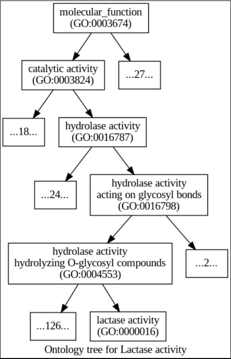
Figure 5.4 – An ontology tree for the “lactase activity” term (the terms at the top are more general); the top of the tree is molecular_function; for all ancestral nodes, the number of extra offspring is also noted (or enumerated, if less than three)
There’s more...
If you are interested in gene ontologies, your main port of call will be http://geneontology.org, where you will find much more information on this topic. Apart from molecular_function, gene ontology also has a biological process and a cellular component. In our recipes, we have followed the hierarchical relationship is a, but others do exist partially. For example, “mitochondrial ribosome” (GO:0005761) is a cellular component and is part of “mitochondrial matrix” (refer to http://amigo.geneontology.org/amigo/term/GO:0005761#display-lineage-tab and click on Graph Views).
As with the previous recipe, you can download the MySQL dump of a gene ontology database (you may prefer to interact with the data in that way). For this, see http://geneontology.org/page/download-go-annotations. Again, expect to allocate some time to understanding the relational database schema. Also, note that there are many alternatives to Graphviz for plotting trees and graphs. We will return to this topic later in this book.
See also
Here are some resources you can learn more from:
- As mentioned previously, more so than Ensembl, the main resource for gene ontologies is http://geneontology.org.
- For visualization, we are using the pygraphviz library, which is a wrapper on top of Graphviz ( http://www.graphviz.org).
- There are very good user interfaces for GO data, such as AmiGO (http://amigo.geneontology.org) and QuickGO (http://www.ebi.ac.uk/QuickGO/).
- One of the most common analyses performed with GO is gene enrichment analysis to check whether some GO terms are overexpressed or underexpressed in a certain gene set. The geneontology.org server uses Panther (http://go.pantherdb.org/), but other alternatives are available (such as DAVID, at http://david.abcc.ncifcrf.gov/).