
5
Filtering, Sorting, and Aggregations
In the last chapter, we looked at basic querying using Cypher. In this chapter, we will take it a step further by discussing adding filtering, sorting, and aggregations to the querying. We will cover these aspects in this chapter:
- Filtering with node labels and relationship types
- Filtering with WHERE and WITH clauses
- Sorting data using the ORDER BY clause
- Working with aggregations
We will start by filtering the data in queries.
Filtering with node labels and relationship types
In Cypher, filtering starts with the usage of node labels and relationship types. Let us take a look at a query where we do not apply any filters in Cypher:
MATCH p=()—-() RETURN p
This query returns all paths where any nodes are connected. In this query, there is no filtering. This query is shown to illustrate the fact that filtering is a bit different from SQL queries. Now, let us take a look at this query:
MATCH p=()—->() RETURN p
In this query, we are not using any node labels or relationship types, but we are filtering on relationships by outgoing direction:
MATCH p=(:Patient)—->() RETURN p
When we look at this query, we are looking for Patient nodes first and traversing all the outgoing relationships to find the paths. This showcases how node labels are leveraged for filtering:
MATCH p=(:Patient)-[:HAS_ZIPCODE]->() RETURN p
This query applies one more filter to the previous query. Now, we are only looking at outgoing HAS_ZIPCODE relationship types from Patient nodes and only returning those paths.
We will take a look at one of the queries we built in the previous chapter and see how adding labels and relationships to the path impacts the performance of the query. The query we are picking is the one where we look at the number of patients to which a drug has been prescribed:
MATCH (d:Drug)<-[:HAS_DRUG]-()<-[:HAS_ENCOUNTER]-(p)
WITH DISTINCT d, p
RETURN d.description as drug, count(p) as patients
In this query, we are starting from the Drug node and traversing an incoming HAS_DRUG relationship, ignoring the node label, traversing the HAS_ENCOUNTER relationship, and ignoring the label of the node coming next. Let us profile this query and see the performance of the query. The DISTINCT clause also acts as a filter in this query. If we have more than one prescription of the same drug for a patient, we want to count that as only one, so using DISTINCT here eliminates duplicates.
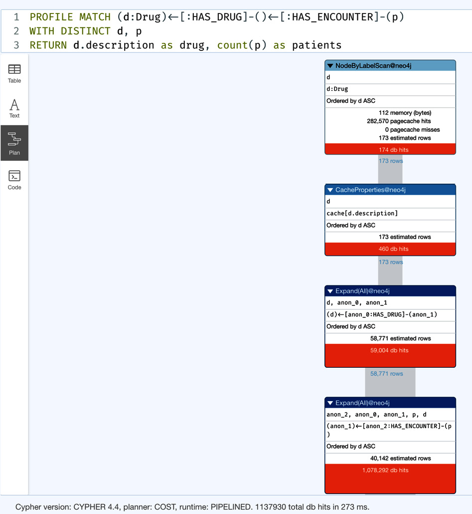
Figure 5.1 – Profile of drug-patient interactions – iteration 1
We can see that it generates 1,137,930 db hits.
Now, let us look at the same query – most developers are going to write it as follows:
MATCH (d:Drug)<-[:HAS_DRUG]-(e:Encounter)<-[:HAS_ENCOUNTER]-(p:Patient)
WITH DISTINCT d, p
RETURN d.description as drug, count(p) as patients
One difference we see in the query here is that we have added labels and variables for intermediate nodes where we used to ignore the labels. Let us look at this query’s performance:
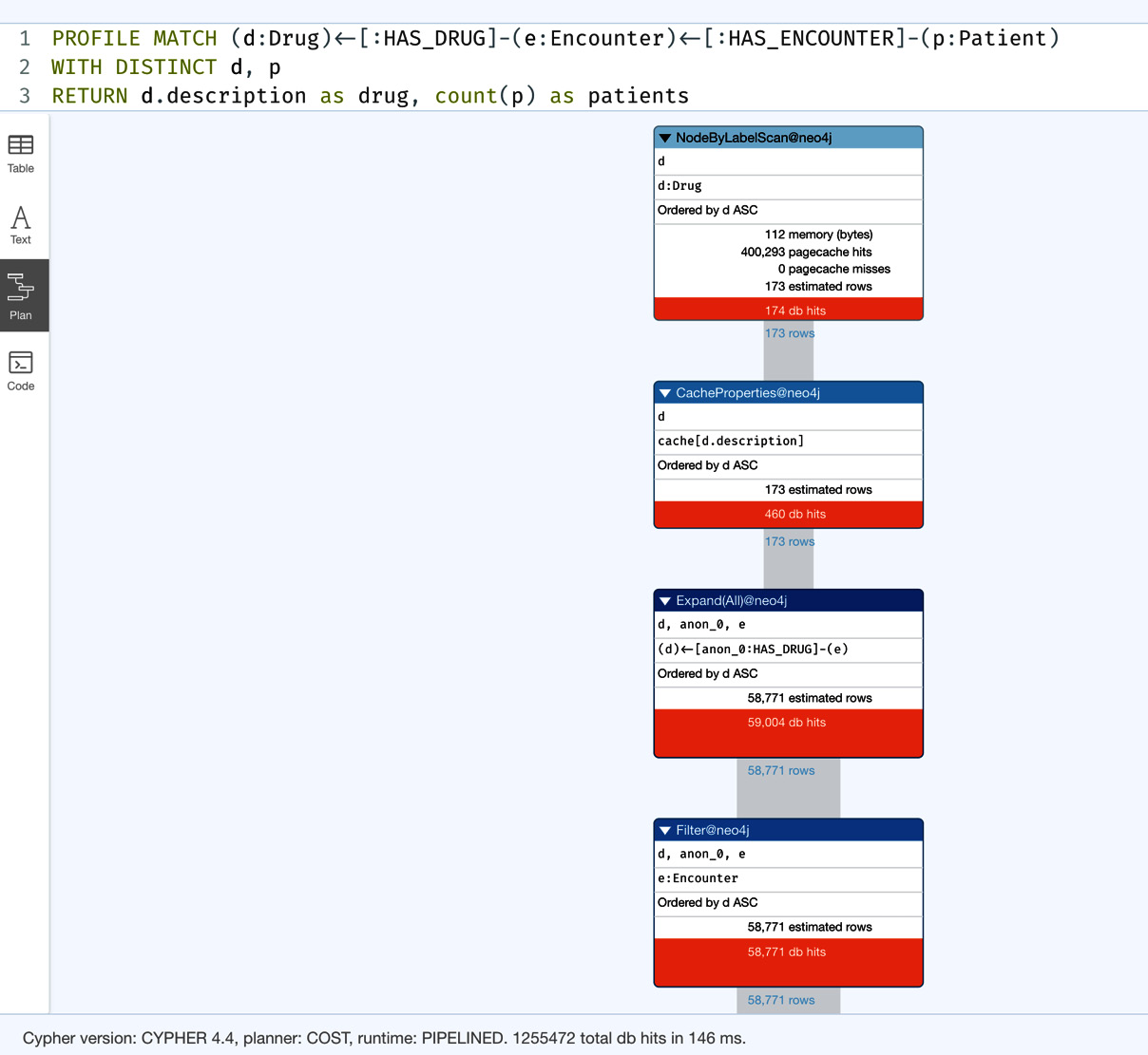
Figure 5.2 – Profile of drug-patient interactions – iteration 2
We can see that this query generates 1,255,472 db hits, which is 11% more than the previous iteration, where we didn’t specify labels for more strict filtering. This is a bit counterintuitive for SQL developers. This is because of the way Neo4j processes the query. Neo4j optimizes the traversal patterns. When we add a label to a node in the traversal, then Neo4j must stop there and check whether the node in the path has that label. This is one extra db hit. This is why this query requires more database work to complete the query while making the most sense from a filtering perspective.
Here’s another iteration of the same query that most SQL developers would write when migrating to graph databases:
MATCH (d:Drug)<--(e:Encounter)<--(p:Patient)
WITH DISTINCT d, p
RETURN d.description as drug, count(p) as patients
In this query, we can see the developer relying on node labels that are connected to others ignoring the relationship types. Let us look at the performance of this query:
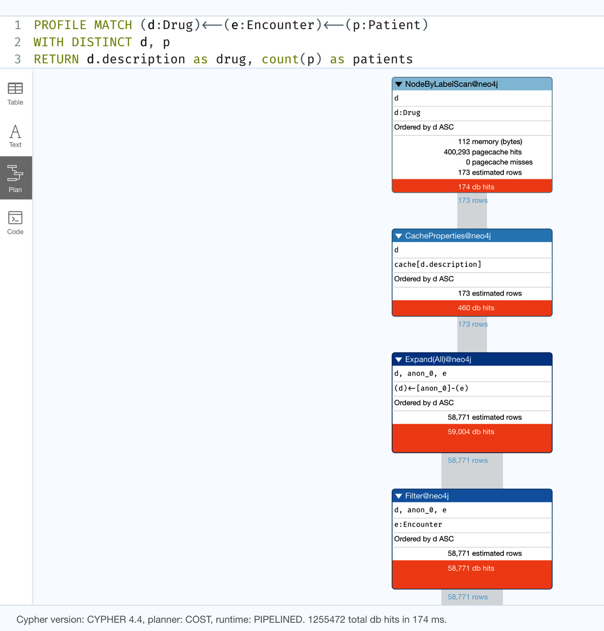
Figure 5.3 – Profile of drug-patient interactions – iteration 3
We can see this version of the query generates 1,255,472 db hits. This is the same as the previous revision of the query. This is because both Drug and Encounter nodes only have one type of incoming relationship. So, in this case, there is no difference in the performance whether we specify the relationship type or not.
Now, let us take a look at another version of the same query that most SQL developers would write:
MATCH (d:Drug)--(e:Encounter)--(p:Patient)
WITH DISTINCT d, p
RETURN d.description as drug, count(p) as patients
The difference in the query here is that the direction of the relationship is taken out. This is one of the most common query patterns that new developers would attempt to write. Let us look at the performance of this query:
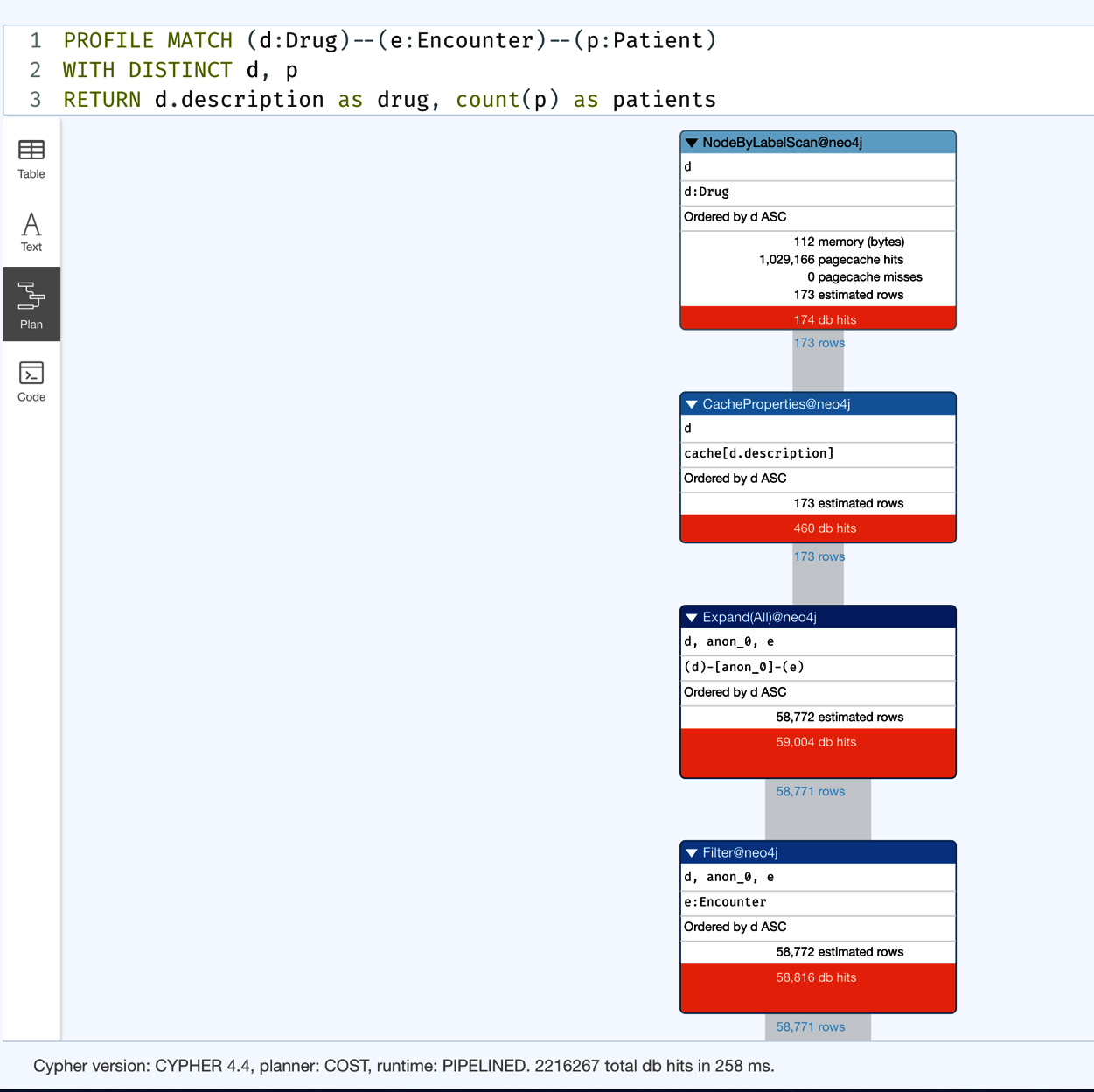
Figure 5.4 – Profile of drug-patient interactions – iteration 4
We can see this query is taking 2,216,267 db hits. This is 80% more db hits than the last version and almost double the number of db hits when compared to the original version of the query.
From these queries, we can see that node labels and relationship types can act as filters in the query, unlike in SQL, where only the WHERE clause is used for filtering or JOINS. Another aspect we can notice here is that using relationship types and the direction of the relationship in the query is more performant than using node labels.
Tip
When a relationship type uniquely identifies the start or end node types, then not providing labels in the traversal can improve the query performance. The only place we should use a label is when we are using a WHERE condition and want to leverage indexes or a relationship type is not enough.
Now, let us look at filtering the data using WHERE and WITH clauses.
Filtering with WHERE and WITH clauses
Now, let us build on the previous query and say we only want to return drugs that have more than 100 patients associated with them. This is the scenario in which the WHERE clause would come into the picture.
The Cypher query looks like this:
MATCH (d:Drug)<-[:HAS_DRUG]-()<-[:HAS_ENCOUNTER]-(p)
WITH DISTINCT d, p
WITH d.description as drug, count(p) as patients
WHERE patients > 100
RETURN drug, patients
To achieve what we want, we changed the query as shown in the highlighted section. We have to use the WITH clause first to collect the data and then apply a filter using the WHERE clause to prevent the data from being returned:
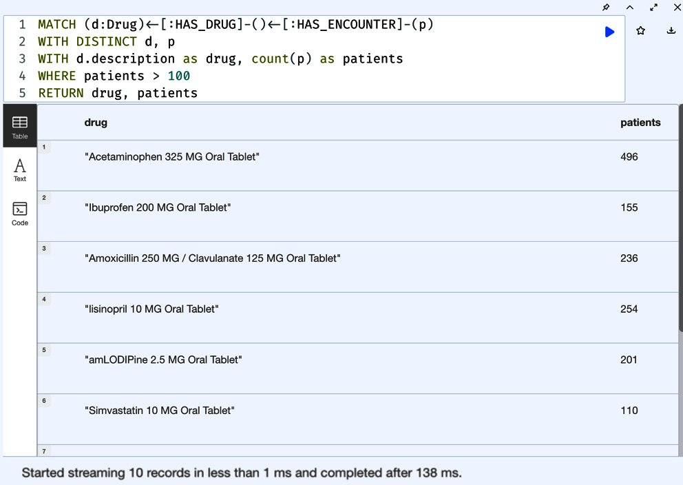
Figure 5.5 – Drugs with more than 100 patients associated with them
The preceding screenshot shows the response. We can see there are only 10 drugs that have more than 100 patients who have a prescription for them.
We can also use SKIP and LIMIT to filter the data being returned. Say we only wanted to return 20 records from the drug prescriptions query – it would look like this:
MATCH (d:Drug)<-[:HAS_DRUG]-()<-[:HAS_ENCOUNTER]-(p)
WITH DISTINCT d, p
RETURN d.description as drug, count(p) as patients
LIMIT 20
This is the same as the original drug interaction query. The only change we have made is to add a LIMIT clause to the end to limit the number of results.
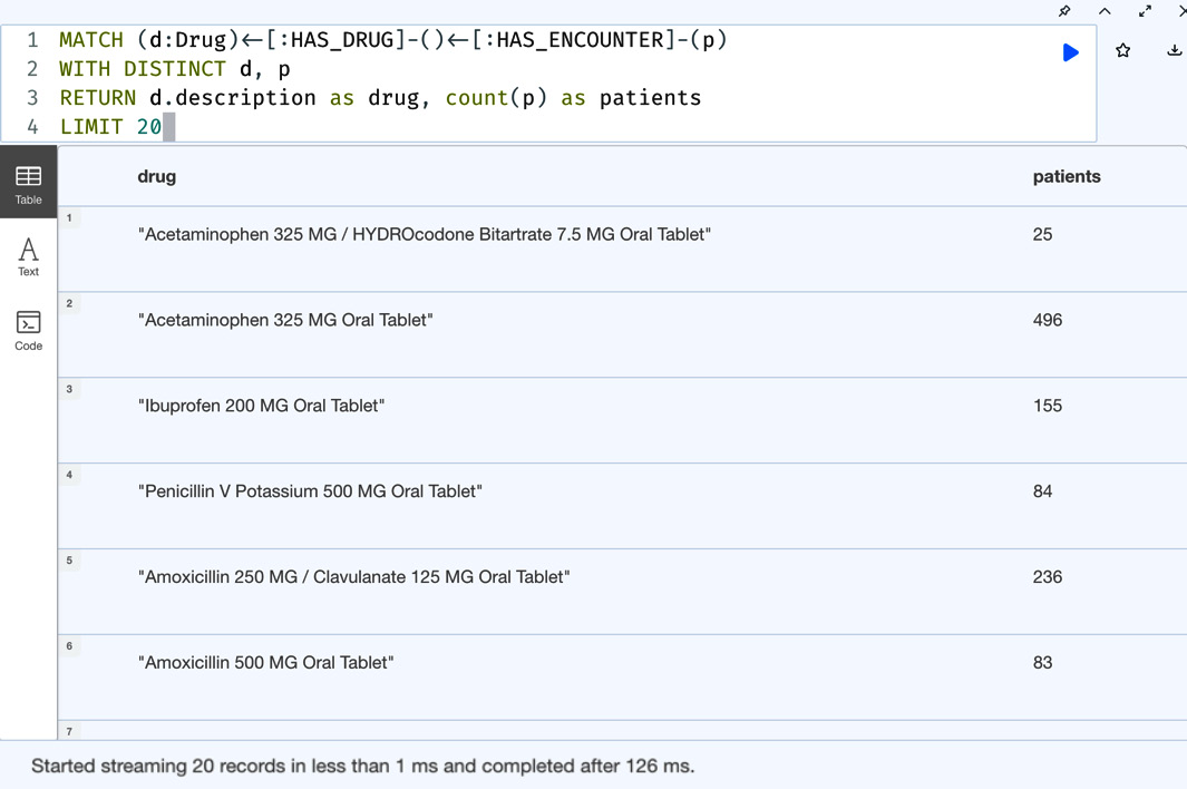
Figure 5.6 – First 20 records of drugs with the patients associated with them
We can see in the response that we got exactly 20 records. If the response data has less than 20 records, then all the records would be returned.
Similarly, we can use the SKIP clause to skip the initial records. Let us take a look at the query to skip the first 20 records and return the remaining data:
MATCH (d:Drug)<-[:HAS_DRUG]-()<-[:HAS_ENCOUNTER]-(p)
WITH DISTINCT d, p
RETURN d.description as drug, count(p) as patients
SKIP 20
This query will skip the first 20 records and return the remaining data:
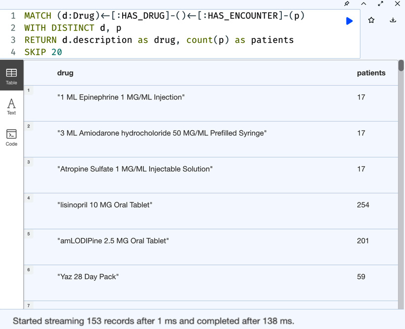
Figure 5.7 – Skipping the first 20 records of drugs and the patients associated with them
We can see we have 153 more records of data that are returned after skipping the first 20 records. If the original data set had less than 20 records, then no data would be returned.
We can also combine SKIP and LIMIT to skip the first few records and then limit the next set of records.
In this case, the query looks like this:
MATCH (d:Drug)<-[:HAS_DRUG]-()<-[:HAS_ENCOUNTER]-(p)
WITH DISTINCT d, p
RETURN d.description as drug, count(p) as patients
SKIP 20
LIMIT 20
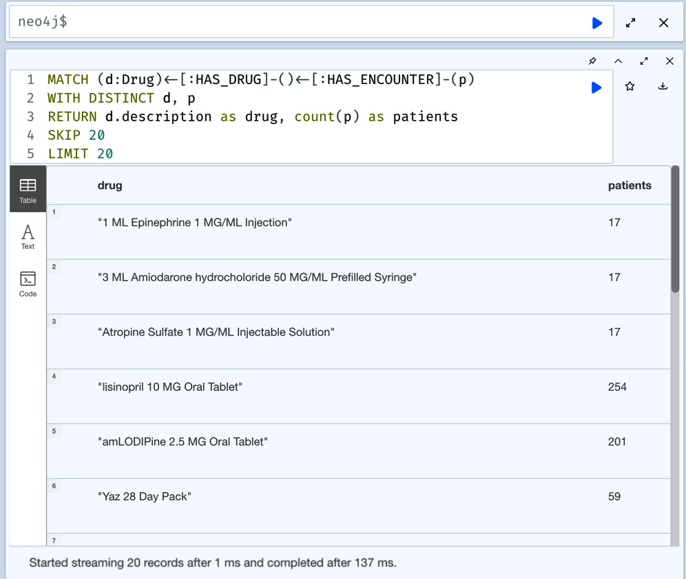
Figure 5.8 – Skipping the first 20 records and returning the next 20 records of drugs with the patients associated with them
We can see here that 20 of the 153 records are returned from the previous query. It is possible to use SKIP and LIMIT to paginate the response. One thing we need to understand here is that the query execution time may not differ much from the full query and should be used with care. Let us look at the profile of this query to understand the db hits:
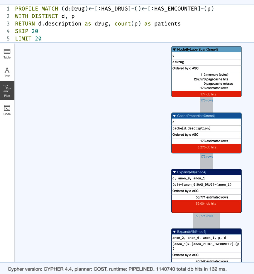
Figure 5.9 – Query profile with SKIP and LIMIT
We can see that the query generates 1,140,740 db hits, which is slightly higher than the db hits for the original query. It seems the LIMIT clause is adding a few extra db hits in terms of performance. This is why when we are thinking of pagination using SKIP and LIMIT, we need to take a holistic approach to the overall performance of the system rather than forcing pagination at the database level.
For filtering, along with the WHERE clause, we can also use an EXISTS or NOT EXISTS clause to filter data. We can use an EXISTS clause to check whether a pattern exists or a property exists for a node or a relationship. Let us count the encounter nodes that do have an end date property.
The Cypher code for this looks like this:
MATCH (e:Encounter)
WHERE EXISTS(e.end)
RETURN count(e)
This returns the number of encounters that have the end property:
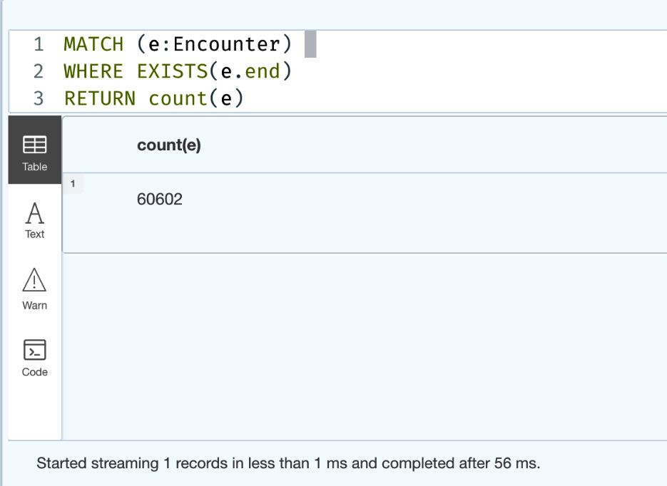
Figure 5.10 – Query using the EXISTS property
When we try this in the browser, it gives a warning that the use of EXISTS is deprecated for property checking. The supported way of doing this in Cypher is shown here:
MATCH (e:Encounter)
WHERE e.end IS NOT NULL
RETURN count(e)
This is the supported usage of checking whether a property exists in future versions of Cypher.
Let us see the usage of NOT EXISTS with a pattern check. Let us find patients that do not have a ZIP code associated with them. The Cypher code for this looks like this:
MATCH (p:Patient)
WHERE NOT EXISTS ((p)-[:HAS_ZIPCODE]->())
RETURN p
LIMIT 5
We can see in this query that we are checking for the absence of the ((p)-[:HAS_ZIPCODE]->()) pattern and returning the five patients that match this condition:
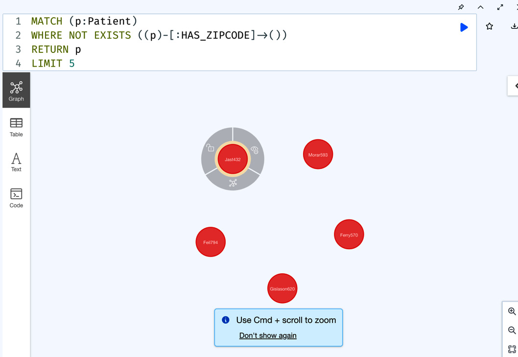
Figure 5.11 – Query using a NOT EXISTS pattern
We can see from the results that we are seeing patients who do not have ZIP codes associated with them. We can also use regular expressions in the WHERE clause to find data. Let’s find patients whose first name starts with Jas using a regular expression. The Cypher query for this looks like this:
MATCH (p:Patient)
WHERE p.firstName =~'Jas.*'
RETURN p.firstName
This query finds all the patients whose first name starts with Jas and returns those first names.
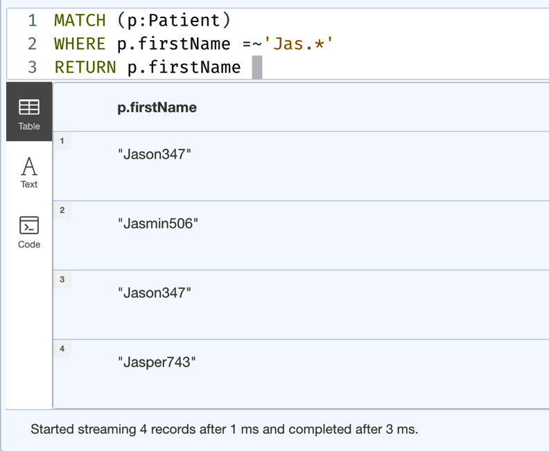
Figure 5.12 – Query using a regular expression
From the screenshot, we can see the response that matches the regular expression.
Now, let us look at sorting the results after filtering.
Sorting data using the ORDER BY clause
We can sort the results using the ORDER BY clause. Let us take the drug prescription query and apply sorting to it. First, let us take a look at the query that sorts results by the number of patients to which they are prescribed:
MATCH (d:Drug)<-[:HAS_DRUG]-()<-[:HAS_ENCOUNTER]-(p)
WITH DISTINCT d, p
RETURN d.description as drug, count(p) as patients
ORDER BY patients
This query returns the drug prescriptions in ascending order based on the number of patients they are prescribed to.
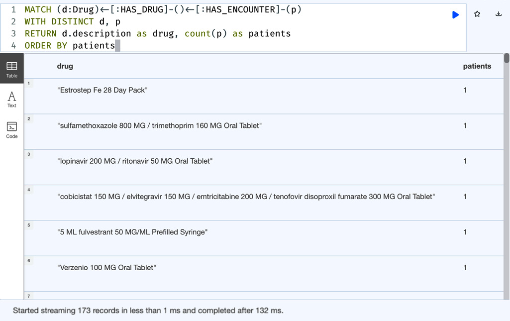
Figure 5.13 – Drug prescriptions ordered by the number of patients they are prescribed to
We can see the data in ascending order based on the number of patients the drugs are prescribed to. Now, let us look at the query where the data is in descending order:
MATCH (d:Drug)<-[:HAS_DRUG]-()<-[:HAS_ENCOUNTER]-(p)
WITH DISTINCT d, p
RETURN d.description as drug, count(p) as patients
ORDER BY patients DESC
Let us take a screenshot of the query results:
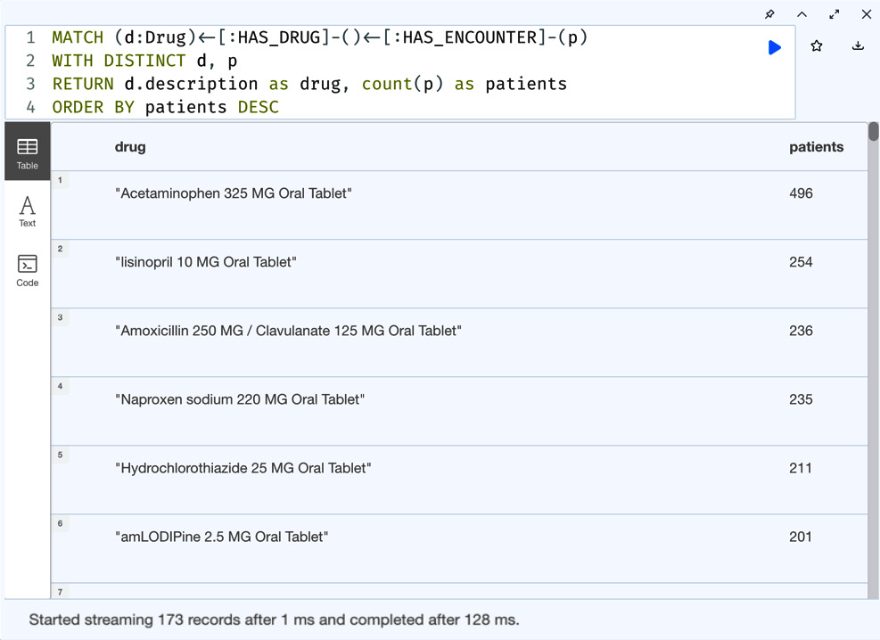
Figure 5.14 – Drug prescriptions in descending order by the number of patients they are prescribed to
We can see from the screenshot that the data is in descending order based on the number of patients the drug is prescribed to.
Now, let us take a look at another query. We will write a query to retrieve the top 10 drugs prescribed based on the number of patients they are prescribed to. The Cypher code looks like this:
MATCH (d:Drug)<-[:HAS_DRUG]-()<-[:HAS_ENCOUNTER]-(p)
WITH DISTINCT d, p
RETURN d.description as drug, count(p) as patients
ORDER BY patients DESC
LIMIT 10
This query returns the top 10 drugs prescribed.
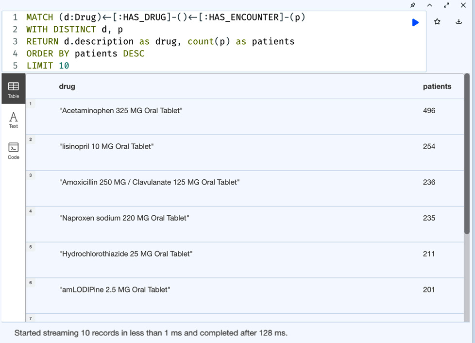
Figure 5.15 – Top 10 drugs prescribed
The screenshot shows the top 10 drugs prescribed. Now, let us add a filter to sort queries. Let us get the first 10 drugs prescribed that have been prescribed to at least 50 patients and order them by the number of patients.
The Cypher query looks like this:
MATCH (d:Drug)<-[:HAS_DRUG]-()<-[:HAS_ENCOUNTER]-(p)
WITH DISTINCT d, p
WITH d.description as drug, count(p) as patients
WHERE patients > 50
RETURN drug, patients
ORDER BY patients
LIMIT 10
We can see in the query that the patients count filter is added before returning the data sorted in ascending order.
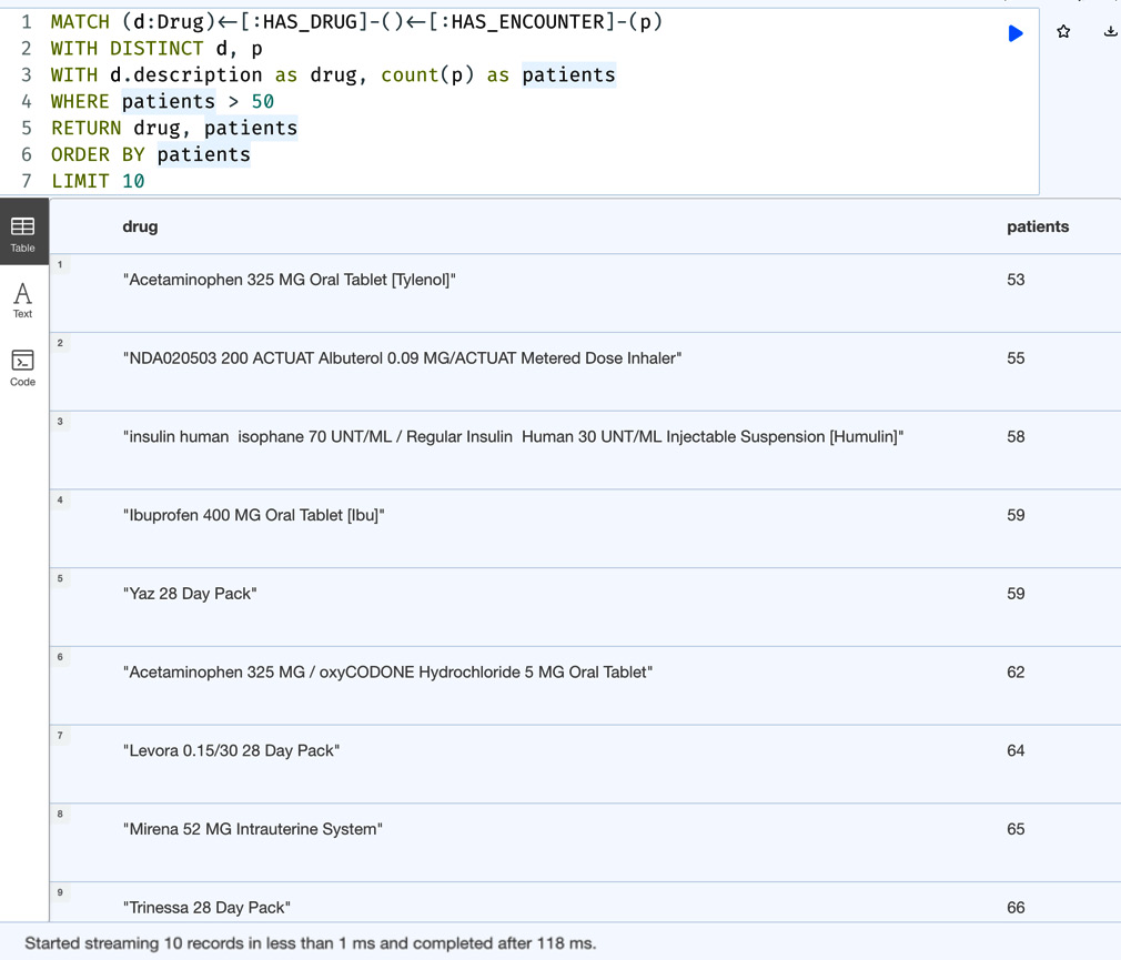
Figure 5.16 – Bottom 10 drugs prescribed with at least 50 patients
We can see from the result set that we are getting drugs that have more than 50 patients associated with them.
We can apply the ORDER BY clause first before applying the filter. The Cypher query looks like this:
MATCH (d:Drug)<-[:HAS_DRUG]-()<-[:HAS_ENCOUNTER]-(p)
WITH DISTINCT d, p
WITH d.description as drug, count(p) as patients
ORDER BY patients
WITH drug, patients
WHERE patients > 50
RETURN drug, patients
LIMIT 10
We can see from the query that we are applying the ORDER BY clause first and then applying the patients > 50 filter after that.
Let us take a look at the results to see whether they are the same:
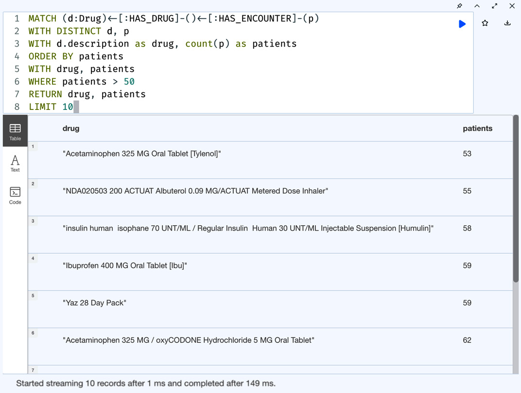
Figure 5.17 – Bottom 10 drugs prescribed with at least 50 patients – ORDER BY first
We can see that the response is the same in both cases. We have seen ORDER BY with one property. Let us try the query with multiple properties in the ORDER BY clause. Let us sort the data by the drug name and patient count first. The Cypher query looks like this:
MATCH (d:Drug)<-[:HAS_DRUG]-()<-[:HAS_ENCOUNTER]-(p)
WITH DISTINCT d, p
WITH d.description as drug, count(p) as patients
WHERE patients > 100
RETURN drug, patients
ORDER BY  drug, patients
LIMIT 10
In this query, we are using the drug name as the primary sorting point and the patient count as the secondary sorting point.
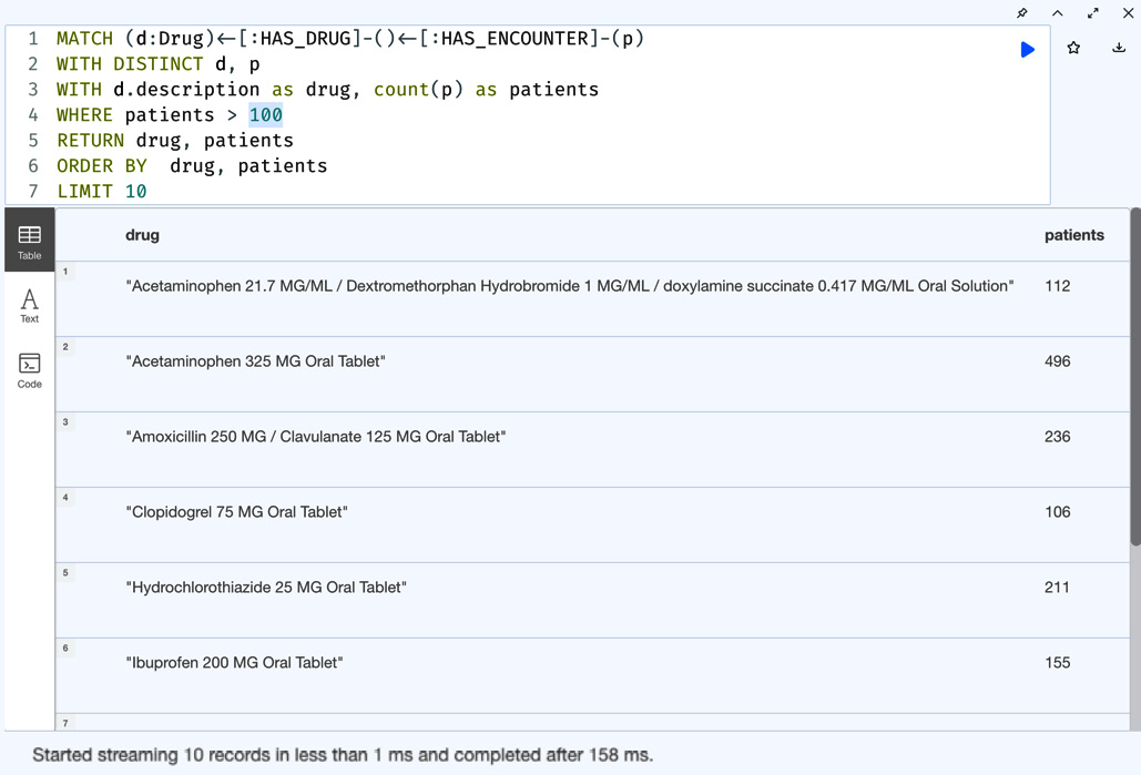
Figure 5.18 – Bottom 10 drugs prescribed – ordered by drug name and patient count
We can see here both the drug name and patient count are used for sorting. Let us change the primary and secondary sorting points to the patient count and drug name.
The Cypher query for this looks like this:
MATCH (d:Drug)<-[:HAS_DRUG]-()<-[:HAS_ENCOUNTER]-(p)
WITH DISTINCT d, p
WITH d.description as drug, count(p) as patients
WHERE patients > 100
RETURN drug, patients
ORDER BY patients, drug
LIMIT 10
In this query, we are using the patient count as the primary sorting point and the drug name as the secondary sorting point.
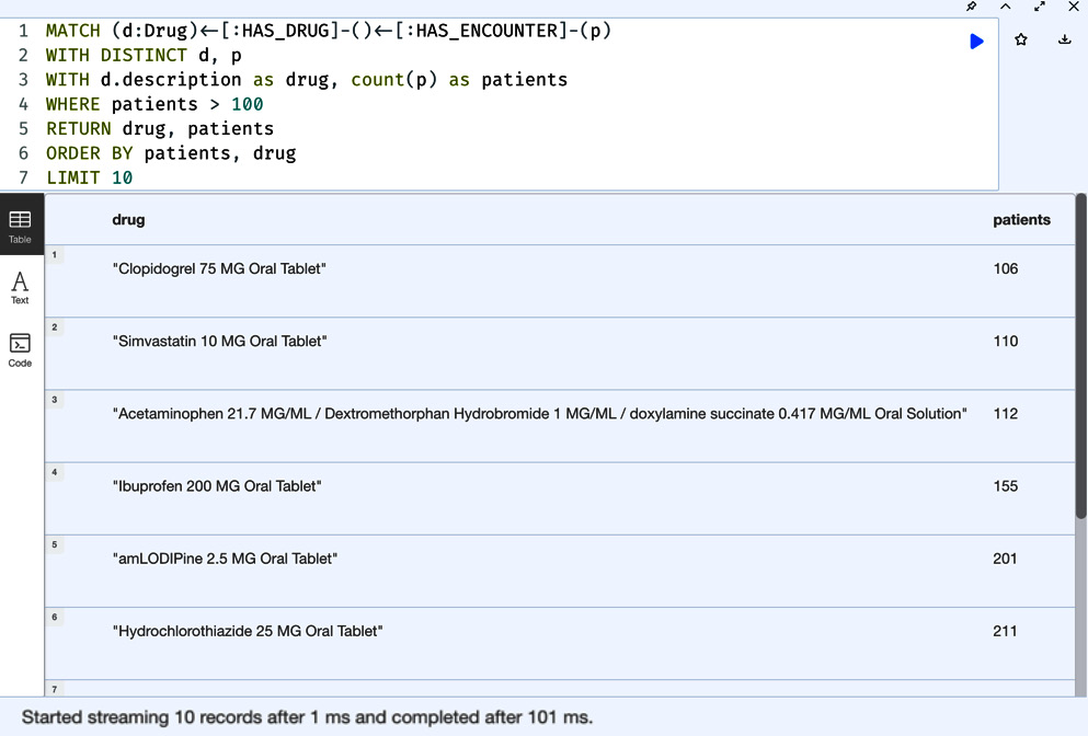
Figure 5.19 – Bottom 10 drugs prescribed – ordered by patient count and drug name
We can see the sorted results changed from the previous query. When we have multiple properties, we can change the order of sorting per field. Let us take a look at the drug name descending as the primary sorting point and the patient count ascending as the secondary point.
The Cypher query in this case looks like this:
MATCH (d:Drug)<-[:HAS_DRUG]-()<-[:HAS_ENCOUNTER]-(p)
WITH DISTINCT d, p
WITH d.description as drug, count(p) as patients
WHERE patients > 100
RETURN drug, patients
ORDER BY  drug DESC, patients
LIMIT 10
Here, we are using drug names descending as the primary sorting point and patient counts ascending as a secondary sorting point:
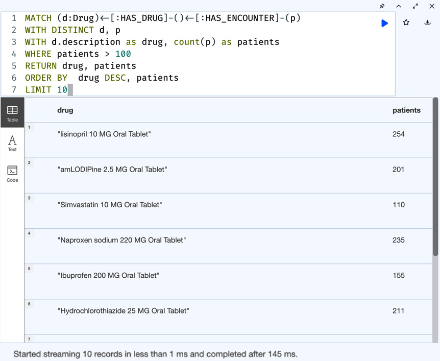
Figure 5.20 – Drug prescriptions – ordered by drug names in descending order and patient counts in ascending order
We can see from the screenshot that the drug names are in descending order and the patient counts are in ascending order. Let us add descending order for both properties:
MATCH (d:Drug)<-[:HAS_DRUG]-()<-[:HAS_ENCOUNTER]-(p)
WITH DISTINCT d, p
WITH d.description as drug, count(p) as patients
WHERE patients > 100
RETURN drug, patients
ORDER BY  drug DESC, patients DESC
LIMIT 10
In this query, we are sorting data by both sorting points in descending order.
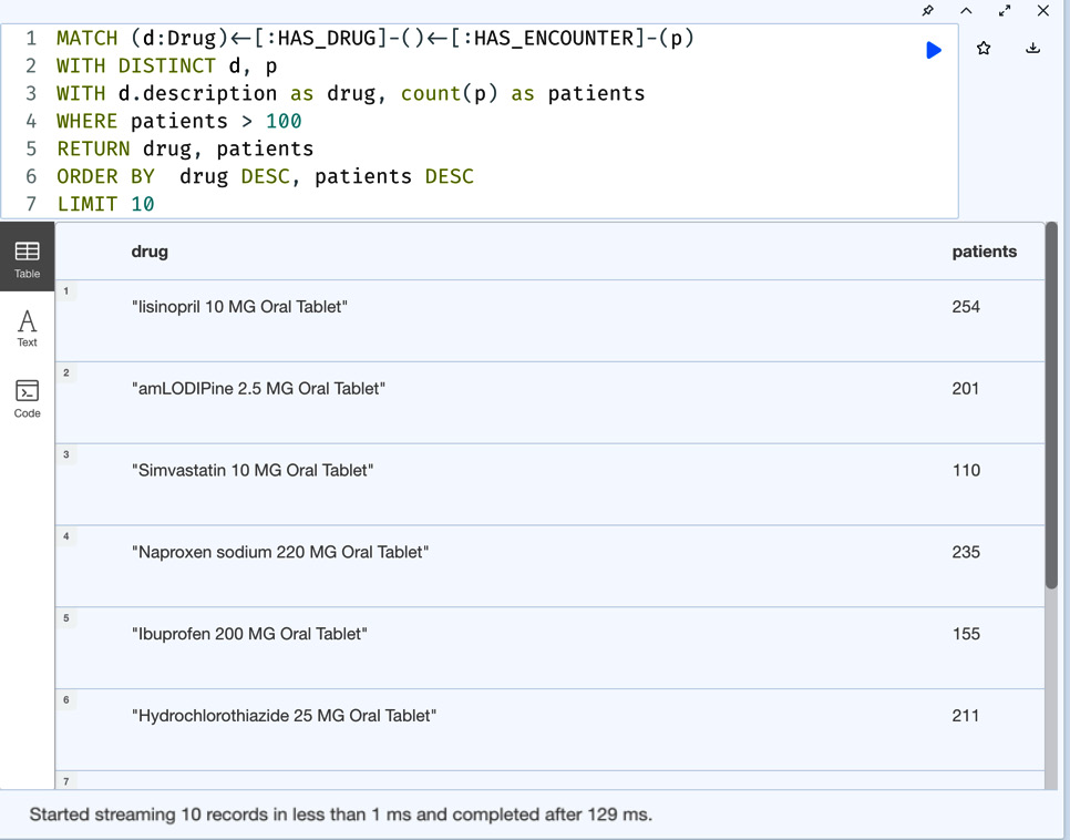
Figure 5.21 – Drug prescriptions – ordered by drug names in descending order and patient counts in descending order
The data seems the same as the query before because of the way the data is distributed. The drug name order causes the response to be similar to the other query.
Now that we have worked with filtering and sorting data, let us take a look at working with aggregations.
Working with aggregations
In Cypher, aggregations are supported using the COUNT, SUM, AVG, MIN, MAX, COLLECT, PERCENTILE, and STDEV functions. Except for the COLLECT function, all the other functions are standard mathematical functions. COLLECT functions create a list of entities similar to data pivoting by converting a list of rows into a column value.
We have seen the usage of the COUNT function numerous times in this chapter. We can combine COUNT and COLLECT to count the entities as well as collect the values as a list. Let us take a look at the drug prescription query where we were returning patient counts. We will also return the first names of those patients along with the count.
For this, the Cypher query looks like this:
MATCH (d:Drug)<-[:HAS_DRUG]-()<-[:HAS_ENCOUNTER]-(p)
WITH DISTINCT d, p
WITH d.description as drug,
     COUNT(p) as patients,
     COLLECT(p.firstName) as firstNames
WHERE patients > 10
RETURN drug, patients, firstNames
ORDER BY patients
LIMIT 10
In this query, we are returning the drug name and patient count where the patient count is more than 10 along with the first names of those patients. We can see here we are combining the COUNT and COLLECT functions together. In Cypher, when we are doing aggregations, the group-by functionality is automatic, unlike SQL. It will group by all the values that are not part of COUNT or COLLECT:
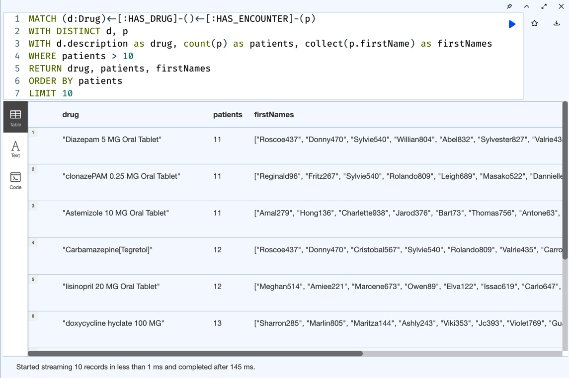
Figure 5.22 – Drug prescriptions – COUNT and COLLECT usage
We can see in the screenshot we are seeing the patient count as well as the patients’ first names. Since lists are first-class citizens in Cypher, it is easier to pivot the data from rows into columns.
Now, let us take a look at the same drug interaction query, with patient MIN, MAX, and AVG ages instead of first names.
The Cypher query for this looks like this:
MATCH (d:Drug)<-[:HAS_DRUG]-()<-[:HAS_ENCOUNTER]-(p)
WHERE p.birthDate IS NOT NULL
WITH DISTINCT d, p
WITH d, p, duration.between(p.birthDate, date()).years as age
WITH d.description as drug,
     count(p) as patients,
     min(age) as minAge,
     max(age) as maxAge,
     avg(age) as avgAge
WHERE patients > 25
RETURN drug, patients, minAge, maxAge, avgAge
ORDER BY patients
LIMIT 20
First, this query only selects the patients for whom we have a birth date. Once we have found the patients, we use the duration function to calculate the age of the patient. Once have we calculated the age, while counting the number of patients for that group of patients, we calculate the minimum, maximum, and average age using aggregation functions. For more documentation on the usage of duration, please visit the Durations documentation: https://neo4j.com/docs/cypher-manual/current/syntax/temporal/#cypher-temporal-durations.
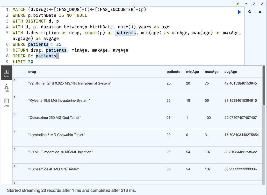
Figure 5.23 – Drug prescriptions – MIN, MAX, and AVG usage
We can see from the screenshot we get the minimum, maximum, and average ages of the patients associated with the drug.
Summary
In this chapter, we looked at building queries while applying filters. We have taken a look at filtering the data using node labels and relationship types, using relationship directions, the performance impact of using node labels when compared to relationship types for traversal, using WHERE clauses, WITH clauses, SKIP clauses, LIMIT clauses, and EXISTS clauses, and using regular expressions.
We looked at sorting the data using the ORDER BY clause with one value or multiple values in ascending order or in descending order and combining the ORDER BY clause with the WITH clause.
Finally, we looked at aggregating results using the COUNT, COLLECT, MIN, MAX, and AVG functions. Along with this, we also looked at combining the COUNT and COLLECT functions to perform some complex aggregations.
In the next chapter, we will take a look at using LIST expressions, working with the UNION clause. We will also take a look at using sub-queries using the CALL clause.