8

Advanced Query Patterns

In the last chapter, we looked at working with lists and maps. In this chapter, we will explore some advanced query patterns using Cypher clauses. We will discuss query chaining using the WITH clause, iterate lists to modify the graph using the FOREACH and UNWIND clauses, and leverage count stores for building optimal queries. We will also take a look at simulating if condition using the FOREACH clause. We will take a deeper look at these clauses and discuss how they can help us in building more advanced and complex queries.

In this chapter, we will be covering the following aspects:

• Working with the WITH clause
• Working with the CASE clause
• Working with the FOREACH clause
• Working with the UNWIND clause
• Working with count stores

First, we will start by exploring the WITH clause. This is a very powerful paradigm that helps us build complex and performant queries with ease.

Working with the WITH clause

In Cypher, the WITH clause allows individual queries to be chained together by streaming the results from the first part of the query to the next part of the query. It allows you to manipulate the query result before it is passed on to the next part of the query.

We will take a look at different ways in which we can work with the WITH clause. We will start by introducing the variables at the beginning of the Cypher query.

Introducing variables at the start

When a query starts with the WITH clause, we need to introduce the variables for the next part of the query.

Let’s look at an example:

WITH range(1,5,1) as list
RETURN list

In this query, we are introducing a variable called list and returning it.

The following screenshot shows how to prepare a new variable using the WITH clause and return values based on that variable.

Figure 8.1 – Basic WITH usage introducing a new variable at the start

Now, let’s look at using the new variable defined to perform MATCH:

WITH '313820' as code
MATCH (d:Drug {code:code})
RETURN d

In this query, we are defining a new variable using the WITH clause and then using that variable to perform other tasks in the next part of the query.

The following screenshot shows that we can retrieve the node by referring to the variable defined using the WITH clause.

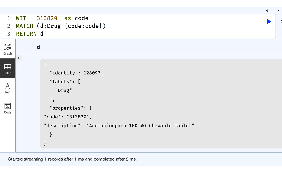
Figure 8.2 – Using a new variable to perform MATCH in the next part of the query

Now, let’s look at getting some data in the first part of the query and passing it to the next part of the query:

MATCH (p:Patient {ssn:'999-10-9496'})-[:HAS_ENCOUNTER]->()-[:HAS_DRUG]->(d:Drug)
WITH d
RETURN d.code, d.description

In this code, we are performing a MATCH query to get a Patient node and all the drugs they are prescribed in the first part of the query, and then we are passing only the drug nodes we found in this part of the query to the next query.

From the following screenshot, we can see that we are getting all the drug values with the RETURN clause using the variable passed with the WITH clause. We need to remember that all the other variables in the first part of the query are not available in the next part of the query.

Figure 8.3 – Passing variables from one part of the query to another

Let us see what happens when we try to use the variables defined in the first part of the query in the second part of the query:

MATCH (p:Patient {ssn:'999-10-9496'})-[:HAS_ENCOUNTER]->()-[:HAS_DRUG]->(d)
WITH d
RETURN p.ssn, d.code, d.description

This query tries to access the Patient node in the second part of the query that was retrieved in the first part of the query.

As we can see from the following screenshot, we get an error saying that the variable is not defined. This is because the WITH clause defines a new scope and only the variables passed using that clause are available in the new scope of the second part of the query.

Figure 8.4 – Using a variable in the second part of the query not passed using WITH

Say we want to pass all the variables we have retrieved in the first part of the query to the second part of the query without referring to each of them manually; we can use a wildcard, *, to do that. Let’s look at how this is done:

MATCH (p:Patient {ssn:'999-10-9496'})-[:HAS_ENCOUNTER]->()-[:HAS_DRUG]->(d)
WITH *
RETURN p.ssn, d.code, d.description

In this query, we are passing all the variables we have defined in the first part of the query to the second part of the query.

As we can see from the following screenshot, there are no more errors now. Data is returned from the query.

Figure 8.5 – Passing all the variables from the first part of the query to the second using a wildcard

Using the WITH clause, we can not only return the variables from the first part of the query, but we can introduce new variables using aggregate functions, such as count and collect, or other clauses.

Let’s take a look at a query that uses aggregation functions as well as the WITH clause:

MATCH (p:Patient {ssn:'999-10-9496'})-[:HAS_ENCOUNTER]->()-[:HAS_DRUG]->(d)
WITH d, count(d) as prescriptions
RETURN d.code, d.description, prescriptions

This query returns the drug code, name, and the number of times it has been prescribed for the given patient. We can see that we have introduced a new variable called prescriptions by using the count method.

From the following screenshot, we can see that we are getting the distinct drug codes and names, along with the number of times the drug has been prescribed to this patient.

Figure 8.6 – Introducing a new variable along with an existing variable

Along with the new variables, we can also introduce a WHERE condition to continue to the next part of the query only when certain conditions have been met. Let’s look at an example of this:

MATCH (p:Patient {ssn:'999-10-9496'})-[:HAS_ENCOUNTER]->()-[:HAS_DRUG]->(d)
WITH d, count(d) as prescriptions
WHERE prescriptions > 10
RETURN d.code, d.description, prescriptions

In this query, we are trying to return only the drugs that have been prescribed more than 10 times.

From the following screenshot, we can now see that only two drugs have been prescribed more than 10 times.

Figure 8.7 – Adding a WHERE clause along with new variables

We can also apply ORDER BY to the first part of the query result set along with the WITH clause before processing them in the next part of the query. Let’s look at an example of this:

MATCH (p:Patient {ssn:'999-10-9496'})-[:HAS_ENCOUNTER]->()-[:HAS_DRUG]->(d)
WITH d, count(d) as prescriptions
ORDER BY d.code
RETURN d.code, d.description, prescriptions

In this query, we are ordering the first query results by drug code and then passing the results to the next part of the query.

Let’s execute the query and review the results.

Figure 8.8 – Applying ORDER BY to the first part of the query results and passing them on to the next part

We can see from the screenshot that the response has now ordered the results by drug code. It is also possible to apply the LIMIT clause to the first part of the query results. Let’s look at this in the following code block:

MATCH (p:Patient {ssn:'999-10-9496'})-[:HAS_ENCOUNTER]->()-[:HAS_DRUG]->(d)
WITH d, count(d) as prescriptions
ORDER BY d.code
LIMIT 4
RETURN d.code, d.description, prescriptions

Here, we are limiting the results from the first part of the query to 4, using these four results, and returning the required data in the next part of the query.

As we can see from the following screenshot, we are only getting the first four results from the ordered data from the first part of the query.

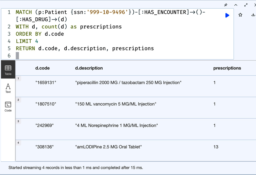
Figure 8.9 – Limiting the results from the first part of the query

Similarly, it is also possible to apply the SKIP clause and a combination of the SKIP and LIMIT clauses to the result set.

It is also possible to take the results from the first query and perform a different set of queries to do something completely different. Let’s take a look at this:

WITH '999-10-9496' as ssn
MATCH (p:Patient {ssn:ssn})-[:HAS_ENCOUNTER]->()-[:HAS_DRUG]->(d)
WITH d, count(d) as prescriptions
WHERE prescriptions > 10
MATCH (other)-[:HAS_ENCOUNTER]->()-[:HAS_DRUG]->(d)
WITH  other, d, count(d) as otherPrescriptions
WHERE otherPrescriptions > 10
RETURN other.ssn as otherPatients, d.code as drug, d.description as name, otherPrescriptions

In this query, we are finding the most prescribed drugs for the given patient and finding other patients to whom these drugs were prescribed most.

We can see from the following screenshot that we are able to branch after the first part of the query using the most prescribed drug node, which is passed to the second part of the query, which is retrieving the other patients who also had these drugs prescribed often. Another aspect we can notice is that we can keep the WITH chain going. In the previous query, we used WITH four times to keep passing the data to the next step while filtering for the desired results.

Figure 8.10 – Branching path in the second part of the query using WITH

In this section, we have discussed various ways to use the WITH clause to build advanced cypher queries. We will take a look at the CASE WHEN clause next and review various usage scenarios for building queries.

Working with the CASE clause

The CASE clause is an expression constructed that is used to transform results. There are two different forms of CASE expression and they are as follows:

• A simple CASE form to compare against multiple values
• A generic CASE form to express multiple conditional expressions

We will take a look at the simple CASE expression first.

Working with simple CASE expressions

In simple CASE expressions, the expression is evaluated and compared to the WHEN clauses. The corresponding expression is then evaluated and the resulting value is returned. If no value is found, the ELSE clause expression is evaluated and the corresponding value is returned. If there is no ELSE clause, then a null value is returned.

The syntactic representation of this looks like this:

CASE test
  WHEN value THEN result
  [WHEN ...]
  [ELSE default]
END

We can see from this syntax that the first CASE expression is evaluated and its value is compared to the WHEN clause. We can describe each variable or argument in this syntax in the following way:

• test – A valid expression. This can be evaluated into different values based on the data.
• value – An expression that will be compared against test.
• result – The value we want to return if value matches test.
• default – The value that will be returned when none of the value expressions match test.

Let’s take a look at an example usage:

MATCH (p:Patient)
RETURN p.ssn as patient, CASE p.marital
    WHEN "S" THEN "Single"
    WHEN "M" THEN "Married"
    ELSE "UNKNOWN"
END as status

In this query, we are getting all the patients’ statuses based on the marital property code and then returning an elaborate string as the response.

As we can see from the following screenshot, we are getting detailed text as the statuses instead of code.

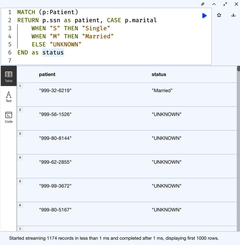
Figure 8.11 – Simple CASE expression

It is also possible to combine the WITH clause and apply the CASE expression after filtering data. Let’s look at an example usage of this:

MATCH (p:Patient)
WITH p.ssn as patient, CASE p.marital
    WHEN "S" THEN "Single"
    WHEN "M" THEN "Married"
    ELSE "UNKNOWN"
END as status
WHERE p.marital IS NOT NULL
RETURN patient, status

In this query, we are combining the CASE expression and the WITH clause and retrieving only those patients’ statuses who have a certain value for the marital property.

We can see from the following screenshot that we are not getting the UNKNOWN value returned anymore.

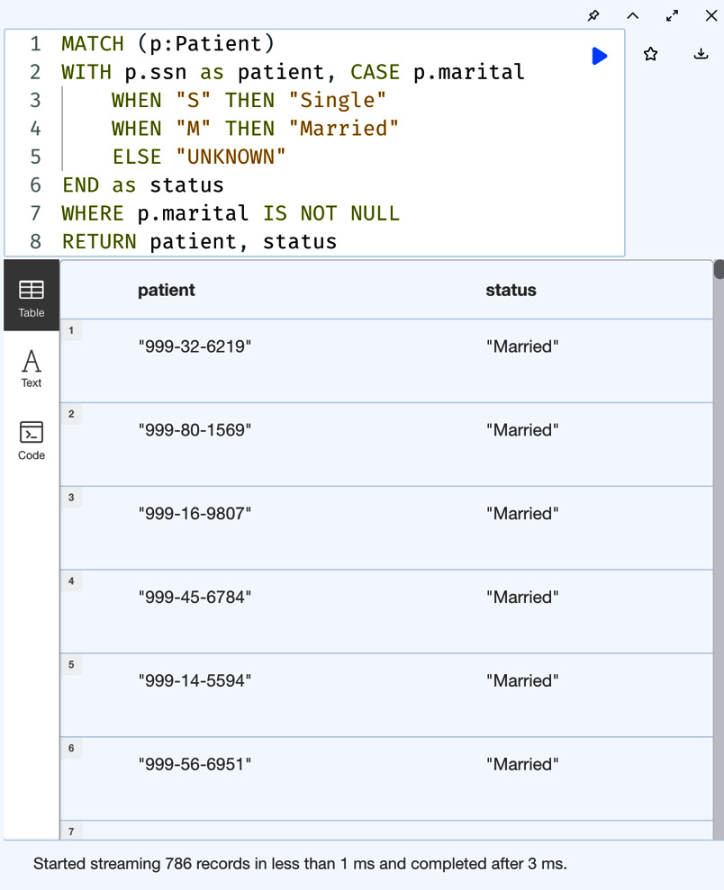
Figure 8.12 – Combining a simple CASE expression with a WITH clause

Also, we can see we are only getting 786 records returned from 1174 records, compared to the previous query we tried, as the WITH clause is eliminating all the patients who do not have a marital property value.

Working with generic CASE expressions

In generic CASE expressions, we do not have a default expression but each WHEN statement is a separate condition that is evaluated in order.

The syntax of a generic case expression looks as follows:

CASE
  WHEN predicate THEN result
  [WHEN …]
  [ELSE default]
END

We can see that we don’t have a value expression after the CASE clause here. Since there is nothing to evaluate here, the WHEN clause predicates take over.

We can describe each variable or argument in this syntax in the following way:

• predicate – This is the predicate or expression that is evaluated and then returns true or false. If this predicate returns true, then the corresponding result is returned.
• result – The expression whose output is returned when predicate is evaluated to true.
• default – The expression whose output is returned when all the predicates return false. Remember that since ELSE is optional, there is no need to have this expression. When this is missing, a null value is returned if all the predicates return false.

Let’s take a look at this:

WITH date().year as currentYear
MATCH (p:Patient)
RETURN p.ssn,
    CASE
        WHEN currentYear-p.birthDate.year < 16 THEN 'Child'
        WHEN 16 < currentYear-p.birthDate.year < 22 THEN 'Young Adult'
        WHEN 22 < currentYear-p.birthDate.year < 60 THEN 'Adult'
        WHEN 60 < currentYear-p.birthDate.year THEN 'Old'
    END as ageGroup

We can see in this query that we are taking the patients’ birth dates and categorizing them into age groups. While it is possible to build the same logic with a simple CASE expression, it would be very difficult and elaborate. We would need to have an individual WHEN clause for every value we could possibly have for the age value. A generic CASE expression can make it easier in this case.

As we can see from the following screenshot, we get the final value from the CASE expression returned as the age group value in the response.

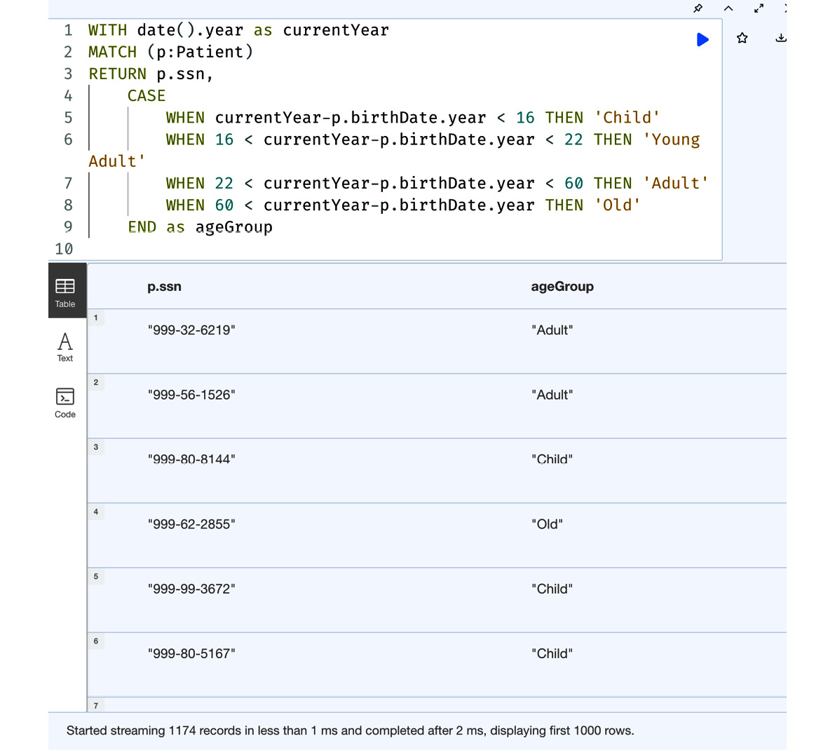
Figure 8.13 – A generic CASE expression usage

Another common use case for a generic CASE expression is to evaluate input data and then set the properties on the nodes dynamically. Since this is an expression, it can be used anywhere, as an expression is used to evaluate values.

Let’s look at how we can use a CASE expression to set the properties on a node. We can use the same expression we used in the previous query to create a new property on the patient node called ageGroup.

WITH date().year as currentYear
MATCH (p:Patient)
SET p.ageGroup =
    CASE
        WHEN currentYear-p.birthDate.year < 16 THEN 'Child'
        WHEN 16 < currentYear-p.birthDate.year < 22 THEN 'Young Adult'
        WHEN 22 < currentYear-p.birthDate.year < 60 THEN 'Adult'
        WHEN 60 < currentYear-p.birthDate.year THEN 'Old'
    END
RETURN p.ageGroup

In this query, we are reusing the CASE expression we used in an earlier query, setting the value created as a new property on the patient node, and then returning the final value.

As we can see from the following screenshot, we have set the ageGroup property on the patient node using the CASE expression value and the returned property value contains the new value.

Figure 8.14 – Using a generic CASE expression to set a property value on a node

We can see that a CASE expression can be a very powerful tool when manipulating data that makes sense either while writing data to a graph or when we are returning data.

We will explore the FOREACH clause next.

Working with the FOREACH clause

The FOREACH clause can be used to process a list and update the data in a graph. It can only be used to update data using the CREATE, MERGE, SET, DELETE, REMOVE, and FOREACH clauses. It is not possible to use the MATCH clause within FOREACH. Also, the variables in the context of the FOREACH clause are limited to its scope only and there is no option to remove those variables to be used after FOREACH.

Let’s look at an example usage:

MATCH (p:Patient)
WHERE p.marital IS NULL
WITH collect(p) as nodes
FOREACH( n in nodes | SET n:UNKNOWN_STATUS)

In this query, we are finding all the patients whose marital status is null, collecting all those patients into a list, and then using the FOREACH clause to add an UNKNOWN_STATUS label.

We can see from the screenshot that we have updated 388 patient nodes with the new label.

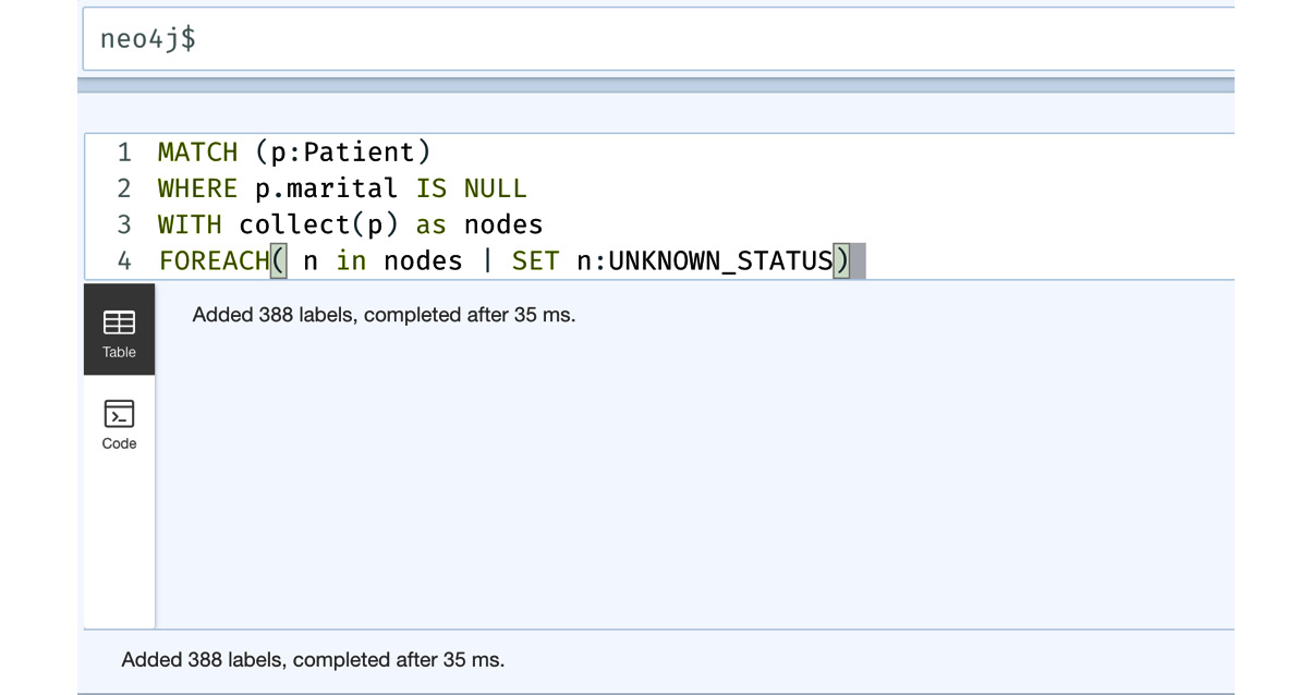
Figure 8.15 – Using FOREACH to add a new label to the node

Another usage of the FOREACH clause is to simulate an IF condition. Since there is no support for IF conditions in Cypher, we can leverage the way FOREACH works to simulate an IF condition.

Let’s build a query to get all the patient nodes and use the FOREACH clause to check for the new UNKNOWN_STATUS label and remove it. To achieve this, we need to leverage a CASE expression:

MATCH (p:Patient)
FOREACH(
    ignoreME in CASE WHEN p:UNKNOWN_STATUS THEN [1] ELSE [] END |
    REMOVE p:UNKNOWN_STATUS
)

In this query, we are leveraging FOREACH by preparing a list using the CASE expression first. The CASE expression applies the predicate. When it is true, it returns a list with one element, and when it is false, it returns an empty list. When a list with a single value is returned, the next set of statements is executed once. In this part, we are accessing the variable in the outer scope and removing the label on it.

From the following screenshot, we can see we have removed the label from exactly 388 nodes to whom we added this label in an earlier query.

x

Figure 8.16 – Using FOREACH to simulate an IF condition

FOREACH is a convenient way to process the lists to update the graph. But, when we need to do some extra work, such as finding other nodes before processing, this could be limiting. In that case, UNWIND is the best option to build the query.

With that in mind, now let’s explore the UNWIND clause.

Working with the UNWIND clause

We saw the usage of FOREACH in the previous section and explored how we can iterate a list and update the graph. But, its usage is limited. If we want to retrieve data from a graph based on the data in a list before we can update the graph, then it is not possible with FOREACH. The UNWIND clause allows us to be able to do this. Also, if we want to return some data while processing a list, then UNWIND is the option to do this.

Let’s take a look at the query we built to add a label in the previous section and build it using UNWIND:

MATCH (p:Patient)
WHERE p.marital IS NULL
WITH collect(p) as nodes
UNWIND nodes as n
SET n:UNKNOWN_STATUS

This does exactly what the FOREACH query did earlier. We find the patients who do not have a marital property set, and then we collect those nodes into a list and unwind that list to process one node at a time.

We can see from the screenshot that we updated 388 nodes, which is exactly what happened when we used FOREACH to process the list.

Figure 8.17 – Using UNWIND to process a list

When we want to process a list based on a condition, UNWIND provides good options. Let’s build a query using UNWIND to remove the label we added in the previous query:

MATCH (p:Patient)
WITH collect(p) as nodes
UNWIND nodes as n
WITH n
WHERE n:UNKNOWN_STATUS
REMOVE n:UNKNOWN_STATUS

We can see in this query that we have combined UNWIND and WITH to be able to process the data conditionally.

We can see from the following screenshot that we removed the label from exactly 388 nodes.

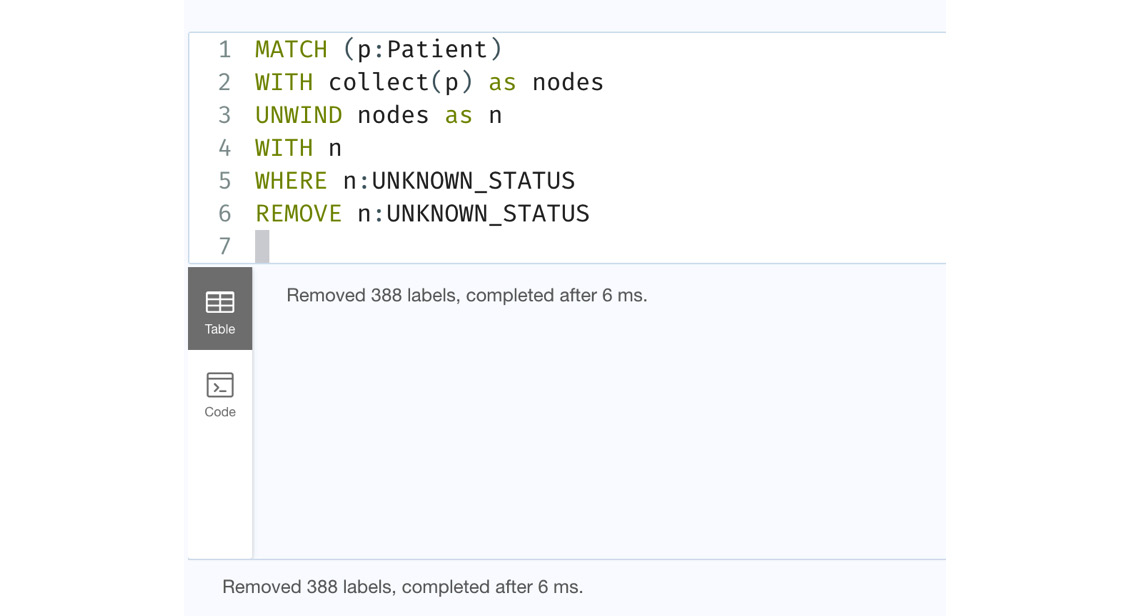
Figure 8.18 – Conditional processing data after UNWIND

From the last two sections, we can see that if we are doing some simple list processing and updating data, then FOREACH is the best and most simple option, as it isolates the processing. In this case, the UNWIND clause might be overkill, as it executes all the Cypher code below the UNWIND statement. If we want to elaborate data processing some more while iterating through the list and returning the data, then UNWIND is the best option.

We will take a look at using count stores next to build performant queries.

Working with count stores

Neo4j maintains certain data statistics as count stores. For example, there are node count stores that maintain the counts of nodes for each label type. Since our dataset is small, we will use PROFILE to understand how much work the database would be doing in terms of db hits, with and without count stores, for a given type of work. We will also take a look at how to leverage count stores to build more performant queries.

Let’s look at a sample node count store query:

PROFILE MATCH (n:Patient)
RETURN count(n)

This is a very basic query, and it leverages count stores instead of counting the nodes that have the Patient label.

We can see from the screenshot, the database uses NodeCountFromCountStore@neo4j, which looks for the totals from the count store. We can see that it takes one db hit. The performance is constant, no matter how large the database grows.

Figure 8.19 – A query using the node count store

We can see the performance gains when we are looking at traversals.

Let’s look at how most users try to build a query to count paths. We will take a look at the query that leverages the count stores to do the same work optimally.

Let’s look at the query first:

PROFILE MATCH p=(:Drug {code:'313820'})<--()
RETURN count(p)

In this query, we are searching for the drug node identified with the 313820 code and counting all the paths with incoming relationships to this node.

From the following screenshot, we can see that there are 115 incoming relationships to the node and it took 119 db hits to complete this query.

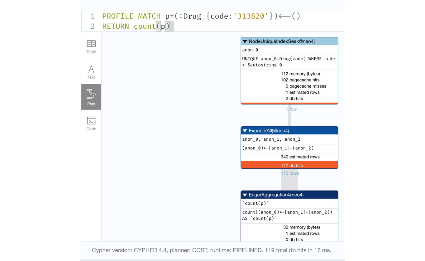
Figure 8.20 – Query to count incoming relationships to a node

Let’s rewrite this query using the size function:

PROFILE RETURN size((:Drug {code:'313820'})<--())

We can see this query is much simpler and leverages the expressive nature of Cypher combined with the size function to return the response.

We can see from the following screenshot that the performance of this query is exactly the same as the previous version.

Figure 8.21 – Using the size function to count the paths

Now, let us look at how to leverage the count stores to perform this operation more effectively:

PROFILE MATCH (d:Drug {code:'313820'})
RETURN size((d)<--())

We can see that we have changed our approach in this query. First, we wrote a query for the node and then we used the size function to find all the incoming relationships this node has.

From the screenshot, we can see it took only three db hits to perform the same activity to count the number of relationships.

Figure 8.22 – Optimal way to count the relationships

We are not using the count stores here as we are looking at data for a single node. If we look for incoming relationships for all the Drug nodes, it should leverage the count store.

Let’s try that:

PROFILE MATCH (:Drug)<-[r]-()
RETURN count(r)

This query returns the count of all incoming relationships of the Drug node.

We can see from the screenshot that it uses relationship count stores to return the data and it takes only one db hit.

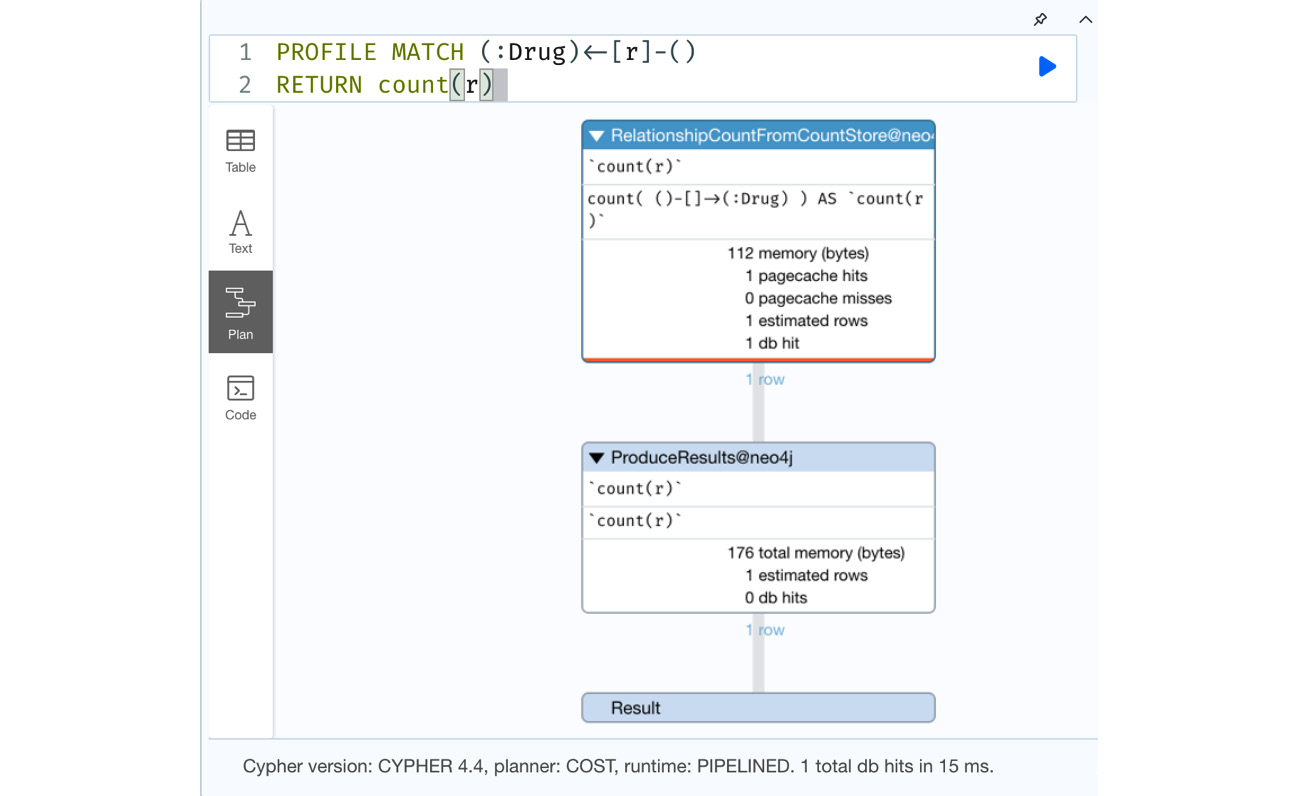
Figure 8.23 – Leveraging count stores to count relationships

There is a knowledgebase article (https://neo4j.com/developer/kb/fast-counts-using-the-count-store/) that talks about how to use count stores. This is updated with proper advice on how to leverage count stores and is kept updated with all the new releases.

We have looked at various aspects of Cypher used for building advanced queries. Let’s summarize what we have learned.

Summary

In this chapter, we explored using the WITH, CASE, FOREACH, and UNWIND clauses to build some advanced query patterns. We looked at chaining queries using the WITH clause to introduce new variables to the next part of the query, reducing the scope of the variables, and performing some conditional query executions. We looked at using a CASE expression to manipulate data to either write a graph or when returning a response. We looked at using the FOREACH and UNWIND clauses to iterate lists either to write a graph or to return data and discussed where graphs are appropriate to use and where not to use them. Finally, we looked at count stores, how we can leverage them in queries, and the optimal query patterns for counting the relationships of a single node.

In the next chapter, we will take a look at using the EXPLAIN and PROFILE keywords to identify query performance pain points and how to address them.