10

Using APOC Utilities

APOC is an acronym for Awesome Procedures On Cypher. It is an add-on library for Neo4j that provides a lot of procedures and functions that can extend Cypher to perform more complex operations. It’s built and maintained by Neo4j Labs. This chapter talks about using APOC utilities to extend the built-in capabilities of Cypher. It gives you more options to load CSV and JSON data, schedule timers, carry out ad hoc batch data modifications, and more.

We will cover these topics in this chapter:

• Installing APOC
• Working with data import and export
• Viewing database schema
• Executing dynamic Cypher
• Working with advanced path finding
• Connecting to other databases
• Using other useful methods

We will start with APOC plugin installation. We will take a look at the Neo4j Desktop plugin installation as well as installation on a server.

Installing APOC

APOC is a custom add-on library for Neo4j. We need to follow the appropriate installation process to make sure we can access all the capabilities provided by the APOC library. Since it uses core database APIs, we need to make sure we install the version of the library that matches the server version. If we do not follow these steps, the Neo4j server instance may not start:

1. First, we need to match the version of the library with the server we are running.

APOC releases use a consistent versioning scheme in the format <neo4j-version>.<apoc>. The trailing <apoc> version is incremented with each release.

The following table shows the compatibility of the APOC library with server versions. This table is partly taken from the APOC GitHub repository (https://github.com/neo4j-contrib/neo4j-apoc-procedures), which contains the full list:

Table 10.1 – APOC version to Neo4j version mapping

We will look at installing the plugin in Neo4j Desktop first.

2. When we click on the database in Neo4j Desktop, we can see the Plugins tab, as shown in the following screenshot:

Figure 10.1 – Neo4j Desktop – the Plugins tab

3. When you click the Plugins tab, it shows all the available plugins. To install the APOC plugin, click on APOC to show the option to install it. Click on the Install button to install the plugin. The advantage of Neo4j Desktop installation is that it updates the config file, neo4j.conf, automatically to enable all the features of APOC.

Next, we will take a quick look at how to install the plugin on the server.

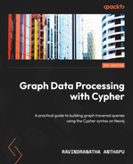
The following screenshot shows a tar install of the Neo4j server. We can see a list of directories that are part of the installation. The highlighted plugins directory is where we can install the plugins:

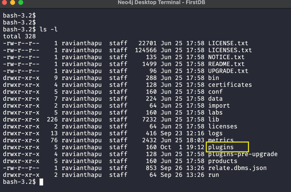
Figure 10.2 – Neo4j server installation directory

We can download the JAR file from the APOC releases at https://github.com/neo4j-contrib/neo4j-apoc-procedures/releases and copy it to the plugins directory. Once the JAR file is copied, we need to edit the neo4j.conf file found in the conf directory. For security reasons, all the procedures that use internal APIs are disabled by default. We can enable them by adding or updating the configuration:

dbms.security.procedures.unrestricted=apoc.*

The following screenshot shows the updated configuration highlighted. Once the configuration is changed, you need to restart the server for the changes to take effect:

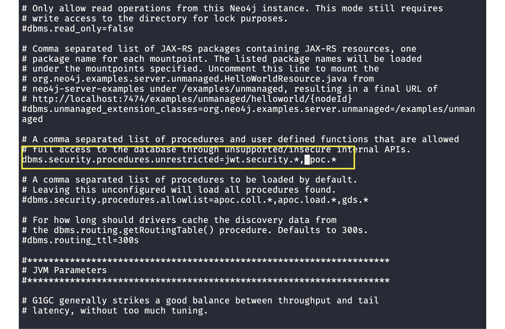
Figure 10.3 – Editing neo4j.conf to add the APOC configuration

Working with data import and export

APOC allows us to load data from various file formats, including CSV, JSON, Excel, XML, HTML, and GraphML. It can also export graph data as CSV or JSON. We will take a look at how to import data in each format.

First, we will take a look at importing CSV data.

Importing CSV data

We can use the apoc.load.csv method to load CSV data into a graph. It is very similar to the LOAD CSV command, but it provides a lot more options and is more tolerant of failures.

It provides these extra options when loading CSV files:

• It provides line numbers so that we can trace issues
• Both map and list representations for each CSV line are available
• The data is automatically converted to the correct data type and the data can be split into arrays as needed
• It is also possible to keep the original string-formatted values they are in the file
• There is an option to ignore fields, thus making it easier to assign a full line as properties
• It provides the ability to process headerless files
• It provides the ability to replace certain values with null
• You can also read compressed files

Note

Please note that if you are using Neo4j 5.0 or above database, the APOC library is split into Core, which is packaged with database and extended which user has to download manually and install. The method apoc.load.csv is moved to extended APOC library. Neo4j Desktop is not handling this aspect correctly. So to use this method you might have to manually download the plugin and copy it to plugins directory.

To load a CSV file from the local filesystem on the server, we need to follow these steps:

1. Let’s add this configuration first:

   Apoc.import.file.enabled=true
2. As shown in the following screenshot, click on … and select Settings… to update the configuration. It will bring up the settings screen:

Figure 10.4 – Selecting Settings… to update the configuration

3. As shown in the following screenshot, add the configuration and click on Apply to apply the changes. If the database has not started, then start the database. If it was already running, then it will be automatically restarted by Neo4j Desktop:

Figure 10.5 – Updating the configuration

Note

With this configuration enabled, you can only read the files from the import directory, as identified in the configuration.

4. Let’s create a sample test CSV file in the import directory with this content:

   id,firstName,lastName

   1,Tom,Hanks

   2,Meg,Ryan

Let’s look at an example.

The following statement loads a CSV file and returns the data as one row for each line. The returned data will have a line number, data as a list, and data as a map:

CALL apoc.load.csv("test.csv")

We can see in the screenshot that in each row, we have the line number of the CSV file, data as a list, and data as a map as well:

Figure 10.6 – apoc.load.csv sample usage

If we want to be able to load data from anywhere in the filesystem of the server, then we need to add this configuration:

1. First, let’s try without adding this configuration to understand how it behaves:

   apoc.import.file.use_neo4j_config=false

   In this case we are trying to load the file using the absolute path "/tmp/test.csv". CALL apoc.load.csv("/tmp/test.csv")
2. In the following screenshot, we can see that when we use the absolute path, it prepends the import directory location to it automatically and fails to load the file:

Figure 10.7 – Loading from an absolute path

Let’s update the configuration now:

3. Once we change the configuration and click on Apply button, the database will restart. Once it is restarted, we can try the command again:

Figure 10.8 – Adding the configuration to ignore neo4j_config for apoc

In the screenshot, we can see that we can load the file from /tmp/test.csv:

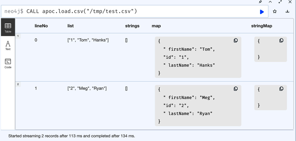
Figure 10.9 – Loading the CSV from an absolute path

Note

With neo4j configuration disabled, we can read any file in the whole file system that we have access to. This can be a security concern and should be done with the consultation of security team. Also, note that when you have this enabled, to read the files from neo4j import directory, you need to provide the full path. The previous command we tried to read the file from import directory will fail with this configuration added.

So far, we have only read a CSV file. Now let’s look at how to load it into a graph.

We will leverage the map output, as it has key/value pairs of the data:

CALL apoc.load.csv("/tmp/test.csv") YIELD lineNo, map
CREATE (p:Person {id:map.id, firstName: map.firstName, lastName: map.lastName})
RETURN lineNo

We can see from the query that we are taking the lineNo and map values returned by apoc.load.csv and using them to add data to a graph. As a response, we are returning the line numbers of the rows we have processed:

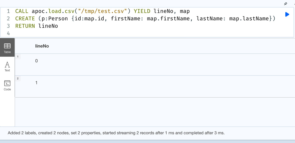
Figure 10.10 – Updating the data into a graph using apoc.load.csv

Note

One thing to note here is that this is a single transaction. If we have large amounts of data, then we must use apoc.periodic.iterate to process the data in batches. We will discuss this aspect later in the chapter.

Also, note that the directory names might be bit different for different operating systems. In windows the directory name could be "C:/temp" and in unix systems it could be "/tmp". Please verify the file system and update the URL appropriately.

We can also use URLs to load CSV data. We will take a look at loading JSON data next.

Importing JSON data

Loading JSON data is similar to loading CSV data. We can use the apoc.load.json method.

JSON data should look like this for this to work:

{ " firstName": "Tom", "id": "1", " lastName": "Hanks" }
{ " firstName": "Meg", "id": "2", " lastName": "Ryan" }

We can see each line is a JSON object. This format is mandatory if you want to use this method.

Let’s look at a simple example.

This reads the JSON file from /tmp/test.json and returns each line as a map. One thing that is different from reading CSV files is that we do not have the line number or a list representation of the data here. We will only have the map:

CALL apoc.load.json("/tmp/test.json")

We can see from the following screenshot that with this method, we only have a map representation of each line:

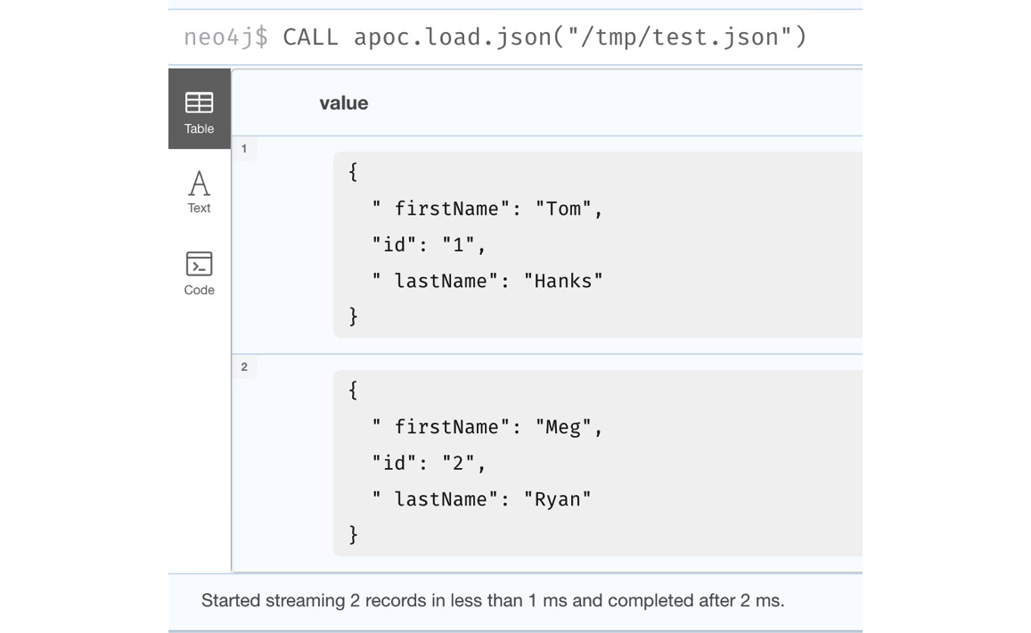
Figure 10.11 – Loading JSON

Let’s look at an example of loading JSON from a URL.

This code reads the JSON response from a URL and creates a map from it:

CALL apoc.load.json("https://api.stackexchange.com/2.2/questions?pagesize=5&order=desc&sort=creation&tagged=neo4j&site=stackoverflow&filter=!5-i6Zw8Y)4W7vpy91PMYsKM-k9yzEsSC1_Uxlf") YIELD value
UNWIND value.items AS i
RETURN i.title as title, i.owner as owner, keys(i) as keys
LIMIT 10

In the following screenshot, we can see the returned data. Also, we can see that some of the data can be nested JSON, and it is returned as a proper map instead of a string. This makes it easier to process nested JSON content easily:

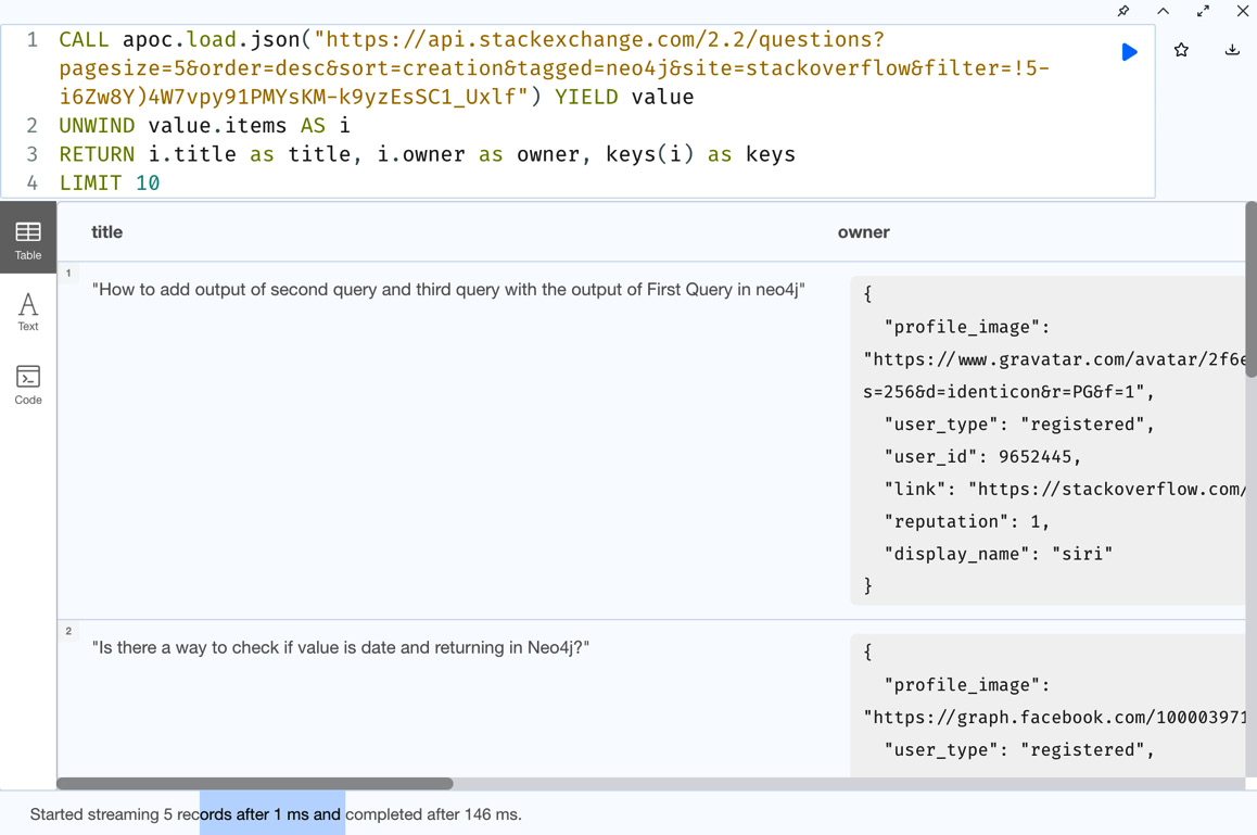
Figure 10.12 – Loading JSON with a URL

It’s also possible to use JSON PATH to limit what data we can try to process. The following table describes all the operators we can use to use JSON PATH expressions. The following table is from the APOC documentation (please see this link for the latest options https://neo4j.com/labs/apoc/4.1/import/load-json/):

Table 10.2 – JSON PATH expressions

Let’s look at an example of this.

The following query fields are identified by the owner key and return them from the JSON data:

CALL apoc.load.json("https://api.stackexchange.com/2.2/questions?pagesize=5&order=desc&sort=creation&tagged=neo4j&site=stackoverflow&filter=!5-i6Zw8Y)4W7vpy91PMYsKM-k9yzEsSC1_Uxlf", "$..owner") YIELD value
RETURN value
LIMIT 10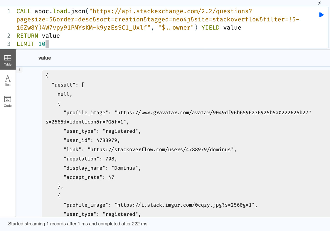

Figure 10.13 – Using JSON PATH to get fields at nested level

In the screenshot, we can see that we get a single JSON with a result field that represents the owner values for each entity. We can see that if there is no owner value in a given entity, we get a null value at that index. This pattern tries to find the values identified by a specific key at any depth. If we want to traverse the data exactly and get the values, we can try this approach.

This query traverses the JSON data with the exact path. First, it finds items values, which should be an array, and the owner value in each of those JSON values:

CALL apoc.load.json("https://api.stackexchange.com/2.2/questions?pagesize=5&order=desc&sort=creation&tagged=neo4j&site=stackoverflow&filter=!5-i6Zw8Y)4W7vpy91PMYsKM-k9yzEsSC1_Uxlf", "$.items[*].owner") YIELD value
RETURN value

We can see in the screenshot that the data returned is a bit different from the earlier query, even though we are requesting the data identified by the owner key. The first query tries to find the values at any depth for the specified key, and the second one traverses the exact path:

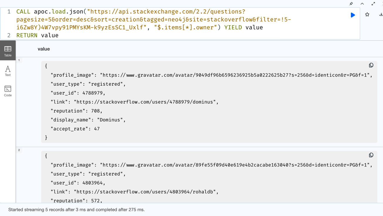
Figure 10.14 – JSON PATH with specific path traversal

There are scenarios when we want to load JSON from a URL and it requires authentication. In those cases, it might not be wise to have the credentials hardcoded in the query. We can use apoc.load.jsonParams to define the values in the apoc.conf file and have them referred in the Cypher.

Let’s look at the usage of this.

This configuration defines a value called mylink that can be retrieved with all the values in it as a map:

apoc.static.mylink.bearer=XXXX
apoc.static.mylink.url=https://test.mytest.com/data

This query will fetch the data from the URL specified in the configuration with an access token value, which also comes from the configuration and returns the data. If there is a payload that the URL requires, that can also be passed using this method:

WITH apoc.static.getAll("mylink") AS linkData
CALL apoc.load.jsonParams(
    linkData.url,
    {Authorization:"Bearer "+ linkData.bearer},
    null // payload
)
YIELD value
RETURN value

It is possible to load the data from other data formats, as mentioned earlier. We will not be discussing all these topics in this book, but you can read more at https://neo4j.com/labs/apoc/4.4/import/web-apis/.

We will now take a look at how we can see the database schema details using APOC.

Viewing database schema

Procedures with the apoc.meta suffix provide the functionality to inspect the metadata about graph, such as viewing the current schema or database statistics or inspecting the types. We will take a look at some important procedures:

The first one we will explore is the procedure to display the schema graph.

This displays the metadata graph that represents the schema of how nodes are related to each other:

CALL apoc.meta.graph()

In the following screenshot, we can see that the metadata graph seems very busy. This is because this representation does not understand nodes with multiple labels correctly and they are represented independently:

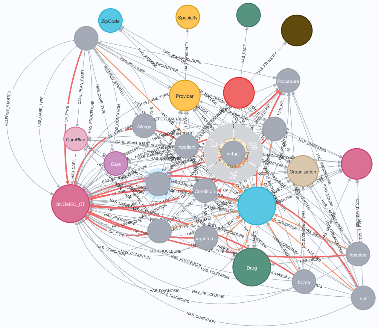
Figure 10.15 – Full APOC metadata graph

The nodes with the labels home, hospice, and so on are the secondary labels on the Encounter nodes.

We can have a cleaner representation using apoc.meta.subGraph. When we call this method, we can use, include, or exclude the node labels so that we can get the metadata graph the way we want with desired nodes and relationships.

The signature of this method is as follows:

apoc.meta.subGraph(config :: MAP?) :: (nodes :: LIST? OF NODE?, relationships :: LIST? OF RELATIONSHIP?)

The configuration options for this method are as follows:

• includeLabels: A list of the node labels to include in the graph. The default is to include all labels.
• includeRels: A list of the relationship types to include in the graph. The default is to include all relationship types.
• excludeLabels: A list of labels to exclude from the graph. The default is to not exclude any labels.
• Sample: The number of nodes to sample per label. The default is to scan 1000 nodes.
• maxRels: The number of relationships to be analyzed by the type of relationship and the start and end label. The default is 100 per type.

Let’s look at the usage of this method:

CALL apoc.meta.subGraph({
    excludeLabels:
        ['home', 'hospice',
        'virtual', 'wellness',
        'emergency', 'outpatient',
        'inpatient','urgentcare',
        'snf','ambulatory' ]})

In the query, we are only trying to exclude the node labels, as we know these are secondary labels. It is also possible to use include and not to exclude labels.

We can see in the screenshot that this graph is much cleaner than the other schema. This represents the actual database schema by removing the secondary nodes from the schema diagram:

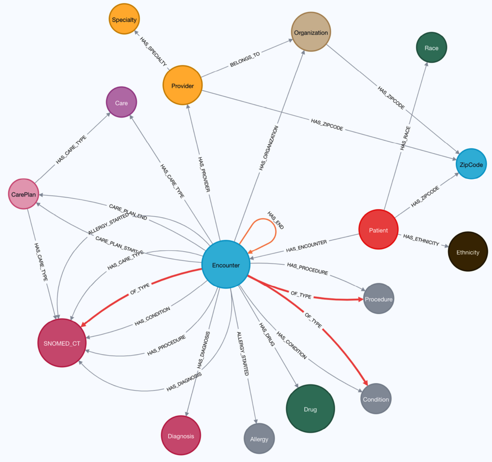
Figure 10.16 – Clean database schema

Now we will take a look at the apoc.meta.stats method to display the database statistics:

CALL apoc.meta.stats()

This will display database statistics such as the number of node labels, relationship types, and the number of nodes per label.

We can see in the following screenshot that this procedure displays the database statistics at a very granular level. It shows the number of nodes by label, the number of relationships by type, the number of relationships by start node label and relationship type, and so on:

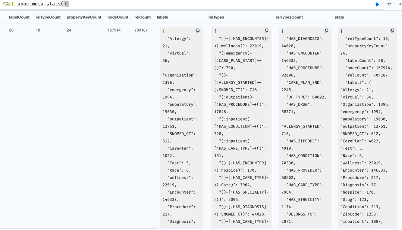
Figure 10.17 – Database statistics

This can be very useful for keeping track of now how the graph is growing by executing and keeping the results at regular intervals.

The next procedure, apoc.meta.data, provides property-level statistics. We can see from the name that it provides data-level statistics. The response is in tabular format; the previous procedure returns JSON:

CALL apoc.meta.data()

In the screenshot, we can see how the data is distributed at the property level. For each property, it shows at the node or relationship level how many times it is present in the graph:

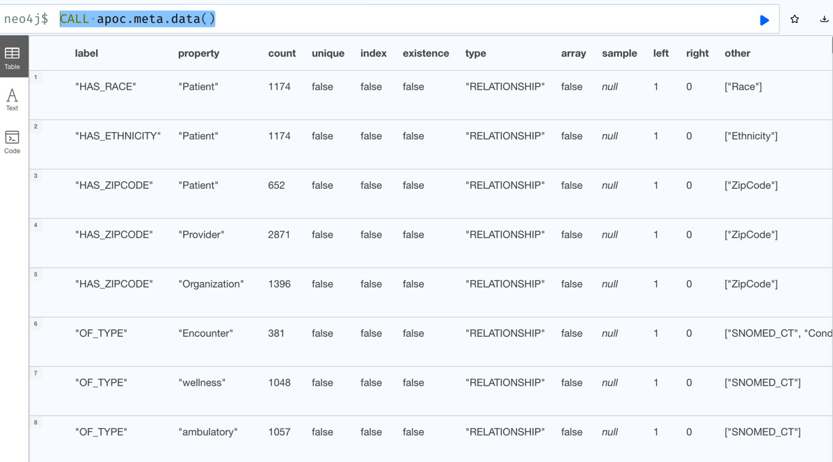
Figure 10.18 – Property-level statistics

If you would like to read more about these procedures and other schema-related procedures, visit https://neo4j.com/labs/apoc/4.4/database-introspection/meta/.

Next, we will take a look at how we can execute dynamic Cypher.

Executing dynamic Cypher

Cypher does not allow dynamic query execution. If you are getting a value in the data that you want to use as a label on the node, or you need to create a relationship with that name, that is not easy to do in Cypher. It is possible to use the FOREACH trick to check for the value and make the code deterministic, but this is not a practicable solution if the number of combinations is more than five, for example. In these scenarios, APOC procedures can help us to either to build a string and execute it or add or create nodes and relationships with dynamic values:

1. First, we will take a look at how to add a new label to a node using a dynamic value:

   WITH {label: "MyTest", id:10 , name: 'Another'} as data

   MERGE(p:Person {id:data.id})

   SET p.name=data.name

   WITH data, p

   CALL apoc.create.addLabels([p], [data.label])

   YIELD node

   RETURN node
2. This query creates a Person node with the data and appends the label from the input data using the apoc.create.addLabels method. You may have noticed here that we are preparing a list with a Person node and a new label because this method takes a list as its input parameter. The following screenshot shows that we have created the new node, and the node has the label from the data:

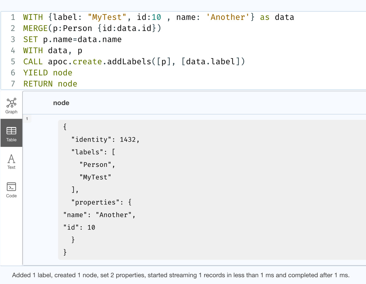
Figure 10.19 – Adding a label from the data

We needed to use the APOC method because if we try to add the label using a variable in Cypher, it will give a syntax error because Cypher does not support dynamic label addition. The following query shows a way to add a label dynamically, which will throw a syntax error:

WITH {label: "MyTest", id:10 , name: 'Another'} as data
MERGE(p:Person {id:data.id})
SET p.name=data.name, p:data.label

If we are getting all the labels from the data, then we can use the apoc.create.node or apoc.merge.node method to create the node as required. Let’s take a look at an example of this.

3. This query creates a node with labels "MyTest" and "Person" with an id value of 12, and we set the name to "Another":

   WITH {labels: ["MyTest", "Person"], id:12 , name: 'Another'} as data

   CALL apoc.merge.node(data.labels, {id:data.id}, {name:data.name}, null )

   YIELD node

   RETURN node

You can also create relationships dynamically using the apoc.create.relationship or apoc.merge.relationship method. You can read more about these methods at https://neo4j.com/labs/apoc/4.4/overview/apoc.merge/ and https://neo4j.com/labs/apoc/4.4/overview/apoc.create/.

When you need to execute a whole Cypher query as a string, then we can use apoc.cypher.doIt for write queries and apoc.cypher.run for read queries.

Let’s look at an example of this:

WITH {label: "MyTest", id:20 , name: 'Another'} as data
CALL apoc.cypher.doIt(
    "WITH $data as data MERGE(p:Person {id:data.id})
    SET p.name=data.name, p:" + data.label +
    " RETURN p",
    {data: data}
) YIELD value
RETURN value

This query does what we did before with the addLabels method, but we are building a dynamic Cypher query and executing it. In the screenshot, we can see that we are building a Cypher string from the data and executing it. This could be useful in a few scenarios where data is more dynamic:

Figure 10.19 – Dynamic Cypher query execution

We are not going to discuss all the available options for dynamic Cypher execution; you can read more about them at https://neo4j.com/labs/apoc/4.4/overview/apoc.cypher/.

Working with advanced path finding

Cypher provides means for variable pathfinding. But it has some limitations, as it is path distinct to make sure we don’t miss any paths. When there are loops in the graph, Cypher can be very memory intensive when we use variable-length paths. Also, if we need to change directions in the traversal or have node label filters, it is not possible in Cypher. This is where APOC provides an option with apoc.path.expandConfig that provides a lot of options with variable-length path expansion.

The syntax for this procedure looks like this:

apoc.path.expandConfig(
    startNode <id>|Node|list, ConfigMap
    ) YIELD path

The config map can have these values:

        minLevel
        maxLevel
        uniqueness
        relationshipFilter
        labelFilter
        uniqueness
        bfs:true,
        filterStartNode
        limit
        optional:false,
        endNodes
terminatorNodes
        sequence
        beginSequenceAtStart

All of these values are optional in the configuration, and we will take a look at how each of these values affects the path expansion. It starts from the start node or the list of nodes provided and traverses based on the configuration options provided. All the configuration options are optional. If you provide an empty configuration, then the equivalent Cypher query would look as follows:

MATCH path=(n)-[*]-() RETURN path

Let’s take a detailed look at the configuration options for this procedure:

• minLevel: The minimum path size to traverse. The default value is -1.
• maxLevel: The maximum path size to traverse. The default value is -1. The path expansion happens until all the other conditions are satisfied.
• relationshipFilter: The relationships to take into account when traversing the path. It can be one or more list of relationship types with optional directions separated by the | delimiter. Here are some examples:
  • CONNECTED>: Traverse only outgoing CONNECTED relationships.
  • <CONNECTED: Traverse only incoming CONNECTED relationships.
  • CONNECTED: Traverse the CONNECTED relationships irrespective of direction.
  • >: Traverse any outgoing relationship.
  • <: Traverse any incoming relationship.
  • CONNECTED>|<KNOWS: Traverse outgoing CONNECTED or incoming KNOWS relationships. This option is not possible with Cypher.
• labelFilter: A list of node labels separated by the | delimiter to include or exclude, or a termination of traversal or end node in the path. Let’s look at some examples:
  • -Test: Blacklisted label. This means this node should not exist in any of the paths that are returned. The default is that no label is blacklisted.
  • +Test: Whitelisted label. When we use this option, then all the node labels in the path should exist in the white label list. The default is that all labels are whitelisted.
  • >Test: End node in the path. Every path returned should have the end node label in this list. When we encounter an end label during traversal, we take that path and add it to the return list, but we continue traversing that path to see if there are other nodes with these labels to return a longer path. We can only traverse beyond the end node if the next node labels are whitelisted.
  • /Test: Terminate traversal once you encounter node labels in the termination list. We terminate our path expansion at the first occurrence of the labels in the termination list.
• Uniqueness:
  • RELATIONSHIP_PATH: This is the default and matches how Cypher works with variable-length paths. For each end node returned, there is a unique path from a start node, in this case in terms relationships traversed to reach the end node.
  • NODE_GLOBAL: A node cannot be traversed more than once in the whole graph.
  • NODE_LEVEL: All the node entities at the same level are guaranteed to be unique.
  • NODE_PATH: For each end node returned, there is a unique path from a start node, in this case in terms nodes traversed to reach the end node.
  • NODE_RECENT: This is very similar to NODE_GLOBAL, except for the fact that it only checks the last few recent nodes whose number can be specified by the configuration. This can be very useful when traversing large graphs.
  • RELATIONSHIP_GLOBAL: A relationship cannot be traversed more than once.
  • RELATIONSHIP_RECENT: This is very similar to NODE_RECENT but at the relationship level.
  • NONE: No restrictions in traversal, and results have to be managed by the user.
• Bfs: Use breadth-first search if true or depth-first if false. The default value is true.
• filterStartNode: This determines whether labelFilter and sequence apply to the start nodes. The default value is false.
• Limit: This determines how many paths are returned. The default value is -1, which means all paths should be returned.
• Optional: This determines whether the path expansion is like an optional match. If this is true, then a null value is returned if no paths are found, instead of there being no return value. The default is false.
• endNodes: A list of nodes that can be at the end of the path returned. This is optional as this information can also be provided in labelFilter. Providing those nodes here instead of in the labelFilter syntax could be more readable for users.
• terminatorNodes: A list of terminator nodes. Similar to the endNodes configuration option, this can be done using labelFilter.
• sequence: This tells the path expansion procedure the exact sequence of node labels and relationship types that have to appear in a sequence. Every path returned should start with this sequence and end with this sequence. When you use sequence, labelFilter and relationshipFilter are ignored.
• beginSequenceAtStart: This determines whether the sequence configuration should be applied to the start node or not.

Now let’s see a few examples of using this procedure. The PATIENT data model we have built may not benefit much from this procedure, so we will create some sample data and load it into a graph to see how this procedure can help us when traversing large graphs.

We can use this Cypher to create a test graph:

CREATE (:Test {id: 1})-[:CONNECTED]->(n1:Test {id: 2})
    -[:CONNECTED]->(n2:Test {id: 3})
    -[:CONNECTED]->(n3:Test {id: 4})
    -[:CONNECTED]->(n2)-[:CONNECTED]->(n5:Test {id: 6})
    -[:CONNECTED]->(n1),
    (n2)-[:CONNECTED]->(n7:Test {id: 8})
    <-[:CONNECTED]-(n3)-[:CONNECTED]->(n4:Test {id: 5})-[:CONNECTED]->(n1),
    (n7)-[:CONNECTED]->(n4)-[:CONNECTED]->(n5)
    -[:CONNECTED]->(:Test {id: 7})

The graph looks like this:

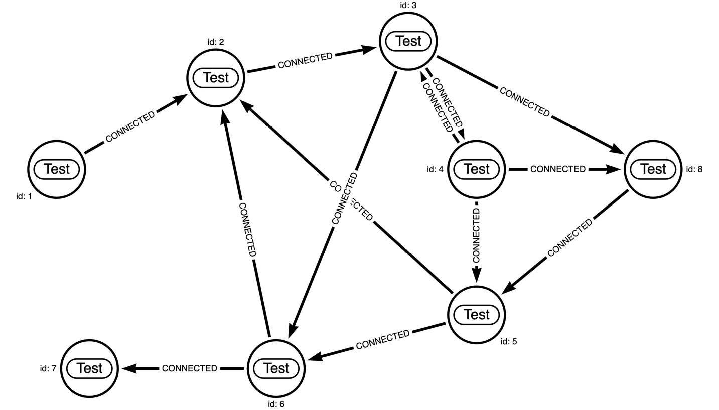
Figure 10.20 – Sample graph to test the APOC expandConfig procedure

This graph has a lot of loops. We will take a look at Cypher and APOC’s expand procedure to see how much work each query is doing, and how much data is returned:

• First, we will look at the Test node with id 1 and expand all the way. The Cypher looks like this:

  MATCH path=(:Test {id:1})-[:CONNECTED*]->()

  RETURN count(path)
• We are returning only the number of paths we have traversed instead of the actual graph. When browser displays the graph, it merges the duplicate data, meaning a node that appears in multiple paths will be shown only once:

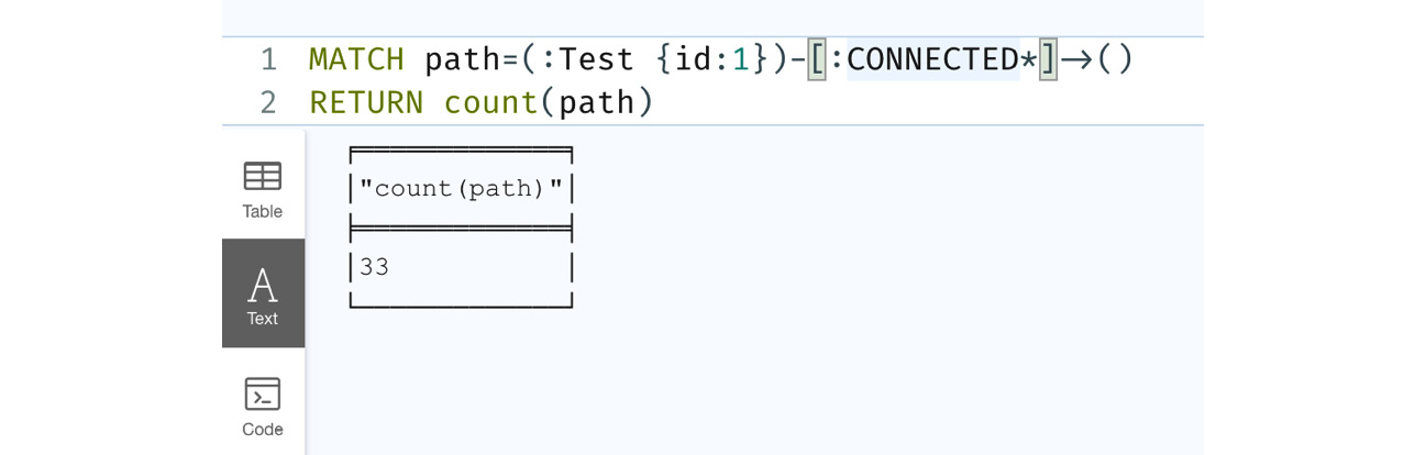
Figure 10.21 – Cypher variable length expansion

The screenshot shows that 33 paths are returned.

• Let’s look at the graph returned. We can see in the following screenshot that it is the complete test graph that we have created:

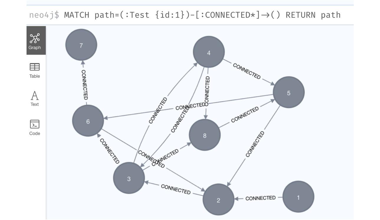
Figure 10.22 – Cypher variable length expansion graph

• Let’s look at the APOC expand procedure with the default configuration:

  MATCH (t:Test {id:1})

  WITH t

  CALL apoc.path.expandConfig(t,{relationshipFilter:"CONNECTED>"}) YIELD path

  RETURN count(path)

The original Cypher is much more readable and succinct than this query. Here, we have to get the node using MATCH first and then invoke the procedure.

• In the following screenshot, we can see that the number of paths is 34, which is one higher than previously, which is probably due to the start node being returned as a separate path:

Figure 10.23 – Variable expansion path with the default APOC expand configuration

Now, let’s look at using more configuration options and see how the procedure behaves.

We will take a look at the NODE_GLOBAL uniqueness option:

MATCH (t:Test {id:1})
WITH t
CALL apoc.path.expandConfig(
    t,
    {
        relationshipFilter:"CONNECTED>",
        uniqueness: "NODE_GLOBAL"
    }) YIELD path
RETURN count(path)

We have added NODE_GLOBAL to the configuration. Let’s look at the response.

In the following screenshot, we can see only eight paths being returned. Let’s see if the graph returned is the same:

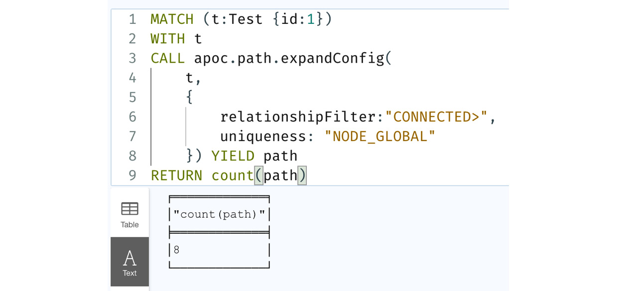
Figure 10.24 – Using the NODE_GLOBAL configuration

We can see from the graph that we have all the nodes but are missing the loop-back relationships here. This is because once we reach a node, we do not traverse those relationships. That’s why this graph is different from the other graph. If we are only interested in the nodes in the paths, then this option will not only be faster but use less memory as well:

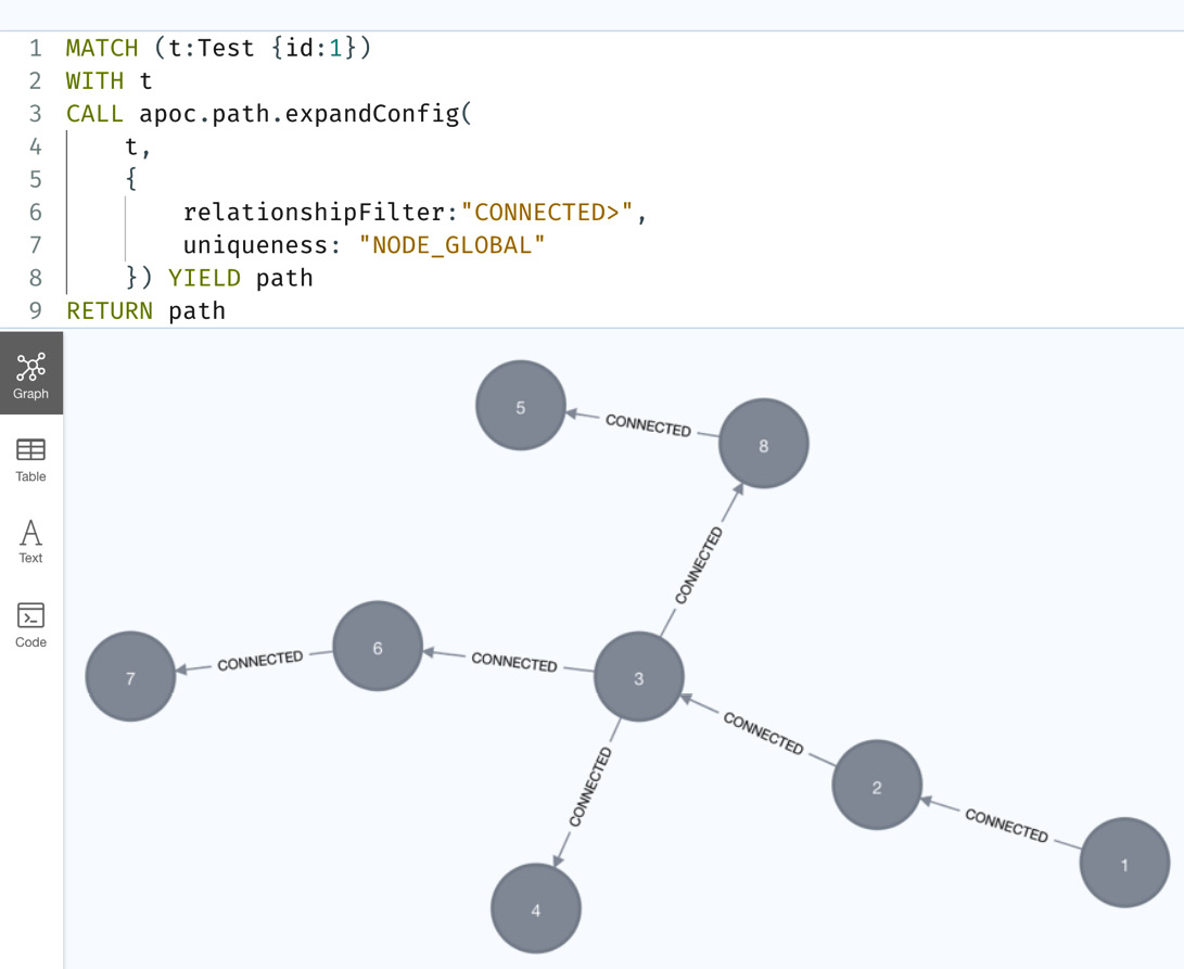
Figure 10.25 – Graph returned with the NODE_GLOBAL configuration

Let’s take a look at the RELATIONSHIP_GLOBAL configuration:

MATCH (t:Test {id:1})
WITH t
CALL apoc.path.expandConfig(
    t,
    {
        relationshipFilter:"CONNECTED>",
        uniqueness: "RELATIONSHIP_GLOBAL"
    }) YIELD path
RETURN count(path)

In this query, we are using RELATIONSHIP_GLOBAL as the configuration option.

Let’s look at the query response:

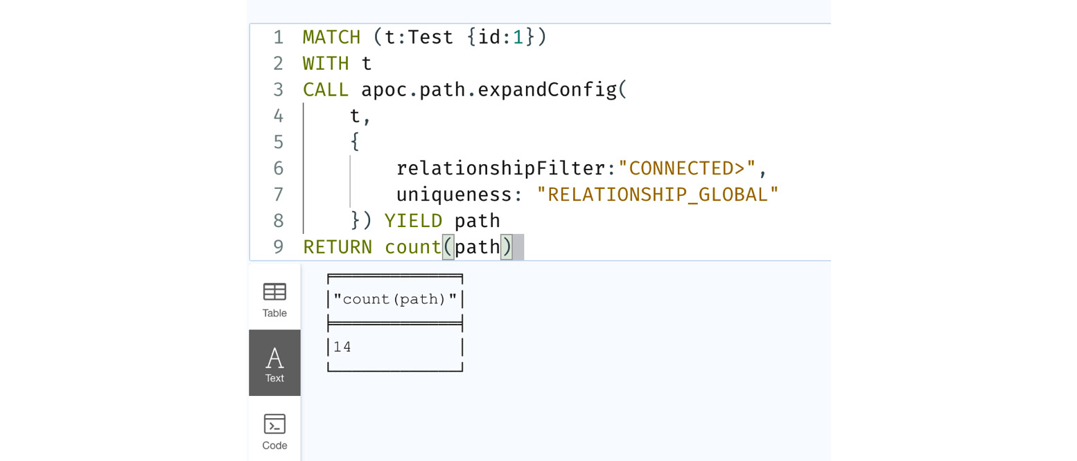
Figure 10.26 – Using the RELATIONSHIP_GLOBAL configuration

We can see in the following screenshot that we now have 14 paths returned. Let’s look at the graph being returned:

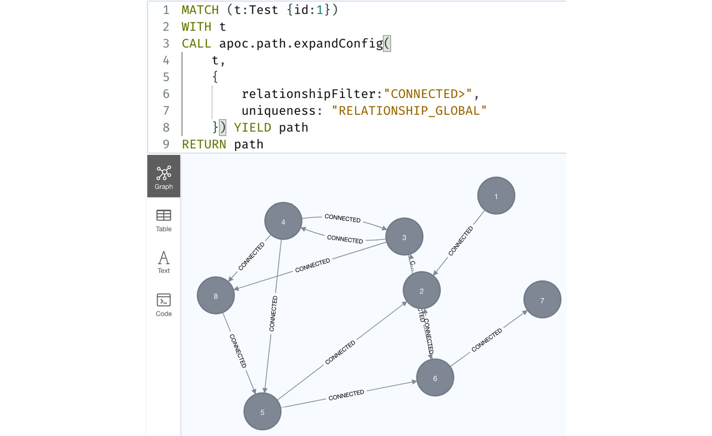
Figure 10.27 – Graph returned with the RELATIONSHIP_GLOBAL configuration

We can see the graph returned is the same in terms of nodes and relationships returned. In terms of graph visualization, this option can be faster and less memory intensive than the Cypher variable path expansion.

Let’s look at an example of termination node filter usage:

MATCH (t:Test {id:1})
WITH t
CALL apoc.path.expandConfig(t,
    { relationshipFilter:"CONNECTED>", labelFilter: "/Test"}) YIELD path
RETURN path

We are providing the termination nodes using the labelFilter option here.

In the screenshot, we can see that it is returning only one path because the first node it encountered was the Test node:

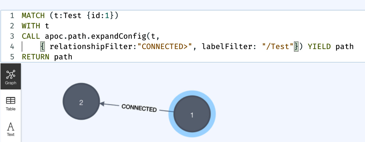
Figure 10.28 – Using the termination node filter

From the usage of the procedure, we can see that apoc.path.expandConfig is a very powerful way to traverse a graph using various conditional traversals and can be a very good utility to be aware of when we are writing complex Cypher queries.

APOC also provides utility procedures to enable you to connect to other databases. We will take a look at those procedures in the next section.

Connecting to other databases

APOC provides ways to integrate with various databases to read or modify data. We will take a look at each of these methods to see how we can interact with other databases from Cypher:

• JDBC: To connect to JDBC-compliant data using a JDBC driver, we need to make sure to add the required JARs to the plugins directory. Once you have added the JARs to the plugins directory, restart the server instance.

To make sure the jdbc driver is loaded, we need to execute the load driver method first as shown here:

CALL apoc.load.driver("com.mysql.test.Driver")

Once the driver is loaded, we can query the data using the load.jdbc method. We will take a look at an example query here:

WITH "jdbc:mysql://localhost:3306/mydb?user=root" as url
CALL apoc.load.jdbc(url,"person") YIELD row
RETURN row

This query returns each row as a map from the person table in the mydb database. You can take this row and add it to a graph or do other work.

• Elasticsearch: APOC provides a lot of functions to interact with Elasticsearch to read, write, and query. Similar to JDBC drivers, you need to copy the required JAR files to the plugins directory. Some of the methods available are as follows:
  • apoc.es.get: This retrieves documents from the specified server and index.
  • apoc.es.query: This method executes the specified query against the provided server.
  • apoc.es.post: This performs the POST function against the specified server.
  • apoc.es.put: This performs the PUT action against the specified server.

You can read more about these methods and examples at https://neo4j.com/labs/apoc/4.4/database-integration/elasticsearch/.

• MongoDB: Similar to the other database integration, you would need to copy the required JAR files to the plugins directory. Some of the methods provided are as follows:
  • apoc.mongodb.find: Finds documents of a given type
  • apoc.mongodb.insert: Inserts the specified document into MongoDB
  • apoc.mongodb.update: Updates the specified document
  • apoc.mongodb.delete: Deletes the specified document

You can read more about these methods and examples at https://neo4j.com/labs/apoc/4.4/database-integration/mongodb/.

We talked about a few of the database integrations available in APOC. For a full list of functionality and documentation, please visit https://neo4j.com/labs/apoc/4.4/database-integration/. A complete discussion on the usage with examples is beyond the scope of this book.

Note

While it is convenient for these functions to talk to other databases from Cypher, you need to keep in mind that they are running on Neo4j server instances and using the heap on the server. The quality of those queries can have a negative impact on graph database performance. In some scenarios, these queries can even crash the server.

We will take a look at some other useful procedures next.

Using other useful methods

There are a few other procedures that are useful when we are manipulating graphs. One of the most widely used procedures in this regard is apoc.periodic.iterate. Before the CALL subquery capability was added to Cypher, this was the only way to manipulate a graph in a batch manner.

Please note that this syntax is provided by the APOC documentation (https://neo4j.com/labs/apoc/4.4/overview/apoc.periodic/apoc.periodic.iterate/). You can visit that link for the latest syntax. The syntax of this procedure looks like this:

apoc.periodic.iterate(cypherIterate :: STRING?, cypherAction :: STRING?, config :: MAP?) :: (batches :: INTEGER?, total :: INTEGER?, timeTaken :: INTEGER?, committedOperations :: INTEGER?, failedOperations :: INTEGER?, failedBatches :: INTEGER?, retries :: INTEGER?, errorMessages :: MAP?, batch :: MAP?, operations :: MAP?, wasTerminated :: BOOLEAN?, failedParams :: MAP?, updateStatistics :: MAP?)

This procedure takes two Cypher strings and a configuration as parameters. The first Cypher statement is called the data statement. We execute this query, and the returned data is passed to the second action statement. The action statement is executed with data collected in batches from the first statement.

Let’s look at an example. The following query shows a simple query that adds a new label to a node in a batch manner:

 CALL apoc.periodic.iterate(
    "MATCH (person:Person) WHERE (person)-[:ACTED]->() RETURN person ",
    "SET person:Actor",
    {batchSize:100, parallel:true})

We can see the data query, action query, and configuration details here.

The data query returns all the people who have an ACTED relationship. In the action query, we are adding an extra label, Actor, to it. It collects 100 people at a time (the batch size) and executes the second action query with that batch. If we have 1,000 people, then the action query is executed 10 times, with 100 people per batch.

Another thing we should mention here is that we are using the parallel: true option in the configuration. This means that the action query can be run in parallel.

This is the most common usage of this procedure. While the CALL subquery can still be used, most of this it is not possible to execute the action queries in parallel in subqueries.

Note

When you are using the parallel: true option, you need to be aware of locking.

If you are creating relationships or deleting them, parallel: true can be troublesome depending on how you get the data from the data query.

When adding/updating/deleting properties or labels, parallel: true can be safe.

Another useful procedure is apoc.do.when. We know Cypher does not have an IF/ELSE construct. This procedure fills in that gap. The syntax of this procedure is as follows:

apoc.do.when(
    condition :: BOOLEAN?,
    ifQuery :: STRING?,
    elseQuery =  :: STRING?,
    params = {} :: MAP?) :: (value :: MAP?)

We can see that this works pretty similarly to an IF – THEN – ELSE construct. We can simulate an IF condition using a FOREACH clause in Cypher. But one disadvantage is that we cannot do a MATCH inside a FOREACH clause or invoke other procedures. Even the nodes or relationships created or updated in a FOREACH clause are not visible outside of it. This procedure removes these obstacles. We can perform any Cypher query and provide the response to be processed in the next steps.

Let’s summarize our understanding of APOC procedures.

Summary

We have looked at installing the APOC plugin, using various APOC procedures to review the database schema and statistics, loading data into graphs using CSV or JSON files, executing dynamic Cypher statements, traversing graphs using path expansion with various configuration options, and connecting to other databases from Cypher. We have also reviewed a few important procedures that we can use to build complex queries easily. What we have covered in this chapter are only a few representative procedures. To take a look at what other procedures and functions are available, along with examples, please visit https://neo4j.com/labs/apoc/4.4/. There, you can find extensive documentation about all the functionality provided, along with detailed examples.

In the next chapter, we will take a look at the ecosystem surrounding Cypher.