3

Loading Data with Cypher

To load data into a graph, we need to understand how to map the source data to a graph model. In this chapter, we will discuss mapping the source data to a graph model, what decisions drive the graph model, and how to load the data into this model. In the last chapter, we looked at Cypher syntax and what queries can be used to create, update, or delete nodes, relationships, and properties. We will use these patterns to map the CSV files to a graph model as we go through each file and build Cypher queries to load this data in a transactional manner.

Neo4j is an ACID-compliant database. To load data into Neo4j, we would need to leverage transactions similar to those in an RDBMS, and Cypher is the query language we use to load the data. There are multiple options to load data into Neo4j using Cypher. They are LOAD CSV, using Neo4j client drivers, and using apoc utilities.

In this chapter, we will cover these topics:

• Before loading the data
• Graph data modeling
• Loading data with LOAD CSV
• Loading data with LOAD CSV using batching
• Loading data using client drivers
• Mapping the source data to graph

We will first take a look at the options available to load the data using Cypher. Once we understand how to load the data, we will look at graph data modeling and take a step-by-step approach to reviewing the data and how the model evolves as we keep adding data to the graph.

Before loading the data

To start loading data with Cypher, we need to build the graph data model first. While Neo4j is a schemaless database, we still need to understand how our data will look in a graph representation and whether it can answer our questions effectively. This process involves understanding the data and seeing what the nodes and relationships would be and what would map to the properties. For example, say we have a list of events with date values in the source data:

• If we are looking for events in the sequence they occurred, then we can have the date as a property on the event node
• If our requirements are to look at the set of events by date, then making the date a node would help us to answer those questions more effectively

We will discuss these aspects in more detail with a sample dataset later in this chapter.

We will introduce the basics of graph data modeling first and the tools available for it before we continue with the data loading discussion.

Graph data modeling

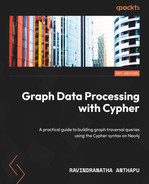
To build a data model, you can use the Arrows.app site (https://arrows.app). The following screenshot shows an example diagram:

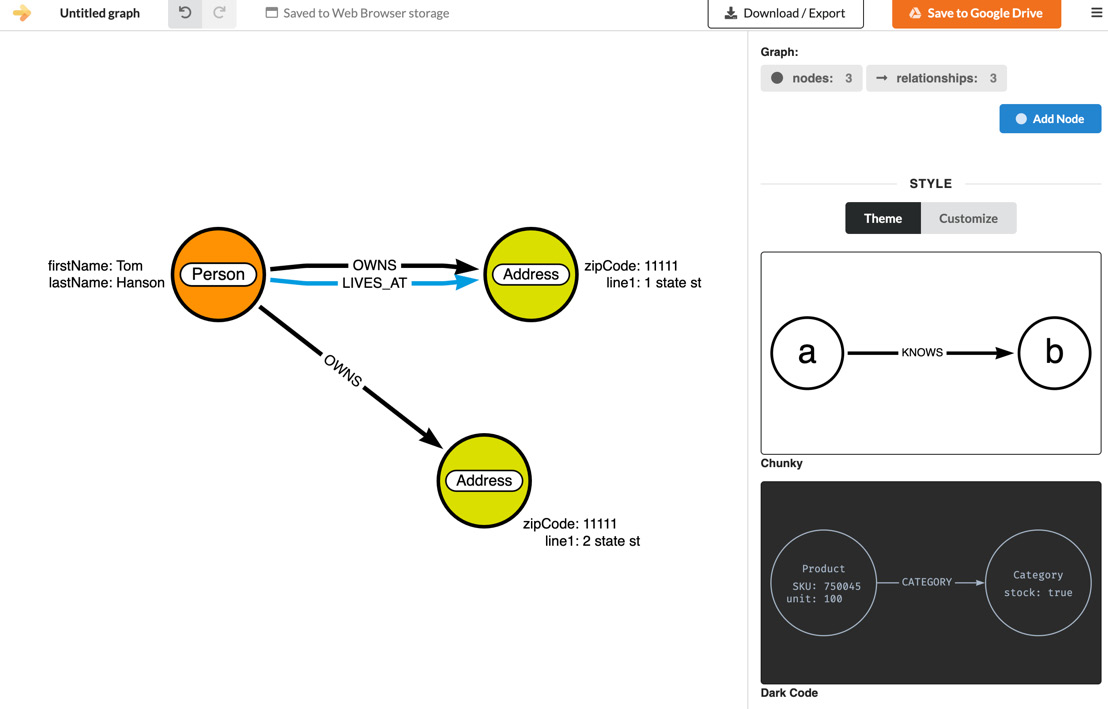
Figure 3.1 – Graph data model

This can be thought of as a data diagram where a set of data is drawn as a graph. It is possible to directly load the data into Neo4j with an assumed data model by skipping this part, but this approach can facilitate larger team collaboration and arrive at a better graph model. One of the aspects of this approach is to represent part of the data as a graph diagram and see how the graph traversal would work to answer our questions.

Say we have a set of questions; we can try to trace the model to see whether we can answer them:

• How many addresses are OWNED by a person?
  • Find the person, traverse the OWNS relationship, and count the addresses
• At which address is a person living?
  • Find the person and traverse the LIVES_AT relationship to find the required address
• How many addresses has the person lived at?
  • We cannot answer this question with this model, as we only know the current address the person lives at. If this is a question that needs to be answered, then we need to update the graph data model.

We will review the options available to load the data into the database first and then continue to loading data for a sample application.

Loading data with LOAD CSV

LOAD CSV can be used to load the data from the following:

• Local filesystem on a server: The files have to be in the import directory of the server. LOAD CSV cannot access random locations.
• From a URL: It is possible to load the data from any URL that is accessible from the server.

Note

Remember that LOAD CSV is the command issued by the client to the server. If it is a URL, it should be accessible from the server, as the server will try to download the CSV content from the URL and process the next steps.

We will take a look at some LOAD CSV usage examples in this section.

When the server processes the CSV file, each row is converted into a MAP or LIST type depending on how the command is issued.

LOAD CSV without headers

When we use the LOAD CSV command without a header option, then each row is mapped as a list. The screenshot here shows how this would look:

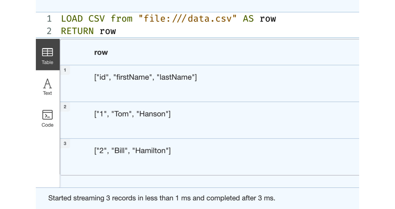
Figure 3.2 – LOAD CSV from the browser

From the picture, we can see the three rows of data. We can also observe that the header is also returned as a row since we did not tell the LOAD CSV command to read with headers.

LOAD CSV with headers

When we use the LOAD CSV command with the header option, then each row of the data gets mapped into a map object (key-value pairs) with each header column being the key and the corresponding value in the row being the value. The screenshot here shows how this would look:

Figure 3.3 – LOAD CSV WITH HEADERS from the browser

We can see here that the data is returned as a map. The server reads the header row and uses the values there as keys for values. This is the most common usage of the LOAD CSV command.

Caution

The LOAD CSV command is executed as part of a single transaction. When you are processing a large dataset or have a small heap, then you should process the data in batches. Otherwise, it could crash the server with an out of memory exception, if no memory guard is set up. If the server has a memory guard, then the query will fail.

Loading data with LOAD CSV using batching

When you have a large amount of data, then you should try to commit the data in batches so that you do not need a large heap to process the data.

There are two options to process the data in batches.

• USING PERIODIC COMMIT
• CALL IN TRANSACTIONS

Let’s now go through these two options next.

USING PERIODIC COMMIT

This is an older syntax and is deprecated from Neo4j 4.4 version onward, but if you are using Neo4j software prior to this version, then you must use this option to commit data in batches:

:auto USING PERIODIC COMMIT 1
LOAD CSV WITH HEADERS from "file:///data.csv" AS row
WITH row
MERGE (p:Person {id:row.id})
SET p.firstName = row.firstName,
    p.lastName = row.lastName

This command will execute a commit after processing one row at a time.

CALL IN TRANSACTIONS

This is the newer syntax and is available from Neo4j 4.4 onward:

:auto LOAD CSV WITH HEADERS from "file:///data.csv" AS row
CALL {
    WITH row
    MERGE (p:Person {id:row.id})
    SET p.firstName = row.firstName,
        p.lastName = row.lastName
} IN TRANSACTIONS OF 1 ROWS

This command will execute the commit after processing one row at a time.

Loading data using client drivers

When you use LOAD CSV, the server is responsible for downloading the CSV content and executing the Cypher statements to load the data. There is another option to load the data into Neo4j. We can use Neo4j drivers from an application to load the data.

Neo4j documentation - Drivers and APIs (https://neo4j.com/docs/drivers-apis/) contains the documentation on all the options available. In this section, we will discuss using Java and Python drivers to load the data.

Neo4j client applications make use of a driver that, from a data access perspective, will work as the main form of communication within a database. It is through this driver instance that Cypher query execution is carried out. An application should create a driver instance and use it in the application. The driver communicates with the Neo4j server using the Bolt protocol.

Let’s take a look at how we can create a driver instance here:

• This shows how a driver instance can be created in Java:

  import org.neo4j.driver.AuthTokens;

  import org.neo4j.driver.Driver;

  import org.neo4j.driver.GraphDatabase;

  public class DriverLifecycleExample implements

  AutoCloseable {

      private final Driver;

      public DriverLifecycleExample(

        String uri, String user, String password) {

                   driver = GraphDatabase.driver(

                   uri, AuthTokens.basic(

                         user, password));

              }

       @Override

       public void close() throws Exception {

             driver.close();

       }

  }
• This shows how a driver instance can be created in JavaScript applications:

  const driver = neo4j.driver(uri, neo4j.auth.basic(

       user, password))

  try {

        await driver.verifyConnectivity()

       console.log('Driver created')

  } catch (error) {

       console.log(`connectivity verification failed.

       ${error}`)

  }

  // ... on application exit:

  await driver.close()
• This shows how a driver instance can be created in a Python application:

  from neo4j import GraphDatabase

  class DriverLifecycleExample:

      def __init__(self, uri, auth):

             self.driver = GraphDatabase.driver(

                   uri, auth=auth)

      def close(self):

  self.driver.close()

From the code examples, we can see that to create a driver instance, we need the URL for the Neo4j server instance and credentials. The URL should use one of the URI schemes given as follows:

Figure 3.4 – URI schemes available

We will take a look at what each of these URI schemes means and how it works next.

URI schemes

This section describes how each URI scheme works and differs from the others and how to choose one to connect to a Neo4j instance.

• neo4j: This is the default URI scheme used by Neo4j from 4.0 onward. When you use this scheme in the URL, then the driver can connect to a single Neo4j instance or a cluster. This scheme is cluster aware. When this scheme is used, the communication with the server is not encrypted.
• neo4j+s: This scheme works exactly how the neo4j scheme works with the exception that all the communication with the server is encrypted.
• neo4j+ssc: This scheme works exactly how the neo4j scheme works with the exception that all the communication with the server is encrypted, but the certificate chain validation is skipped, which is mandatory in the neo4j+s scheme. You will use this option when the neo4j server is configured with a self-signed certificate for encryption purposes.
• bolt: When you use this scheme in the URL, then the driver can only connect to a single neo4j instance. This scheme is not cluster aware. In a cluster environment, if you use this scheme to connect to a FOLLOWER node, then performing write queries will fail.
• bolt+s: This scheme works exactly how the bolt scheme works with the exception that all the communication with the server is encrypted.
• bolt+ssc: This scheme works exactly how the bolt scheme works with the exception that all the communication with the server is encrypted, but the certificate chain validation is skipped, which is mandatory in the neo4j+s scheme. You will use this option when the neo4j server is configured with a self-signed certificate for encryption purposes.

Let’s move on to a Neo4j session next.

Neo4j sessions

Once the driver is created to execute the queries you need to create a neo4j session, which provides these options to execute queries:

• run: This is the basic method to execute the queries with or without parameters. This is a WRITE transaction, so in the cluster, all the queries will go to the LEADER instance.
• readTransaction: When you execute a readTransaction method in a clustered environment, the driver will find a FOLLOWER or READ REPLICA instance for the database and will execute the query on that instance. On a single node, there is no change in behavior. When you are building a client application, you should make sure you use this method for read queries. When you use this function, the transaction will be retried automatically when a transaction is cancelled or rolled back with exponential backoff.
• writeTransaction: When you execute a readTransaction method in a clustered environment, the driver will find the LEADER instance for the database and will execute the query on that instance. On a single node, there is no change in behavior. When you are building a client application, you should make sure you use this method for read queries. When you use this function, the transaction will be retried automatically when a transaction is canceled or rolled back with exponential backoff.

Let’s take a look at the code examples for each of these methods. We will take a look at the run method usage.

1. First, we will take a look at a Java code snippet:

   public void addPerson(String name) {

       try (Session = driver.session()) {

           session.run("CREATE (a:Person {name: $name})",              parameters("name", name));

       }

   }
2. Now let’s look at a Python code snippet:

   def add_person(self, name):

       with self.driver.session() as session:

           session.run("CREATE (a:Person {name: $name})",              name=name)
3. Finally, let’s take a look at the JavaScript usage of this method:

   const session = driver.session()

   const result = session.run('MATCH (a:Person) RETURN a.name ORDER BY a.name')

    const collectedNames = []

   result.subscribe({

     onNext: record => {

       const name = record.get(0)

       collectedNames.push(name)

     },

     onCompleted: () => {

       session.close().then(() => {

         console.log('Names: ' + collectedNames.join(', '))

       })

     },

     onError: error => {

       console.log(error)

     }

   })

We will take a look at the writeTransaction usage now:

1. This is the Java code example for this method:

   public void addPerson(final String name) {

        try (Session = driver.session()) {

              session.writeTransaction(tx -> {

                    tx.run("CREATE (

                          a:Person {name: $name})",

                          parameters("name", name)

                          ).consume();

                    return 1;

              });

        }

   }
2. Now, here’s a Python example of this function usage:

   def create_person(tx, name):

        return tx.run("CREATE (

              a:Person {name: $name}) 

        RETURN id(a)", name=name).single().value()

   def add_person(driver, name):

        with driver.session() as session:

              return session.write_transaction(

                   create_person, name)
3. Finally, here’s a JavaScript usage of this function:

     const relationshipsCreated = await session.writeTransaction(tx =>

       Promise.all(

         names.map(name =>

           tx

             .run(

               'MATCH (e:Person {name: $p_name}) ' +

                 'MERGE (c:Company {name: $c_name}) ' +

                 'MERGE (e)-[:WORKS_FOR]->(c)',

               { p_name: name, c_name: companyName }

             )

             .then(

               result =>

             result.summary.counters.updates()

               .relationshipsCreated)

             .then(relationshipsCreated =>

               neo4j.int(relationshipsCreated).toInt()

             )

         )

       ).then(values => values.reduce((a, b) => a + b))

     )

     console.log(`Created ${relationshipsCreated} employees relationship`)

   } finally {

     await session.close()

   }

We will take a look at readTransaction function usage now:

1. This is the Java usage of this function:

   public List<String> getPeople() {

       try (Session = driver.session()) {

           return session.readTransaction(tx -> {

               List<String> names = new ArrayList<>();

               Result = tx.run(

   "MATCH (a:Person) RETURN a.name ORDER BY a.name");

               while (result.hasNext()) {

                   names.add(result.next().get(0).asString());

               }

               return names;

           });

       }

   }

The following code segment is the Python usage of the same function:

def match_person_nodes(tx):
    result = tx.run("MATCH (a:Person) RETURN a.name ORDER BY a.name")
    return [record["a.name"] for record in result]
with driver.session() as session:
    people = session.read_transaction(match_person_nodes)

2. Finally, here’s the JavaScript usage of the same function:

   const session = driver.session()

   try {

     const names = await session.readTransaction(async tx => {

       const result = await tx.run('MATCH (a:Person) RETURN a.name AS name')

       return result.records.map(record => record.get('name'))

     })

Now that we have seen the client aspects, we will take a look at a sample dataset and review the steps to load the data into a graph.

Mapping the source data to graph

When we want to load the data into a graph using Cypher, we need to first map the data to the graph. When we first start mapping the data to the graph, it need not be the final data model. As we understand more and more about the data context and questions, we want to ensure the graph data model can evolve along with it.

In this section, we will work with the Synthea synthetic patient dataset. This site, Synthea – Synthetic Patient Generation (synthetichealth.github.io/synthea), provides the outlay of it. This website describes Synthea data like this:

“Synthea™ is an open-source, synthetic patient generator that models the medical history of synthetic patients. Our mission is to provide high-quality, synthetic, realistic but not real, patient data and associated health records covering every aspect of healthcare. The resulting data is free from cost, privacy, and security restrictions, enabling research with Health IT data that is otherwise legally or practically unavailable.”

This was built by the MITRE corporation to assist researchers.

A Synthea record (https://github.com/synthetichealth/synthea/wiki/Records) describes the data generated by Synthea. It can generate data in FHIR, JSON, or CSV format. In FHIR and JSON format, a file for each patient is generated. In CSV format, it generates one file per functionality.

After running Synthea, the CSV exporter will create these files. This table is taken from the Synthea documentation site that describes the content available:

Figure 3.5 – CSV data files table

We will be using these CSV files for our graph data model:

• Patients
• Encounters
• Providers
• Organizations
• Medications
• Conditions
• Procedures
• Care plans
• Allergies

We have chosen these aspects to build a patient interaction model. The devices, payers, claims, imaging studies, and so on can be used to enhance the model, but this could be too much information for the exercise we are doing.

Next, we will take a look at the patients.csv data and load it into a graph.

Loading the patient data

When we load the data into a graph, we need to understand the source data and see what should be nodes, what should be relationships, and what data should be properties on nodes or relationships.

patients.csv (https://github.com/synthetichealth/synthea/wiki/CSV-File-Data-Dictionary#patients) contains the patient CSV file data dictionary. We will use Arrows.app (https://arrows.app/#/local/id=zcgBttSPi9_7Bi2yOFuw) to build the model as we progressively add more data to the graph. The following screenshot shows the data diagram for the patients.csv file:

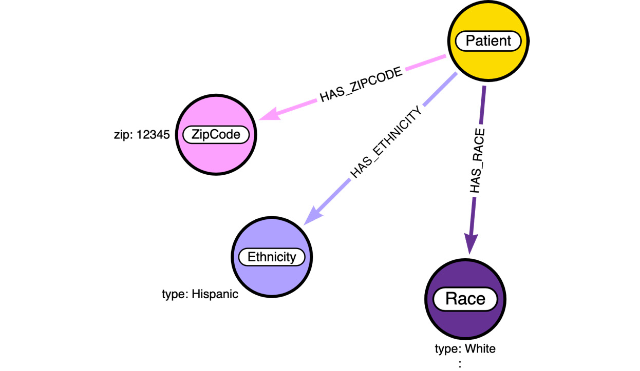
Figure 3.6 – Data diagram with patient data

We can see here that we have chosen to create a Patient node. This is as expected. The Patient node will have the following properties:

• Id
• marital
• ssn
• firstName
• lastName
• suffix
• prefix
• city
• county
• location (LAT and LON)
• drivers
• birthDate

Most of the properties, such as first name, last name, and so on, are natural properties of the node. The county and city values can be either nodes or properties. It depends on how we would like to query the data. When the city is a property, the value is duplicated on all the nodes with that city value. If we make the city a node, then we will have a single city node, but all the nodes that have this city would be connected via a relationship. We will discuss what option would be better in later sections. The advantage with Neo4j is that say we have something as a property – we can easily convert it into a node or relationship later without having too much impact on the database and client applications.

ZipCode is chosen to be a node by itself. This helps us in providing statistics and seeing aspects of provider and patient interactions in a more performant manner. For the same reason, both Race and Ethnicity are nodes instead of properties.

First, we need to make sure we define the indexes and constraints before we load the data. This is very important as the data grows – without indexes, the data load performance will start degrading.

The following code segment shows the indexes and constraints that are required before we can load the patient data:

CREATE CONSTRAINT patient_id IF NOT EXISTS
FOR (n:Patient)
REQUIRE n.id IS UNIQUE ;
CREATE CONSTRAINT zipcode_id IF NOT EXISTS
FOR (n:ZipCode)
REQUIRE n.zip IS UNIQUE ;
CREATE CONSTRAINT race_id IF NOT EXISTS
FOR (n:Race)
REQUIRE n.type IS UNIQUE ;
CREATE CONSTRAINT eth_id IF NOT EXISTS
FOR (n:Ethnicity)
REQUIRE n.type IS UNIQUE ;

In this case, we have created constraints, as we know these values are distinct. This makes sure we don’t create multiple nodes with the same values and it also gives the query planner enough details to execute the query efficiently.

Now that we have created indexes and constraints, the following code segment shows the Cypher query to load the data from the browser. We have chosen to use the LOAD CSV option to load the data:

:auto LOAD CSV WITH HEADERS from "https://raw.githubusercontent.com/PacktPublishing/Cypher-Querying/main/data/csv/patients.csv" as row
CALL {
  WITH row
  MERGE(p:Patient {id: row.Id})
  SET
    p.marital = row.MARITAL,
    p.ssn = row.SSN,
    p.firstName = row.FIRST,
    p.lastName = row.LAST,
    p.suffix = row.SUFFIX,
    p.prefix = row.PREFIX,
    p.city = row.CITY,
    p.county = row.COUNTY,
    p.location = point({latitude:toFloat(row.LAT), longitude:toFloat(row.LON)}),
    p.drivers=row.DRIVERS,
    p.birthDate=date(row.BIRTHDATE)
  WITH row,p
  MERGE (r:Race {type: row.RACE})
  MERGE (p)-[:HAS_RACE]->(r)
  WITH row,p
  MERGE (e:Ethnicity {type: row.ETHNICITY})
  MERGE (p)-[:HAS_ETHNICITY]->(e)
  WITH row,p
  WHERE row.ZIP IS NOT NULL
  MERGE (z:ZipCode {zip: row.ZIP})
  MERGE (p)-[:HAS_ZIPCODE]->(z)
 } IN TRANSACTIONS OF 1000 ROWS

The first thing we can notice here is the usage of the :auto keyword. This is not a Cypher keyword. This is a browser helper keyword that tells the browser to create a single transaction to execute the query. This keyword is used only with the browser and cannot be used anywhere else.

The next thing we can notice is that once the row is read from CSV, we are using this Cypher code segment to execute the query:

CALL {
  …
} IN TRANSACTIONS OF 1000 ROWS

The preceding code segment shows the new batch processing syntax introduced in 4.4 onward. This optimizes the use of transactions. Before 4.4, you needed to use the apoc.load.csv method to load the data this way. Alternatively, you can also use the USE PERIODIC COMMIT Cypher keyword before 4.4 to load the data in batches:

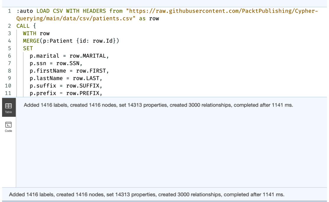
Figure 3.7 – LOAD CSV for patients.csv

This screenshot shows the results after running the query in the browser. You can see that it shows the total number of nodes, relationships created, and number of properties set.

Next, we will take a look at loading the encounters.csv file.

Loading the encounter data

The encounter data represents patient interactions with the healthcare system, whether a lab encounter, doctor visit, or hospital visit. The data available provides a rich set of information. We will only be ingesting part of the information into a graph.

We will only be ingesting the values for the keys identified here from the CSV file:

• Id
• Start
• Patient
• Organization
• Provider
• EncounterClass
• Code
• Description

We are ignoring the cost details as well as the payer details for this exercise. It might be too overwhelming to review and represent all the data. For that purpose, we are limiting what data we are planning to load to do basic patient analysis.

If we add the encounter data representation to the existing patient data diagram, it could look like this:

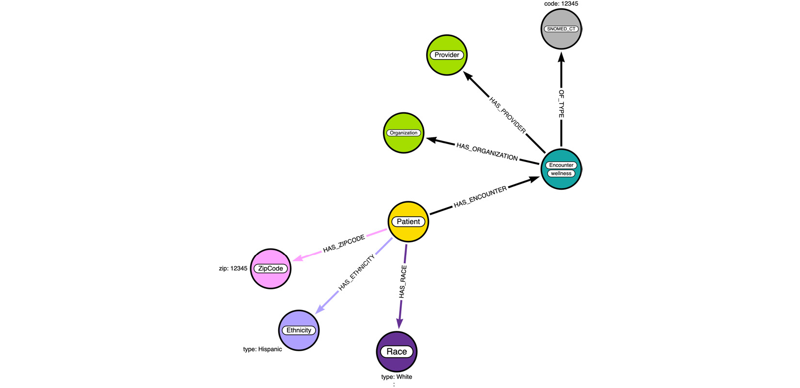
Figure 3.8 – Data diagram enhanced with encounter data

In the diagram, we see an Encounter node as expected. We can notice that this node has an extra label, wellness, on it. We have chosen to represent the EncounterClass value as a label instead of a property. In Neo4j, doing this can make it easier to build performant queries.

Say we want to count all the wellness encounters. When we make it a label, the database can return the count very quickly, as label stores contain statistics related to that node type. The performance remains constant irrespective of how many encounter nodes exist. If we have it as a property and we do not have an index on that property, as the number of encounter nodes grows, the query response time will keep increasing. If we add an index, then we will be using index storage and the performance will be better than not having an index, but still, it has to count using the index store. This topic will be discussed further with examples in later sections.

The Organization, Provider, and SNOMED_CT nodes represent the information this encounter is associated with. We have only the reference IDs for Organization and Provider in the data, so they should be nodes by themselves, similar to how foreign keys are used in the RDBMS world. We have chosen to make code a separate node, as it is industry-standard SNOMED_CT code. By making it a node, we might be able to add extra information that can help with data analysis.

The following code segment shows the Cypher code to create the indexes and constraints needed before ingesting the encounter data:

CREATE INDEX encounter_id IF NOT EXISTS
FOR (n:Encounter)
 ON n.id

We have chosen to use an index here instead of a constraint for encounters. When we are ingesting the other data, the reason for this will become more apparent. We are going to use the following code segment to create the constraints required to load the encounter data:

CREATE CONSTRAINT snomed_id IF NOT EXISTS
FOR (n:SNOMED_CT)
 REQUIRE n.code IS UNIQUE ;
CREATE CONSTRAINT provider_id IF NOT EXISTS
FOR (n:Provider)
 REQUIRE n.id IS UNIQUE ;
CREATE CONSTRAINT organization_id IF NOT EXISTS
FOR (n:Organization)
 REQUIRE n.id IS UNIQUE ;

The following Cypher snippet loads the encounter data into a graph:

:auto LOAD CSV WITH HEADERS from "https://raw.githubusercontent.com/PacktPublishing/Cypher-Querying/main/data/csv/encounters.csv" as row
CALL {
  WITH row
  MERGE(e:Encounter {id: row.Id})
  SET
    e.date=datetime(row.START),
    e.description=row.DESCRIPTION,
    e.isEnd = false
  FOREACH (ignore in CASE WHEN row.STOP IS NOT NULL AND row.STOP <> '' THEN [1] ELSE [] END |
          SET e.end=datetime(row.STOP)
  )
  FOREACH (ignore in CASE WHEN row.CODE IS NOT NULL AND row.CODE <> '' THEN [1] ELSE [] END |
    MERGE(s:SNOMED_CT {code:row.CODE})
    MERGE(e)-[:OF_TYPE]->(s)
  )
  WITH row,e
  CALL apoc.create.setLabels( e, [ 'Encounter', row.ENCOUNTERCLASS ] ) YIELD node
  WITH row,e
  MERGE(p:Patient {id: row.PATIENT})
  MERGE (p)-[:HAS_ENCOUNTER]->(e)
  WITH row,e
  MERGE (provider:Provider {id:row.PROVIDER})
  MERGE(e)-[:HAS_PROVIDER]->(provider)
  FOREACH (ignore in CASE WHEN row.ORGANIZATION IS NOT NULL  AND row.ORGANIZATION <> '' THEN [1] ELSE [] END |
     MERGE (o:Organization {id: row.ORGANIZATION})
     MERGE (e)-[:HAS_ORGANIZATION]->(o))
 } IN TRANSACTIONS OF 1000 ROWS

In this code, you can see there is a new pattern in which FOREACH is introduced. FOREACH is normally used to iterate a list and add or update the data in a graph.

Let’s take a step-by-step look at one of these statements used in the preceding code block that uses a FOREACH clause to simulate an IF condition, which does not exist in Cypher. The code block that we are exploring is shown here:

FOREACH (
    ignore in
    CASE
        WHEN row.CODE IS NOT NULL AND row.CODE <> ''
        THEN
            [1]
        ELSE
            []
    END |
        MERGE(s:SNOMED_CT {code:row.CODE})
        MERGE(e)-[:OF_TYPE]->(s)
)

The execution flow of the preceding code segment can be described with these steps:

1. First, we are using a CASE statement to check for a condition.
2. The WHEN clause is checking for the condition.
3. If the condition is true, the THEN clause will activate and return a list with one value, [1].
4. If the condition is false, the ELSE clause will activate and return an empty list, [].
5. We are iterating the list returned and assigning it to a variable, ignore.
6. If the list is not empty, then the ignore variable will be assigned to the value in the list, which contains one element, 1 and will process the set of statements after the | separator. We are calling this variable ignore as we don’t need to know what value this holds. We want to execute what’s after the | separator exactly once if the condition is true.

This is how we can simulate the IF condition in Cypher. If you want IF and ELSE conditional execution, then you have to use apoc procedures.

Also, we are using the apoc procedure to add EncounterClass to an encounter node. Since we are trying to add labels dynamically, we have to use the apoc option:

CALL apoc.create.setLabels( e, [ 'Encounter', 
    row.ENCOUNTERCLASS ] ) YIELD node

In Cypher, it is not possible to set the label with a dynamic value.

Next, we will take a look at ingesting provider data.

Loading provider data

The provider data represents the physicians that participate in the healthcare system. We will be using all the data provided except the utilization value.

After adding the provider data details, our data diagram will look like this:

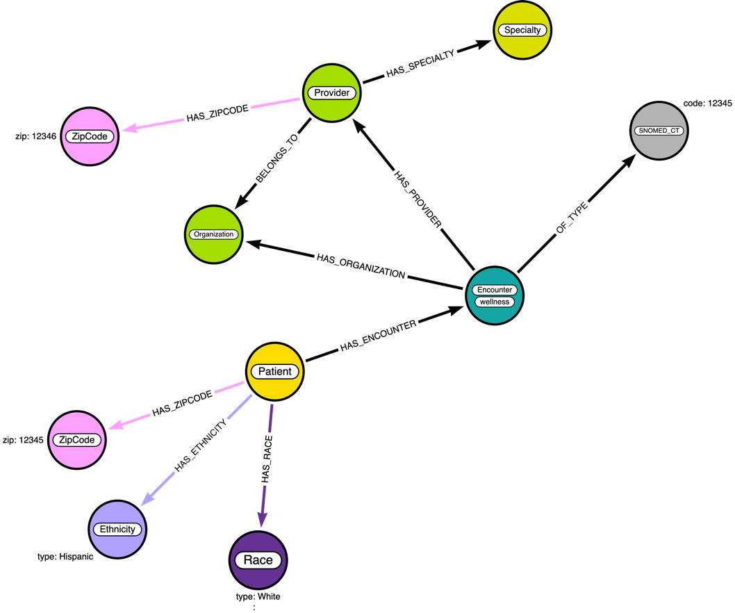
Figure 3.9 – Data diagram enhanced with provider data

We have a new Specialty node added. We have new relationships added between the Provider, Organization, and ZipCode nodes. By making Speciality a node, it can make it easier to group Provider nodes in queries.

Since we introduced a new label type, we need to add an index or a constraint for this. The code segment here shows the Cypher code for this:

CREATE CONSTRAINT specialty_id IF NOT EXISTS
FOR (n:Specialty)
REQUIRE n.name IS UNIQUE

The following Cypher code loads the provider data into a graph:

:auto LOAD CSV WITH HEADERS from "https://raw.githubusercontent.com/PacktPublishing/Cypher-Querying/main/data/csv/providers.csv" as row
CALL {
  WITH row
  MERGE (p:Provider {id: row.Id})
  SET p.name=row.NAME,
      p.gender=row.GENDER,
      p.address = row.ADDRESS,
      p.state = row.STATE,
      p.location = point({latitude:toFloat(row.LAT), longitude:toFloat(row.LON)})
  WITH row,p
  MERGE (o:Organization {id: row.ORGANIZATION})
  MERGE(p)-[:BELONGS_TO]->(o)
  WITH row,p
  MERGE (s:Specialty {name: row.SPECIALITY})
  MERGE (p)-[:HAS_SPECIALTY]->(s)
  WITH row,p
  WHERE row.ZIP IS NOT NULL
  MERGE (z:ZipCode {zip: row.ZIP})
  MERGE (p)-[:HAS_ZIPCODE]->(z)
 } IN TRANSACTIONS OF 1000 ROWS

Here, we are using a different approach to conditional execution. For providers, the ZIP code value is optional and since we are processing the ZIP code, in the end, we can use a WHERE clause alongside a WITH clause:

  WITH row,p
  WHERE row.ZIP IS NOT NULL

When we use this approach, the query execution continues only when the ZIP value is not null. This can only work when the conditional check is the last one. If we do this in between, all the logic below this will not get executed if the ZIP value is null.

Next, we will load the organization data.

Loading organization data

The organization data represent the hospitals or labs. We will be loading all the values except the Revenue and Utilization values into the graph.

After adding the organization data details, our data diagram will look like this:

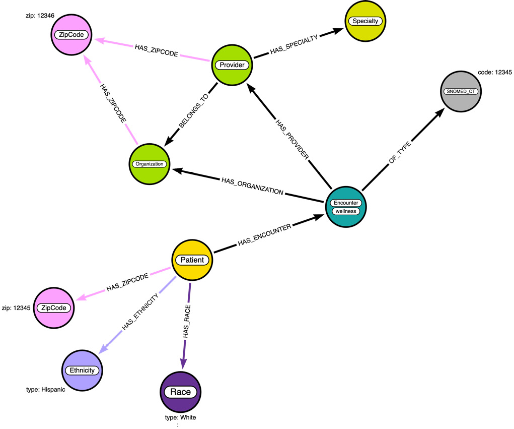
Figure 3.10 – Data diagram enhanced with organization data

Here, we did not introduce any new node types. The only change to the diagram is the presence of a new relationship between Organization and ZipCode.

The following Cypher code loads the organization data into a graph:

:auto LOAD CSV WITH HEADERS from "https://raw.githubusercontent.com/PacktPublishing/Cypher-Querying/main/data/csv/organizations.csv" as row
CALL {
  WITH row
  MERGE (o:Organization {id: row.Id})
  SET o.name=row.NAME,
      o.address = row.ADDRESS,
      o.state = row.STATE,
      o.location = point({latitude:toFloat(row.LAT), longitude:toFloat(row.LON)})
  WITH row,o
  WHERE row.ZIP IS NOT NULL
  MERGE (z:ZipCode {zip: row.ZIP})
  MERGE (o)-[:HAS_ZIPCODE]->(z)
 } IN TRANSACTIONS OF 1000 ROWS

This is pretty much similar to the provider data load. We are creating or updating organization data and connecting it to a ZIP code when it is available.

Next, we will take a look at loading medication data.

Loading medication data

The medication data represents the drugs prescribed to the patient. From medication data, we will be using these values:

• Patient
• START
• STOP
• Encounter
• CODE
• DESCRIPTION
• REASONCODE
• REASONDESCRIPTION

As you can see here, we want to represent the START and STOP values of medication in the graph. If we just make them properties on the node, then we will lose the timing context of the patient encounters. To make sure we preserve the timing context, we might create a new Encounter node with the same Encounter ID and STOP time as the distinct values. If you remember, only for the Encounter node did we add an index on id, whereas for almost all the other entities, we created a constraint. This makes START and STOP distinct entities in the graph and can help in analyzing the data.

After adding the organization data details, our data diagram will look like this:

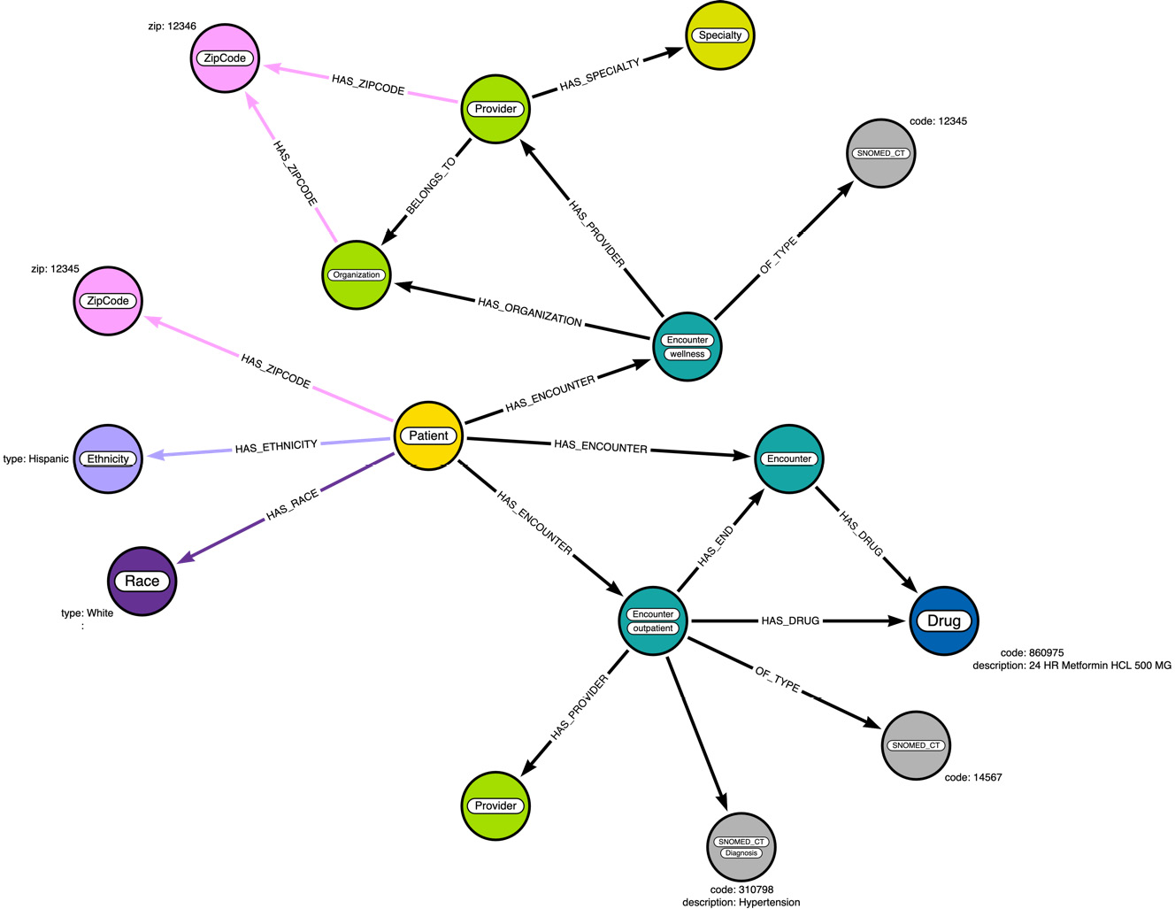
Figure 3.11 – Data diagram enhanced with medication data

From the data diagram, we can see the model getting more complex as more and more context is ingested into the graph. Especially the addition of a new Encounter node and the HAS_END relationship are a bit different from how we approach the data in the RDBMS world. This can assist us in analyzing how a drug being used could have an effect on patient health.

The following Cypher code loads the medication data into a graph:

:auto LOAD CSV WITH HEADERS from "https://raw.githubusercontent.com/PacktPublishing/Cypher-Querying/main/data/csv/medications.csv" as row
CALL {
  WITH row
  MERGE (p:Patient {id:row.PATIENT})
  MERGE (d:Drug {code:row.CODE})
    SET d.description=row.DESCRIPTION
  MERGE (ps:Encounter {id:row.ENCOUNTER, isEnd: false})
  MERGE (ps)-[:HAS_DRUG]->(d)
  MERGE (p)-[:HAS_ENCOUNTER]->(ps)
  FOREACH( ignore in CASE WHEN row.REASONCODE IS NOT NULL AND row.REASONCODE <> '' THEN [1] ELSE [] END |
    MERGE(s:SNOMED_CT {code:row.CODE})
      SET s:Diagnosis, s.description = row.REASONDESCRIPTION
    MERGE (ps)-[:HAS_DIAGNOSIS]->(s)
  )
  WITH row,ps,p
  WHERE row.STOP IS NOT NULL and row.STOP <> ''
  CREATE (pe:Encounter {id:row.ENCOUNTER, date:datetime(row.STOP)})
    SET pe.isEnd=true
  CREATE (p)-[:HAS_ENCOUNTER]->(pe)
  CREATE (pe)-[:HAS_DRUG]->(d)
  CREATE (ps)-[:HAS_END]->(pe)
 } IN TRANSACTIONS OF 1000 ROWS

Here, we can see that when there is an underlying condition for the drug prescribed, we are creating a SNOMED_CT node, but adding the Diagnosis label on it. This is the same approach we had used with Encounter class values.

In the code, to create the new Encounter node to represent the Stop value, we are using the CREATE clause. This can be very performant, but the negative effect is that when we process this data again, say by mistake, we are going to create duplicate nodes. We are going to look at using MERGE with a Stop timestamp in the next data file processing. You would need to decide which approach would suit your data ingestion needs better.

Next, we will look at loading condition, procedure, and allergy data.

Loading condition, procedure, and allergy data

The data loading is pretty similar to the medication data. Even the data diagram won’t alter much. The pattern would be pretty similar to the drug data.

After adding these data details, our data diagram will look like this:

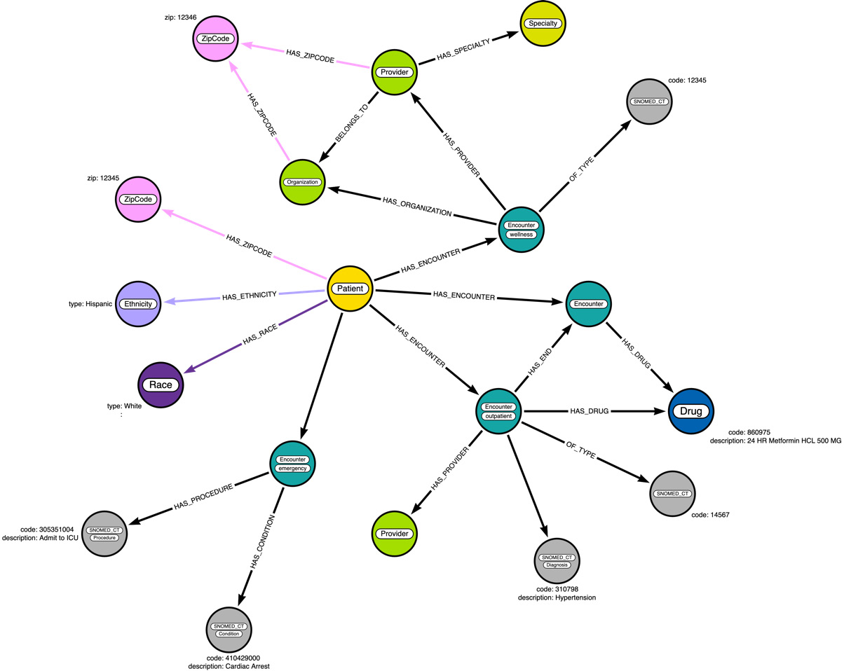
Figure 3.12 – Data diagram enhanced with condition, procedure, and allergy data

We will add two more relationships, HAS_CONDITION and HAS_PROCEDURE. We have not represented the HAS_END relationship here:

• The following Cypher code loads the condition data into a graph:

  :auto LOAD CSV WITH HEADERS from "https://raw.githubusercontent.com/PacktPublishing/Cypher-Querying/main/data/csv/conditions.csv" as row

  CALL {

    WITH row

    MATCH (p:Patient {id:row.PATIENT})

    MERGE (c:SNOMED_CT {code:row.CODE})

    SET c.description=row.DESCRIPTION, c:Condition

    MERGE (cs:Encounter {id:row.ENCOUNTER, isEnd: false})

    ON CREATE

      SET cs.date=datetime(row.START)

    MERGE (p)-[:HAS_ENCOUNTER]->(cs)

    MERGE (cs)-[:HAS_CONDITION]->(c)

    WITH p,c,cs,row

    WHERE row.STOP IS NOT NULL and row.STOP <> ''

    MERGE (ce:Encounter {id:row.ENCOUNTER, date:datetime(row.STOP)})

    SET ce.isEnd=true

    MERGE (p)-[:HAS_ENCOUNTER]->(ce)

    MERGE (ce)-[:HAS_CONDITION]->(c)

    MERGE (cs)-[:HAS_END]->(ce)

   } IN TRANSACTIONS OF 1000 ROWS

In this code, we can see that for a condition, we are also adding a SNOMED_CT node with a Condition label added to it. We also have a MERGE clause here to add to the Encounter node to represent the STOP condition.

• The following Cypher code loads the procedure data into a graph:

  :auto LOAD CSV WITH HEADERS from "https://raw.githubusercontent.com/PacktPublishing/Cypher-Querying/main/data/csv/procedures.csv" as row

  CALL {

    WITH row

    MATCH (p:Patient {id:row.PATIENT})

    MERGE (c:SNOMED_CT {code:row.CODE})

    SET c.description=row.DESCRIPTION, c:Procedure

    MERGE (cs:Encounter {id:row.ENCOUNTER, isEnd: false})

    ON CREATE

      SET cs.date=datetime(row.START)

    MERGE (p)-[:HAS_ENCOUNTER]->(cs)

    MERGE (cs)-[:HAS_PROCEDURE]->(c)

   } IN TRANSACTIONS OF 1000 ROWS

We can see the ingestion of data is simple.

• The following Cypher code loads the allergy data into a graph:

  :auto LOAD CSV WITH HEADERS from "https://raw.githubusercontent.com/PacktPublishing/Cypher-Querying/main/data/csv/allergies.csv" as row

  CALL {

    WITH row

    MATCH (p:Patient {id:row.PATIENT})

    MERGE (c:SNOMED_CT {code:row.CODE})

    SET c.description=row.DESCRIPTION, c:Allergy

    MERGE (cs:Encounter {id:row.ENCOUNTER, isEnd: false})

    ON CREATE

      SET cs.date=datetime(row.START)

    MERGE (p)-[:HAS_ENCOUNTER]->(cs)

    MERGE (cs)-[:ALLERGY_STARTED]->(c)

    WITH p,c,cs,row

    WHERE row.STOP IS NOT NULL. and row.STOP <> ''

    MERGE (ce:Encounter {id:row.ENCOUNTER, date:datetime(row.STOP)})

    SET ce.isEnd=true

    MERGE (p)-[:HAS_ENCOUNTER]->(ce)

    MERGE (ce)-[:ALLERGY_ENDED]->(c)

    MERGE (cs)-[:HAS_END]->(ce)

   } IN TRANSACTIONS OF 1000 ROWS

We can see we are following the exact same pattern as with conditions. Here, we are capturing the STOP aspect, as it might be useful for analysis purposes.

Next, we will take a look at loading care plan data.

Loading care plan data

Care plan data contains the care schedule associated with a patient. It follows the same pattern as the medication or condition data loading process.

After adding these data details, our data diagram will look like this:

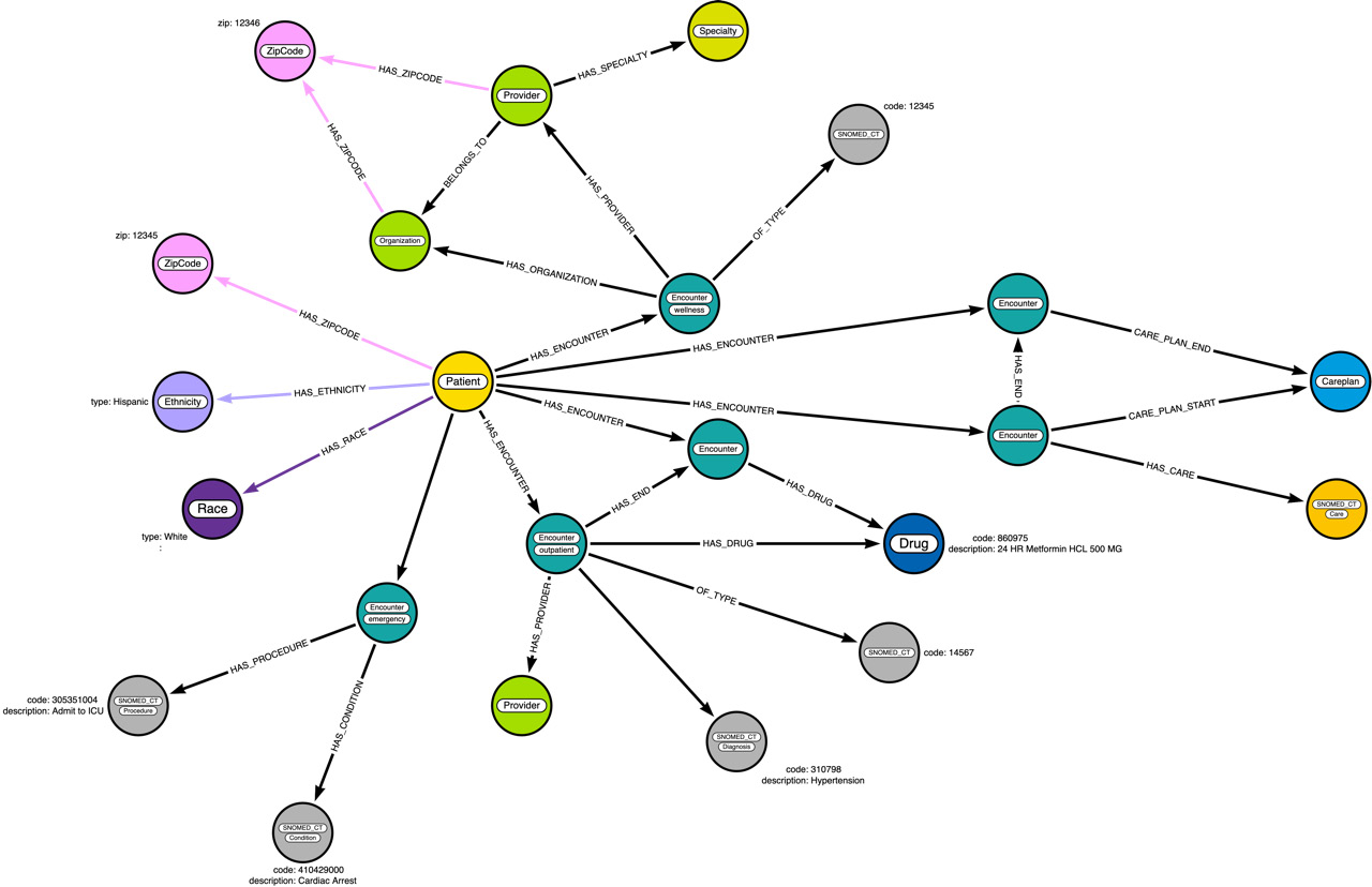
Figure 3.13 – Data diagram enhanced with care plan data

We can see that we are seeing more nodes, but the pattern those nodes follow is similar. Our graph data model is not too complex. We will take a look at how Neo4j interprets the graph data model in the next section.

The following Cypher code loads the procedure data into a graph:

:auto LOAD CSV WITH HEADERS from "https://raw.githubusercontent.com/PacktPublishing/Cypher-Querying/main/data/csv/careplans.csv" as row
CALL {
  WITH row
  MATCH (p:Patient {id:row.PATIENT})
  MERGE (cp:CarePlan {code:row.Id})
  MERGE (c:SNOMED_CT {code:row.CODE})
  SET c.description=row.DESCRIPTION, c:Care
  SET c.description=row.DESCRIPTION
  MERGE (cp)-[:HAS_CARE_TYPE]->(c)
  MERGE (cs:Encounter {id:row.ENCOUNTER, isEnd: false})
  ON CREATE
    SET cs.date=datetime(row.START)
  MERGE (cs)-[:HAS_CARE_TYPE]->(c)
  MERGE (p)-[:HAS_ENCOUNTER]->(cs)
  MERGE (cs)-[:CARE_PLAN_START]->(cp)
  WITH p,cp,cs,row
  WHERE row.STOP IS NOT NULL and row.STOP <> ''
  CREATE (ce:Encounter {id:row.ENCOUNTER, date:datetime(row.STOP)})
  SET ce.code=row.CODE, ce.isEnd=true
  MERGE (p)-[:HAS_ENCOUNTER]->(ce)
  MERGE (ce)-[:CARE_PLAN_END]->(cp)
  MERGE (cs)-[:HAS_END]->(ce)
 } IN TRANSACTIONS OF 1000 ROWS

We can see from the Cypher code that it follows the same pattern as medication data and others.

Now that we have seen the whole data loaded using LOAD CSV, next, we will take a brief look at how we can do the same thing using the client driver.

Using client drivers

While LOAD CSV is convenient, it is not recommended for production usage, so when you have data that needs to be loaded at regular intervals or as a stream, you will need to leverage the client drivers to be able to load the data.

Here, we will take a look at a simple Python client that can load the data into Neo4j using Python drivers. The utility is called pyingest (https://github.com/neo4j-field/pyingest/tree/parquet). This utility can load CSV, JSON, or Parquet data from a local filesystem, from a URL, or an S3 bucket. The whole loading process is controlled by a configuration file, which is in YML format.

The following parameters can be configured in the configuration YML file:

• server_uri: Address of the Neo4j driver (required).
• admin_user: Username of the Neo4j user (required).
• admin_pass: Password for the Neo4j user (required).
• pre_ingest: List of Cypher statements to be run before the file ingests.
• post_ingest: List of Cypher statements to be run after the file ingests.
• files: Describes the ingestion of a file – one stanza for each file. If a file needs to be processed more than once, just use it again in a separate stanza. We will discuss parameters for files now.

File-related configuration options are as follows:

• url: Path to the file (required).
• cql: Cypher statement to be run (required).
• chunk_size: Number of records to batch together for ingest (default: 1,000).
• type: Type of file being ingested (either CSV or JSON). This parameter is not required. If missing, the script will guess based on the file extension, defaulting to CSV.
• field_separator: The character separating values in a line of CSV (the default is ,)
• compression: The type of compression used on a file (either gzip, zip, or none – the default is none)
• skip_file: If true, do not process this file (either true or false – the default is false)
• skip_records: Skips a specified number of records while ingesting the file (the default is 0)

Here, we are including the YML configuration file (https://github.com/PacktPublishing/Cypher-Querying/blob/main/data/config.yml) so that you can try it out yourself.

Once you download the file, you can run the following command to load the data:

Python3 ingest.py config.yml

We can see how having a script like this to load the data can simplify our data load process instead of running LOAD CSV commands one by one from the browser.

Summary

In this chapter, we have seen how we can map the data to graph model using Arrows.app (https://arrows.app/#/local/id=jAGBmsu828g36qjzMAG4), along with working with the browser to load the data using LOAD CSV commands. Along the way, we looked at when to make a value a property or a node or use it an extra label that makes understanding our data much easier in a graph format.

We also discussed various commands for conditional data loading, such as using FOREACH to simulate an IF condition. We also looked at conditional data loading by combining a WHERE clause with a WITH clause.

Along the way, we discussed how the graph data model evolves as we keep considering more data being added to the database. This is made possible since Neo4j is a schemaless database. In a schema-strict database such as an RDBMS, we have to think through all the aspects of the data model before we can attempt to ingest the data. This makes data modeling iterations simpler and gives us the opportunity to tune the model as we understand the data nuances more.

At the end of this chapter, we discussed loading the data using a Python client in a more automated way, rather than the step-by-step approach we have used with LOAD CSV.

In the next chapter, we will look at the graph model that is inferred by Neo4j and will try a few queries to understand how we can query the graph and retrieve it efficiently.