
Script, function files and some useful MATLAB® functions
The commands discussed in previous chapters were executed in the Command Window; they were not saved, and cannot be re-used. Another disadvantage of the Command Window is that correction is possible only on the last line executed.
When one of the sequence commands needs to be corrected, all its predecessors have to be re-executed and the command then corrected, after which all subsequent commands must be repeated to obtain the final result. Moreover, every time a calculation needs to be repeated, all commands have to be retyped and re-entered. This is inconvenient, and the reader who has perused the preceding chapters has undoubtedly experienced it. The remedy lies in writing all commands sequentially into a file, saving it and running it as necessary. MATLAB® has two types of files: script and function files. These types are explained further below. In addition, some MATLAB® functions of numerical analysis that are frequently used in applied calculations are presented.
4.1 Script files
4.1.1 Creation, saving and running
A script file is a sequence of commands (often called a program) that should be run. MATLAB® executes commands in the order they were written. Corrections can be entered directly in the file and new commands can be added. The extension of the saved script file is ‘.m’, hence the term m-files.
A script file should be typed and edited into a MATLAB® Editor. To open the Editor, the command edit should be typed and entered in the Command Window, or the ‘New’ and ‘M-file’ options in the ‘File’ menu should be selected. After this the Editor Window appears (Figure 4.1):
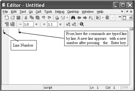
The commands of the script file should be typed line by line. It is also possible to type two or more commands on the same line, dividing them by commas or by semicolons. A new line will be accessible after pressing the Enter key. Each new line is numbered automatically. A command can also be typed in another editor and then copied into the Editor Window.
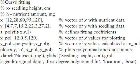
Figure 4.2 on p. 97 shows an elementary script file typed into the Editor Window. The first lines are usually explanatory comments, preceded by the comments sign % and in green (light gray here); they are not part of the execution. The commands appear in black for better legibility.
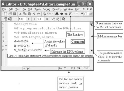
In the latest MATLAB® version the Editor Window appears with a message bar (located on the right) of the so-called M-Lint analyzer, which detects possible errors, comments on them and recommends modifications for better program performance. The bar is topped by the message indicator![]() . A green indicator means no errors, warnings or possibility of improvements; a red indicator means syntax errors have been detected; and an orange indicator means warnings or possibility of improvements (but no errors). When the analyzer detects an error or possibility of improvement, it underlines/highlights the text and a horizontal line appears on the message bar. When the cursor is placed at this line the comment message appears (see Figure 4.2). The changes it recommends – such as the one shown in this figure (addition of a semicolon) – need not be executed because we want to display the resulting value of the DNA volume, V_DNA. The M-Lint regime appears in the Editor Window by default and can be disabled by un-signing the ‘Enable integrated M-Lint warning and error messages’ check-box in the M-Lint option of the Preferences Window, which can be selected from the File in the Editor Window or in the Desktop menu.
. A green indicator means no errors, warnings or possibility of improvements; a red indicator means syntax errors have been detected; and an orange indicator means warnings or possibility of improvements (but no errors). When the analyzer detects an error or possibility of improvement, it underlines/highlights the text and a horizontal line appears on the message bar. When the cursor is placed at this line the comment message appears (see Figure 4.2). The changes it recommends – such as the one shown in this figure (addition of a semicolon) – need not be executed because we want to display the resulting value of the DNA volume, V_DNA. The M-Lint regime appears in the Editor Window by default and can be disabled by un-signing the ‘Enable integrated M-Lint warning and error messages’ check-box in the M-Lint option of the Preferences Window, which can be selected from the File in the Editor Window or in the Desktop menu.
The script file should be saved after it has been written into the Editor Window. For this the ‘Save As …’ option from the File menu should be chosen. After this the ‘Save file as …’ window appears and the desired file location and file name should be typed respectively into the ‘Save in:’ and ‘File name:’ positions. By default the ‘MATLAB’ subdirectory in the ‘My documents’ directory is automatically selected for the file location, or the desired directory has to be chosen from the pop-up menu which appears after pressing on the arrow on the right-hand side of the ‘Save in:’ field of the ‘Save file as …’ window. The name for a script file should begin with a letter, and should not repeat the user-defined or predefined variables, MATLAB® commands or functions. In addition, it is not recommended to introduce spaces into the name, which cannot be longer than 63 characters.
To execute a script file: first, the user should check the current MATLAB directory, and if the file is not in it a directory with this file should be set; secondly, the file name should be typed in the Command Window and then entered.
Current directory
The currently set directory is shown in the ‘Current Folder’ field of the MATLAB® Desktop (see Figure 4.3). The simplest way to achieve the desired setting is:
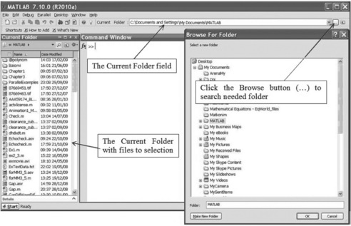
• click on the icon with three points ![]() on the right-hand side of the Current Folder field, after which the Browse for Folder Window appears;
on the right-hand side of the Current Folder field, after which the Browse for Folder Window appears;
• select and click on the desired directory which appears in the Current Folder field.
For example, the script file with name EditorExample1.m (Figure 4.2) was saved in the Chapter 4 folder and located on disk D. To run it we need to change the current directory to D:Chapter4 in the described way, type the file name (without the m-extension) in the Command Window, and then press the Enter key (p.117, top).
> > runs the script file with the name EditorExample1
The result of calculations via the commands is saved in the script file, and is displayed in the Command Window.
4.1.2 Input values to variables of a script file
To assign a value to the variables defined in the script file when the script is run the input command should be used; this command has the forms:
Numeric_Variable_Name = input('Displayed string') Character_Variable_Name = input('Displayed string','s')
where 'Displayed string' is a text that displays in the Command Window and prompts us to assign a number to the Numeric_Variable_ Name, or a string to the Character_Variable_Name; 's' indicates that inputting characters are string.
After running a script file, when the input command is started, the string written in this command appears on the screen and the user should type and enter a number or string; inputted values are assigned to the Numeric_Variable_Name or to the Character_Variable_Name depending on the command form used.
As an example is a command script file that convert a weight, g_lb, in pounds to kilograms, g_kg, by the expression g_kg = g_lb/2.2046:
The file is saved with the pound2kg name. After typing and entering this file name in the Command Window, the prompt ‘Enter your weight in pounds, G =’ appears on the screen, a weight value should be typed (in pounds) after the sign ‘=’ and enter pressed; the weight is converted to kilograms and displayed on the screen. The run command, prompts, and input and output numbers are:
With the input command the vectors and matrices can be inputted in the same way as for a variable – numbers in square brackets.
4.2 Functions and function files
4.2.1 Creating the function
In algebra a function is presented as the equation y = f(x), whose right-hand side contains one – x – or more parameters (arguments) – x or x, a, b, …. When these parameters are assigned, the value of y is obtained. Similarly to the above, many MATLAB® commands discussed in the preceding chapters are written in function form, sin(x), cos(x), log(x), sqrt(x), etc., and can be used for direct calculations or placed into more complicated expressions by typing their name with the argument. In MATLAB® it is possible to create any new function and re-use it with different argument values and in different programs; such functions are termed ‘user-defined’. Not only a specific expression, but a complete program created by the user can be defined as a function and saved as a function file. The MATLAB® definition of a function reads
function[output_parameters] = function_name(input_parameters)
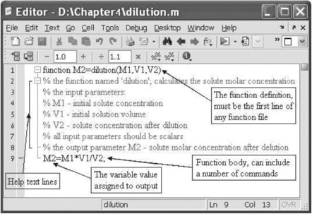
The word function appears in blue and must be the first word in the file. The function name is written to the right of the ‘=’ sign and should obey the same rules as for variable names (see subsection 2.1.4). As input_ parameters we should write a list of arguments for transfer into the function, and as output_parameters a list of those we want to derive from the function. The input parameters must be written in parentheses and the output parameters in square brackets. (In the case of a single output parameter the brackets can be dispensed with.) Parameters must be divided by commas.
As with a script file, a function file should be written in the Editor Window. An example of a function file is presented in Figure 4.4 on p. 101. This function is named dilution and calculates the molar concentration of a solute after dilution. It has three input parameters – the molar concentration M1 and the solution volume V1 before dilution, and solution volume V2 after dilution – and one output parameter – the molar concentration of the solute after dilution.
The requirements and recommendations regarding the structure and certain parts of the function file are:
Line with the function definition
In addition to the previous comments regarding the function definition, the function can be written with the parameters omitted completely or in part. Possible variants of the function definition line are given in the following examples:
| function [A,B] = example1(a,b,c) | full record, function name ‘example1’, three input and two output parameters; |
| function [A,B,C] = example2 | function without input parameters, function name ‘example2’, three output parameters; |
| function example3(a,b,c) | function without output parameters, function name ‘example3’, three input parameters. |
| function example4 | the function without parameters, function name ‘example4’. |
Number and names of the input and output parameters can differ from those in the examples. The word ‘function’ should be written in lower-case letters.
Lines with help comments
These lines are placed just after the function definition line and before the first non-comment line. The first of these lines should contain a short definition of the function (used by the lookfor command when it searches the information). The help comments are displayed when the help command is introduced with the user-defined function name; for example, typing into the Command Window help dilution yields:
Lines of function body, local and global variables
The function body can contain one or more commands for actual calculations; between these commands, usually at their end, should be placed the assignments to the output parameters; for example, in the example in Figure 4.4 the output parameter is M2 and the last command calculates and assigns the found value to M2. The actual values must be assigned to the input parameters before running the function.
The variables in the function file are local and relevant only within the file. This means that once the function has been run, the variables are not saved and no longer appear in the workspace. If we want to share some or all of them with other function(s), we should make them accessible, which can be done with the global command in the form
global variable_name1 variable_name2 …
The global command must be written before the variable is first used in the function and also in other functions where it is intended to be used.
4.2.2 Saving a function as a function file
Before a function is used, it must be saved in a file. This is done exactly as for a script file – selecting ‘Save As’ from the File menu and then entering the desired location and name for the file. It is recommended that the file be called by the function name, e.g. the dilute function should be saved in a file named dilute.m.
Examples of function definition lines and function file names:
| function a = fly(h,l) | the function file should be named and saved as fly.m; |
| function [v, m] = dna_r(d,h) | the function file should be dna_r.m; |
| function weights(h) | the function file should be weights.m. |
When a program has two or more functions, the name of a function file should be identical to the name of the main function (from which the program starts).
4.2.3 Running a function file
The function file can be run from another file or from the Command Window as follows. The function file definition line should be typed without the word ‘function’ and the input parameters should be assigned their values. For example, the dilution function file (see Figure 4.4) can be run thus:
Or alternatively with pre-assignment of the input variable:
A user-defined function can be used in another mathematical expression or program; for example, dilution gives M2 solute concentrations in mol/L for V2 = 0.6 L of the solution; thus the solution has M2_mol = M2*V2 moles. For the calculations the following commands should be typed in the Command Window:
> > % defines values for the input parameters in the dilution function
> > M2_mol = c*dilution(a,b,c) % moles in the 0.6 L solution
Comparison of script and function files
First-year students, and life science students in particular, may find it difficult to understand the differences between script and function files, because most of their problems can be solved via the former type, or simply by inputting commands directly into the Command Window. Accordingly, the similarities and differences between these types are outlined below.
• Both are produced with the help of the Editor and saved as m-files (files with the extension m)
• The first line of the function file must be the function definition line
• The name of the function file should be the same as that of the function
• Function files can receive and return data through the input and output parameters, respectively
• Script files require parameters to be written straight into the file or with input commands
• Function files can be used as functions in other MATLAB® files or simply in the Command Window.
4.3 Some useful MATLAB® functions
Biotechnology laboratory practice involves a variety of mathematical operations such as interpolation, extrapolation, solution of algebraic equations, integration, differentiation and fitting. MATLAB® functions that can be used for these purposes are discussed below.
4.3.1 Interpolation and extrapolation
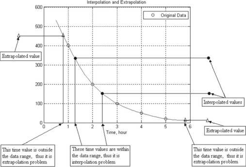
When data are available (by measurement or by tables) at certain points and we need to estimate intermediate values between them, this can be done by interpolation. When values outside the data points need to be evaluated, this can be done by extrapolation. For example, the values of measured radioactive decay R of a liquid substance are 400, 200, 100, 50 and 20 disintegrations per minute at times t = 1, 2, 3, 4 and 5 hours, respectively. The graph with the data points is presented in Figure 4.5. Finding the decay values at t = 1.2 and 2.4 hours (values between data points) is an interpolation problem, and finding them at t = 0.8 and 5.8 hours (values outside data points) is an extrapolation problem.
In MATLAB® both interpolation and extrapolation operations can be done with the interp1 function. This command has the forms
yi = interp1(x,y,xi,'method') or
yi = interp1(x,y,xi,'method','extrap')
The first version is used for interpolation, and the second for extrapolation or for simultaneous interpolation and extrapolation.
The output parameter for these MATLAB® functions is yi – the interpolated value or vector of values. The input parameters are x and y, vectors of data values – argument and function, respectively; xi, a scalar or a vector with the points for which the values of yi are sought; 'method' is the string that contains the name of the mathematical method to be used for interpolation or extrapolation; some available methods are 'linear', 'cubic' and 'spline'; a default method is 'linear', which need not be specified.
The 'extrap' string is required for the 'linear' method; the word can be omitted for the 'cubic' and 'spline' methods.
For the example in Figure 4.5 the commands for interpolation (at points 1.2 and 2.4 hours) and extrapolation (at points 0.8 and 5.8 hours) are:
| > > R = [400, 200, 100, 50, 20]; | % the data for x |
| > > t = 1:5; | % the data for y |
| > > xi = [1.2 2.4]; | % the points of interpolation |
| > > xe = [0.8 5.8]; | % the points of extrapolation |
| > > y_interpolated = interp1 (t,R,xi,'spline'), | % defines interpolated values |
| > > y_extrapolated = interp1 (t,R,xi,'linear','extrap'), | % defines extrapolated values |
| > > display interpolated and extrapolated values | |
| > > y_interpolated,y_extrapolated | |
| y_interpolated = 349.3600 151.0800 | |
| y_extrapolated = 360 160 |
4.3.2 Solution of non-linear algebraic equations
The matrix solution for a set of linear algebraic equations was discussed in chapter 2 (subsections 2.2.2, 2.3.4.1). Here we deal with non-linear equations with iterations in which the computer finds the x value at which f(x) = 0. The function for this process is fzero and its general form is:
The fzero function seeks an x value representing the solution near the guess point x0; and 'fun' is the string function to be solved. In this string the equation itself can be written, or the name of the user-defined function that contains it.
One possible way to determine the approximate value of x0 is to plot the graph of the equation and check the x-value at which the function is zero. For example, consider the Arrhenius equation
where the value k/A = 8.7271 × 10⁻¹⁴ was previously determined at T = 300 K and R = 8.314 J/kmol. The unknown variable is the activation energy E0 and should be named x, and the equation presented in the form ![]() . The value of x0 must be positive for physical reasons and for many reactions it is around 5 × 10⁴ J/mol.
. The value of x0 must be positive for physical reasons and for many reactions it is around 5 × 10⁴ J/mol.
The string with the solved equation cannot include pre-assigned variables; for example, it is not possible to define k/A = 8.7271 × 10⁻¹⁴, R = 8.314, T = 300 K and then write 'k_A-exp(− x/(R*T))'.
For substitution of pre-assigned parameters into the solving expression the following form of fzero is available:
x = fzero(@(x) fun(x, preassigned_variables1, preassigned_variables2,… ), x0)
@(x) fun1 indicates a user-defined function that contains the equation with the additional arguments preassigned variablesl, preassigned variables2, ….
Using this form, we can write the above example as a function file with the name actener, input parameters k/A, R, T and x0, and output parameter E0. In this function file the fzero command reads x = fzero (@ (x) myf(x,k_A,R,T), x0) and the function definition line for the myf function should appear as function f = myf(x,k_A,R,T). The full text of the actener function is
function Eo = actener(k_A, R, T,x0)
% activation energy calculation
Eo = fzero(@ (x) myf(x,k_A,R,T), x0);
This function should be saved as actener.mfile and run into the Command Window with assigned parameters k/A, R, T and x0:
4.3.3 Integration
The area beneath a segment of a function f(x) or beneath data points (Figure 4.6) can be determined by numeric integration. For this the area is subdivided into small geometrical elements, e.g. rectangles and trapezoids. The integral is the sum of the areas of these elements. Below, two MATLAB® functions for integration are described – quad and trapz. The first is used when f(x) is presented as an analytical expression, and the second when it is presented as data points.
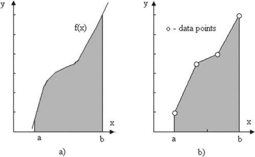
Figure 4.6 Definite integral (the shaded area) of the function f(x) given analytically (a) and by the data points (b).
The quad function
This function uses the adaptive Simpson method and has the form:
where 'function' is a string with the expression f(x) to be integrated, or the name of a function file where the expression should be written (in the same way as for the fzero command); a and b are the integration limits, tol is the desired maximal absolute error (this parameter is optional and can be dispensed with); the default tolerance is smaller than 1 × 10⁻⁶; q is the variable to which the value of the integral obtained is assigned.
The function f(x) should be written using element-wise operators, e.g. ‘.*’, ‘.^’ and ‘./’.
For example, to calculate the integral  (the function 1/x2appears in second-order reaction rates, in population dynamics, etc.) the following command should be typed and entered from the Command Window
| > > q = quad('1./x.^2',1,5) | % Note: the element-wise operations are used for 1/x2 |
| q = 0.8000 |
Another possible way of using quad is to write in the Editor Window and save the function file that contains the function 1/x2:
To integrate the saved function in the Integr_Ex.m file, the quad command should be typed and then entered from the Command Window:
Preassigned parameters can be substituted in the 'function' expression in the same way as for the fzero command.
The trapz function
where x and y are vectors of the point coordinates; the function uses the trapezoid method for numerical integration when the function is presented as data points.
For example, for growth rates of:
![]()
the number N of bacterial cells at the end of the measurements is
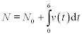
where N0 = 10 is the initial cell number; v(t) under the integral is given numerically in the table. The result, which obviously cannot be a fraction, should be rounded to the nearest lesser integer.
The next command should be typed and entered from the Command Window:
4.3.4 Derivatives
The derivative dy/dt of the function y(t) is characterized by the infinitesimal change in the function at some given point; in geometrical representation (Figure 4.7, p. 111) it is the slope of the tangent to the curve at the ith point (x,t).
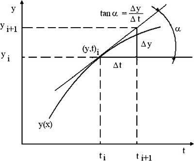
Following these definitions, the derivative can be presented for numerical calculations as:
Thus, the derivative can be calculated at each i-point as the ratio of y- and x-differences between neighboring points. The diff command for these differences has the forms:
dy = diff(y) or dy_n = diff(y,n)
where y is the vector of y-values at points i = 1, 2, …; the n argument indicates how many times the diff command should be applied and the order of the particular difference. For example, if n = 2 the diff command should be applied twice; the dy and dy_n output parameters are vectors of the determined values of the first- and nth-order differences.
The dy vector is one element shorter than y and correspondingly the dy_n vector is n elements shorter than y; for example, if y has 10 elements dy has nine elements and, say, the third-order derivative vector dy_3 has only seven elements.
For example, a species concentration c changes with time t due to a chemical reaction, as shown here:
![]()
These data have to be used to determine the reaction rate r = − dc/dt [mol/ (L min)]. The commands to be applied in the Command Window are:
> > c = [0.2500 0.1667 0.1250 0.1000 0.0833 0.0714 0.0625 0.0556];
> > dt = diff(t);dc = diff(c); %t and c differences
| t | r |
| 1.0000 | 0.0833 |
| 2.0000 | 0.0417 |
| 3.0000 | 0.0250 |
| 4.0000 | 0.0167 |
| 5.0000 | 0.0119 |
| 6.0000 | 0.0089 |
| 7.0000 | 0.0069 |
The second-order derivative, representing the acceleration rate of the reaction, ![]() ,
,
> > a = − diff(r)./diff(t(2:end)) % t(2:end) is used as r is one element shorter
− 0.0416 -0.0167 -0.0083 -0.0048 -0.0030 -0.0020
Negative values of a indicate deceleration of the reaction. The same results can be reached via the second-order c differences:
> > a = − diff(c,2)./diff(t(2:end)).^2
− 0.0416 -0.0167 -0.0083 -0.0048 -0.0030 -0.0020
Note, that if the step h of argument t is constant, it can be used in changing diff(t).
The derivatives of a function given by an equation can be determined in the same way as tabulated data; the step in t in such a case can be smaller and lead to more exact derivative values. For example, assuming that the data in the above table are very accurately described by the equation c = 0.25/ (1 + 05 t), the reaction rate can be determined with the following commands:
| t | r |
| 0.5000 | 0.1000 |
| 1.0000 | 0.0667 |
| 1.5000 | 0.0476 |
| 2.0000 | 0.0357 |
| 2.5000 | 0.0278 |
| 3.0000 | 0.0222 |
| 3.5000 | 0.0182 |
| 4.0000 | 0.0152 |
| 4.5000 | 0.0128 |
| 5.0000 | 0.0110 |
| 5.5000 | 0.0095 |
| 6.0000 | 0.0083 |
| 6.5000 | 0.0074 |
| 7.0000 | 0.0065 |
Significant deviations in the values of r and t are evidence that the number of points in the table is not enough for exact determination of the derivatives. They also confirm that for an analytically given function, more points apparently provide more exact results.
Frequently, a problem involving a derivative is formulated so that the latter (reaction rate, population growth, etc.) needs to be determined for one specific point. In such a case the minimal range of t (or any other possible argument –x, z, etc.) should be assigned one step after that point. For example, if the required value of a rate is needed at t = 1 hour, the minimal interval for the numerical differentiation is t … t + h, where h is the time step, which should be specified.
4.3.5 Curve fitting
The process of matching an expression or curve to the data points is called curve fitting or regression analysis. The fitting expression may be based on a theory or chosen empirically. This subsection describes MATLAB® curve fitting involving polynomials.
The process consists of finding the values of the coefficients of the mathematical expression which should fit the experimental data. In the case of a polynomial expression
the coefficients are the ai values, and n here is both the length of the polynomial and the number of coefficients in it.
The highest exponent, n – 1, is called the degree of the polynomial; for example, the strait line y = a1x + a0 is a first-degree polynomial that has two coefficients, a1 and a0, to be determined.
When the experimental data contain n points (x,y) the n coefficients can be determined by solving the set of y(x) equations written for each of the points. Polynomial fitting where the number of coefficients is the same as that of points is not always efficacious and might lead to significant discrepancies in regions between data points. Another case of possible inefficiency is a linear y(x) dependence where two points suffice for determination but the experimental data contain a larger number, which means more equations than unknowns. The commonly used method for better fit is least squares, in which the coefficients are determined by minimizing the sum of squares of the differences between the polynomial and data values; these differences are called residuals and are denoted R. The minimization is done by taking the partial derivative of R with respect to each coefficient and imposing their equality to zero, for example for the straight line  and
and  and the set of two equations should be solved to determine a1 and a2.
Polynomial fitting in MATLAB® can be done with the polyfit function, whose simplest form is
where the input arguments x and y are the vectors of the x- and y-coordinates of the data points and m is the degree of the polynomial, which in the notation used above is equal to n – 1; the output argument a is the (m + 1)-element vector of the fitting coefficients, in which the vector of the first element a(1) is an–1, the second a(2) is an-2, …, and the final a(m + 1) is a0.
With the fitting coefficients the y-values can be calculated at any x in the fitted interval with the polyval command; this command has the following simplest form
y_polynomial = polyval(a,x_polynomial)
where a is the vector of polynomial coefficients as per the polyfit, and x_polynomial is that of the coordinates at which the y_polynomial values are calculated.
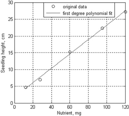
For example, the height of five seedlings and the amount of nutrients for each of them are 4.7, 7, 15.2, 22.3 and 27.2 cm and 12, 28, 60, 95, 120 mg. For fitting these data by the first-degree polynomial (m = 1), and for generating the next curve and data plot, the following script file, named fitexample, can be created:
After typing and entering the file name in the Command Window, the following coefficients are displayed and the graph in Figure 4.8 is generated:
Many bio-applications require an exponential or a logarithmic fitting function:
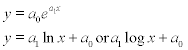
In the first case the fitting function should be rewritten as ln y = a1x + ln a0 and the polyfit function can be used with argument log(y) instead of y, e.g. a = polyfit(x, log(y),1) where in the vector a the a(1) element is a1 and a(2) is ln a0, thus a0 = exp(a(2)).
In the second case the polyfit function can be used with argument log(x) or log10(x) instead of x, e.g. a = polyfit(log(x), y,1) or a = polyfit(log10(x),y,1) where in vector a the a(1) element is a1 and a(2) is a0.
4.4 Application examples
4.4.1 Body mass index
Body mass index (BMI) I is a measure that relates the body weight G in kg and height h in m; it is defined as
This index is frequently used to assess how much an individual’s body weight departs from what is normal or desirable. A BMI between 20 and 25 kg/m2 is normal, below 20 underweight, between 25 and 30 overweight, and above 30 obese.
Problem: Compose a script program that calculates and displays the BMI of the user and writes a conclusion about the user’s weight.
In the script presented below, the user enters his/her weight and height, and the program then calculates the BMI, determines the user’s category and displays the results.
w = input('Enter your weight in kg'),
h = input('Enter your height in m'),
fprintf(' Your BMI is %5.1f kg/m^2, thus your weight is %s ',I,S)
With the script file name BMI entered into the Command Window, the program displays the prompt to input the weight in kg; with the weight typed and the Enter key pressed, a new prompt for height in m appears; with the latter typed and entered, the BMI is calculated and displayed together with a conclusion.
The following shows the Command Window when the file was run:
4.4.2 Basal metabolic rate
The basal metabolic rate (BMR) P in kcal/day is the human minimal daily energy requirement (in calories). For women this index is given by the expression:
where w is weight in kg, h is height in cm and a is age in years.
Problem: Write a script program for calculating and displaying the BMR. The script file solving this problem is written below.
sex = input('Enter the sex: 1 - male, 2 - female'),
w = input('Enter your weight in kg'),
h = input('Enter your height in m '),
a = input('Enter your age in years '),
P = 655 + 9.6*w + 1.8*h-4.7*a;
fprintf(' Your BMR is %5.1f cal/day ',P)
After entering into the Command Window the script file name BMR, the program displays the prompt to sex, type 1 or 2 (male or female). After pressing the enter key, prompts then appear successively about weight in kg, height in m and finally age. The BMR is then calculated and displayed.
The following shows the Command Window when the file was run:
4.4.3 Conversion of concentration units
The concentration of components in solutions is expressed in different forms, among them molarity, molality and molar fraction. Molarity M is the solute amount per liter of solution, mol/L; molality m is the solute amount per solvent mass, mol/kg; and molar fraction χ is the mole solute to mole solution ratio. The expression for conversion from M to m and to x is
where d is the solution density (g/L), M1 the molecular weight of the solute (g/mol) and M2 = 18 g/mol is the molecular weight of water.
Problem: Write a function file with name molfrac that calculates and displays solute molality and molar fraction for a given solute molarity and molar mass, and solution density. Calculate the molality and the molar fraction for these data: M = 3 mol/L, d = 1.5 × 10³ g/L and M1 = 40 g/mol (sodium hydroxide).
The input parameters in the function definition line are: solution density d, solute molarity M and molar mass of the solute M1; the output parameters are molality and molar_fraction. The function file is:
function [molality,molar_fraction] = molfrac(d,M,M1)
% molality (mol/l) and molar fraction calculations
% d is solution density in g/l
% M1 is solute molar mass in g/mol
The following shows the Command window when the file was run:
4.4.4 Population of Europe
Population statistics for Europe are:
![]()
Problem: Write a function file with name europes that predicts and displays the population in 2011. Use for prediction the interp1 function with three extrapolation alternatives provided: 1, linear; 2, cubic; 3, spline.
The first line of the function should be the function definition line with the function name europes and the input and output parameters. Thus, the following input parameters are specified: yi, the target year, and num, the chosen method alternative: 1, linear; 2, cubic; 3, any other number (except 1 and 2) for the spline. The specified output parameter is pei – the predicted population.
The function file written to solve the problem is:
function pei = europes(yi,num)
% Europe population prediction
% num - mehod number: 1-linear,2-cubic, 3-spline
p = [163 203 276 408 547 729 732];
pei = interp1(y,p,yi,method, 'extrap'),
The following appears in the Command Window when the file was run:
4.4.5 Reactant breakdown
In the two-stage consecutive reaction A → B → C, the concentration of intermediate reactant B can be expressed as
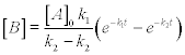
where [A]0 is the initial concentration of reactant A, k1 and k2 are the reaction rate constants for the A → B and B → C reactions, respectively, and t is time.
Problem: Write a function file reactime.m that evaluates and displays time t in the course of which the intermediate reactant B appears, accumulates and breaks down to the current concentration. Calculate the time for: [B] = 0.01 mol/L at initial concentration [A]0 = 2.5 mol/L, and constants k1 = 2.6 × 10⁻³ s−1 and k2 = 9.5 × 10⁻³ s−1; use for solution the fzero function with initial (guess) value x0 = 2 s.
The input parameters for the function definition line are: the concentrations [B] and [A]0, the reaction rate constants k1 and k2, and the initial value x0; the output parameter is time t. In using fzero, the variable t in the expression above should be named x. The function file for solving this problem is:
function t = reactime(A0,B,k1,k2,x0)
% time of reactant breakdown, t
% Ao is initial concentration of the reactant A, mol/l
% B is the intermediate component concentration, mol/l
% k1 is reaction rate constant of the A-to-B reaction
% k2 is reaction rate constant of the B-to-C reaction
t = fzero(@(x) reaction(x,A0,B,k1,k2),x0);
The following appears in the Command Window when the file was run:
4.4.6 Amount of compound
The decay rate v of a compound is given by v(t) = − 0.69*e−2.3t, where t is time in h, and v is in mol/h. The amount m of the compound after time t is:
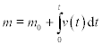
where m0 = 0.3 mol is the initial mass of the compound.
Problem: Write a script that calculates the amount of the compound every 30 minutes over 3 hours and plot the graph m(t).
The solution is organized in the following steps:
• define the variables m0 and t;
• organize a loop with for … end command for the amount of compound, m, calculated at different upper limits; for integration the quad function is used, in which the upper integration limit repeatedly changes from 0.5 up to 3 at steps of 0.5 hours;
The script to solve this problem is:
| % Amount of compound | |
| clear, close all | % clear the memory and close all preceding |
| % graphs | |
| m0 = 0.3 | % initial amount of compound |
| t = 0.5:0.5:3; | % times for upper integration limit |
| for i = 1:length(t) | % the loop for integration by the quard |
| % command |
q(i) = m0 + quad('-0.69*exp(− 2.3*t)',0,t(i));
fprintf(' Compound amount change Hour Mole ')
| % title for resulting table | |
| fprintf('%5.1f %8.5f ',[t;q]) | % displays resulting table |
| plot(t,q, '-o') | % plot the graph |
| title('Compound decay') | |
| xlabel('Time, h'),ylabel('Mass,mol') | |
| grid |
122This script was named and saved into the Integr2_Ex.m file. The following appears in the Command Window when the file was run:
| Hour | Mole |
| 0.5 | 0.09499 |
| 1.0 | 0.03008 |
| 1.5 | 0.00952 |
| 2.0 | 0.00302 |
| 2.5 | 0.00095 |
| 3.0 | 0.00030 |
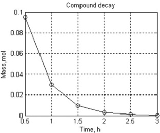
4.4.7 Dissociation rate
Species dissociation is described by the equation
where m0 and m are the amounts of the species initially and at time t, respectively, and k is the dissociation constant.
Problem: Write and save a function that calculates the reaction rate r = − dm/dt at t = 0, 0.1, …, 10 min, k = 1.8 min−1 and m0 = 5 mg, and plots the m(t) and r(t) curves in one graph.
The program is realized in the form of a function named DissRate with the following input arguments: m0, the species amount at starting time; k, the reaction constant; tstart, the starting time; tend, the end time; and h, the time step.
The solution is carried out in the following steps:
• the species amount vector m is calculated for the whole time interval – from tstart to tend with step h;
• the reaction rates are calculated as the –diff(m) to h ratio and assigned to the vector r;
• the resulting matrix is constructed, in which the first column is t and the second is r; the columns are adjusted to the same length, as r is one element shorter than t;
• the results are printed with the disp command;
• the m(t) function and its derivative are generated with the plot command and then the commands for axis and plot captions are added; the vector r is one element shorter than the t and m vectors, and thus the axis command is introduced to show both m(t) and dm/dt curves in the same t interval.
The function file to solve this problem is:
function DissRate(m0,k,tstart,tend,h)
% m0 is initial species amount, mg
% k is dissociation constant, 1/min
% tstart and tend are started and final values of time, min
plot(t,m,t_r(:,1),t_r(:,2),'-- ')
xlabel('time'),ylabel('m and dm/dt'),grid
legend('Function m(t)','Dissociation Rate dm/dt')
After running this file, the following appear in the Command and Figure windows:
| t | r |
| 0.1000 | 8.2365 |
| 0.2000 | 6.8797 |
| 0.3000 | 5.7464 |
| 0.4000 | 4.7998 |
| 0.5000 | 4.0091 |
| 0.6000 | 3.3487 |
| 0.7000 | 2.7971 |
| 0.8000 | 2.3363 |
| 0.9000 | 1.9515 |
| 1.0000 | 1.6300 |
| 1.1000 | 1.3615 |
| 1.2000 | 1.1372 |
| 1.3000 | 0.9499 |
| 1.4000 | 0.7934 |
| 1.5000 | 0.6627 |
| 1.6000 | 0.5535 |
| 1.7000 | 0.4624 |
| 1.8000 | 0.3862 |
| 1.9000 | 0.3226 |
| 2.0000 | 0.2694 |
4.4.8 Fitting of cancer incidence data
A high level of a particular substance in the atmosphere may increase the incidence of cancer. Assume that the function that relates cancer incidence Y to the amount of carcinogen X is polynomial. Observed cancer incidences are 10, 10, 30, 35, 55 and 120 at carcinogen concentrations respectively of 10, 40, 100, 200, 300 and 400 (dimensionless).
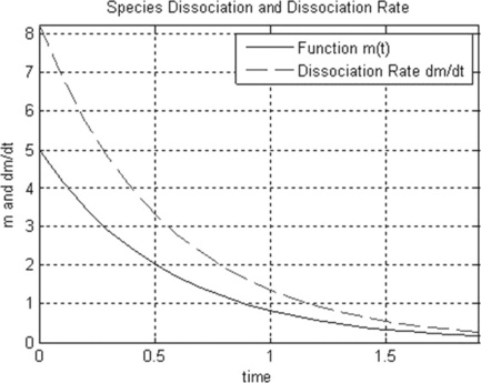
Problem: Write and save a function that requires degree of polynomial as input parameter, and then fits the cancer incidence–carcinogen concentration data, displays fitting coefficients and plots y(x) points with defined polynomial curve. Take the degree of polynomial to be no more than 5.
disp('Error: Polynomial degree can not be more than 5')
y = [10, 10, 20, 35, 55, 120];
disp('Polynomial coefficients are:'),disp(a')
disp('Polynomial degree is:'),disp(m)
x_pol = linspace(min(x),max(x),10);
xlabel('Concentration of substance'),ylabel('Cancer incidence')
This function file with this function has the name cancer. For running, the function requires the value of polynomial degree, m. The first line of cancer represents the definition of the function and the next three lines represent function help. After running, the function determines the fitting coefficients with the polyfit command, displays the latter and the polynomial degree with the disp commands, and plots the fit results together with the original data. If the inputted degree is more than 5 (the number of coefficients in the polynomial is m + 1 and it cannot be more than the number of points), the program displays ‘Error: Polynomial degree cannot be more than 5’, and the run should be repeated with the correct m value.
The Command Window and generated plot for polynomial degree 3 are:
4.5 Questions for self-checking and exercises
1. The user-defined MATLAB® function has in the first line: (a) the function definition; (b) help comments; or (c) definition of global variables?
2. Local variables are: (a) all variables defined, recognized and used only within the function file; (b) input/output parameters only, written in the function definition line; or (c) the variables appearing in the workspace after the function file has completed its work?
3. The unterp1 function is used: (a) for interpolation only; (b) for extrapolation only; or (c) for both interpolation and extrapolation?
4. In which form should the equation ae−kx = b be written for solution with the aid of the fzero function: (a) just as it is written: b = ae−kx; (b) ae−kx – b = 0; or (c) ln(b/a) = − kx?
5. The function f(x) is given by data points; which MATLAB® function should be used for its integration: (a) quad, (b) trapz or (c) fzero?
is used to convert degrees Fahrenheit F into degrees Centigrade C. Write the script that can be used as a Fahrenheit to Centigrade converter; display the result to two decimal places.
7. The death time t of spores in a thermal sterilization process is described by the equation
where T is temperature in degrees Celcius, and t is time in seconds. Write the script that calculates and displays the death time of the spores at 100, 110, …, 180 °C. Plot the graph T as function of t, and add axis labels, grid and captions to the graph.
8. The van der Waals gas equation of state is:
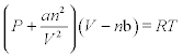
where P is pressure in atmospheres, V is volume in liters, T temperature in Kelvin, n is the number of moles, and a and b are constants that should be specified for each gas. Write the function file that calculates the volume of the gas at given P, T, n, a and b; use the fzero function to obtain V at P = 6 atm, T = 50 °C (323.15 K), n = 2 mol, R = 0.08206 L-atm/mol-K, a = 5.43 L2atm/mol2, b = 0.0304 L/mol (water) and initial V = 5.
9. The waist-to-hip ratio (WHR) R = waist/hip is used as an indicator or measure of the state of health of a person; when this ratio is in the range 0.7–0.85 for women and 0.76–0.9 for men, it is ranked as normal; persons with higher WHRs (‘apple-shaped’ body) face a higher health risk than those with lower WHRs (‘pear-shaped’ body). Write a function file with waist and hip as input parameters, and R and information about the person’s state of health (normal, high health risk, low health risk) as output parameters.
10. New York city population between 1900 and 2000:
![]()
Write a user-defined function with the table data, and enter into it the interp1 command with the 'linear' method to calculate the population within and outside the table range; save the defined function in the function file and use it to calculate the population in 1899, 2010 and 2012.
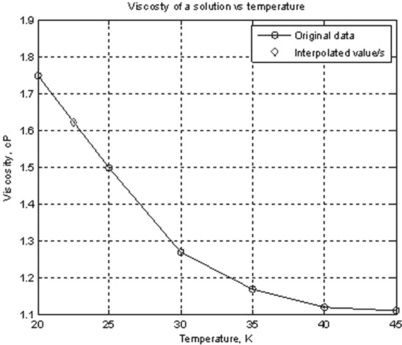
11. The viscosity of a solution η is 1.75, 1.5, 1.27, 1.3, 1.15 and 1.1 cP at temperatures t of 20, 25, 30, 35, 40 and 45 °C, respectively. Write a user-defined function that describes the graph η(t) together with interpolated values, and add to the graph axis labels, grid, legend and a caption; use the interp1 command with the ‘cubic’ method to obtain the viscosity at temperatures within the above range; save the function into a function file and use it to obtain the viscosity at 22.5 °C.
12. The integral of a function f(x) can be calculated by the left Riemann sum equation:
where n is the number of points in the integration interval [a,b], Δx = (b – a)/(n – 1) is the spacing of the points, and fi is the value of the function at point i = 1, 2, …, n – 1. Calculate by this the bacterial population

where time t is in hours, the proliferation rate v(t) = 0.6931.N0.2t, the initial bacterial amount N0 = 10 cells, and the integration limits are a = 0 and b = 7 hours. Write and save the program as a function file with input parameters a, b, n, N0 and output parameter N; run it with n = 1000. The resulting N should be given rounded to the nearest integer value.
13. Solve the integral in exercise 12 by the right Riemann sum equation:
where Δx and fi have the same sense as in exercise 12. Write and save the program as a function file; run it with n = 100, 500 and 1000. Use the function written in exercise 12 to display the results obtained for the left and right Riemann methods. Note: the input and output parameters of the function created should be suitable to solve the problem.
14. Solve the integral in exercise 12 with the quad command. Write and save the program as a function file. Use the functions written in exercises 12 and 13 to display the results obtained with the quad command and with the left and right Riemann methods (for n = 1000). Note: the input and output parameters of the function created should be suitable to solve the problem.
15. Bacterial population growth is expressed by the polynomial p = 106 + 104 t – 103 t2, where t is time in hours. Write the script that determines numerically the bacterial growth rate r = dp/dt when t = 1 hour. Take a time step equal to 0.01 hour and count the derivatives one step longer than the required t.
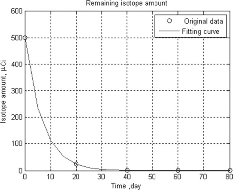
16. The decay rate of a certain radioisotope is described by the equation m = m0e−kt where t is time, m and m0 are the isotope amounts at the starting and current time, respectively, and k is the decay constant. Values of m of 500, 250, 125, 63 and 31 μCi were measured on days 0, 20, 40, 60 and 80, respectively. Write a function without parameters that fits these data by the above equation, displays the fitting equation with the found coefficients m0 and k, and plots the fitting curve and original data.
4.6 Answers to selected exercises
2. (b) Input/output parameters, only written in the function definition line.
6. Enter temperature as Fahrenheit 82
Temperature 82.00 degrees Fahrenheit is 27.78 degrees Celsius
1The symbol @ is used in MATLAB to denote the so-called anonymous functions, which fall outside the scope of this book.