Chapter 5 – Tera-Tom’s Top Tips
“Let me once again explain the rules. Tera-Tom Rules!”
-Tera-Tom fan
Tera-Tom's Top Tips
1. When given a choice between using a join or a subquery, use
the join.
2. Change your expression's subselects by moving the subselect from the WHERE clause to the FROM clause or by rewriting it as a join.
3. Use an inner subquery to shrink the size of data on which outer queries needs to operate. Likewise, use an inner subquery to shrink the size of a relation before the data is redistributed on a different distribution key.
4. Avoid per-row functions or delay them. Group rows first, and then apply the function.
5. Avoid doing JOINs, GROUP BYs, and WHERE clauses on data types that are non-native.
6. EXPLAIN should be used before any new query.
Above are tips for your consideration. The larger the data, the more you will need them.
Tera-Tom's Top Tips # 2
2. Change your expression's subselects by moving the subselect from the WHERE clause to the FROM clause or by rewriting it as a join.
Subquery here:
SELECT * FROM Customer_Table
WHERE Customer_Number IN
(SELECT Customer_Number FROM Order_Table
WHERE Order_Date IS NOT NULL) ;
Rewritten as a join
SELECT C.* FROM Customer_Table as C,
Order_Table as O
WHERE C.Customer_Number = O.Customer_Number AND Order_Date IS NOT NULL ;
Above are tips for your consideration. The larger the data the more you will need them.
Tera-Tom's Top Tips #3
3. Use an inner subquery to shrink the size of data on which outer queries needs to operate. Likewise, use an inner subquery to shrink the size of a relation before the data is redistributed on a different distribution key.
SELECT inv.product_id,
SUM(s.sales_quantity * (inv.unit_list_price - inv.cost) - s.discount_amount)
AS total_profit
FROM Sales_Table AS s,
Inventory_Table as inv
WHERE s.product_id = inv.product_id
AND s.sales_date > '01-Jan-2013'
GROUP BY inv.product_id;
This query will be rewritten
Above are tips for your consideration. The larger the data the more you will need them.
Tera-Tom's Top Tips # 3 Rewritten
SELECT inv.product_id,
SUM(t.total_sold * (inv.unit_list_price - inv.cost) - t.total_product_discount)
AS Total_Profit
FROM
(
SELECT s.product_id as product_id,
SUM(s.sales_quantity) AS total_sold,
SUM(s.discount_amount) AS total_product_discount
FROM Sales_Table as S
WHERE s.sales_date > '01-Jan-2013'
GROUP BY s.product_id
) AS t,
Inventory_Table as inv
WHERE t.product_id = inv.product_id
GROUP BY inv.product_id;
In the rewritten query above, the GROUP BY is designed to speed up the query. Now, the grouping of rows is performed in a distributed fashion on the vworkers before the product_id values (only) are passed to the queen for filtering of the distinct values.
Tera-Tom's Top Tips #4
4. Avoid per-row functions or delay them. Group rows first, and then apply the function.
CREATE FACT TABLE Orders (
Order_ID int PRIMARY KEY,
Customer_ID int NOT NULL,
Amount int,
Order_Date date )
DISTRIBUTE BY HASH (Customer_ID);
SELECT Customer_ID, COUNT(*)
FROM Orders GROUP BY Customer_ID ;
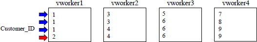
The Customer_ID's in each Grouping are on the same vworker.
Aster performs GROUP BYs at lightning speed when the distribution key is used as the GROUP BY column. This includes when the distribution key is in the list of GROUP BY values. This is because all like values in a group need to be on the same vworker to be calculated, and if the GROUP BY column is the distribution key, then all like values are on the same vworker. This is why the GROUP BY is so fast. This is what is called "Local" processing.
When the GROUP BY Column is NOT the Distribution Key
CREATE FACT TABLE Orders (
Order_ID int PRIMARY KEY,
Customer_ID int NOT NULL,
Amount int,
Order_Date date )
DISTRIBUTE BY HASH (Order_ID);
SELECT Customer_ID, COUNT(*)
FROM Orders
GROUP BY Customer_ID
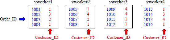
The Table is Hashed on Order_ID, but the query is Grouped by Customer_ID.
Aster performs GROUP BYs at lightning speed when the distribution key is used as the Group By column, but watch what happens when the GROUP BY is performed on a column that is NOT the Distribution Key.
Example of GROUP BY Column is NOT the Distribution Key
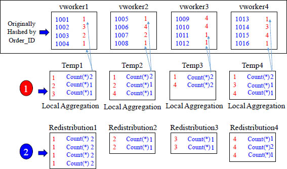
Step 1 involves local aggregation in a temp table to count the Customer_ID's within each vworker. Then, in step 2, the actual Customer_ID is hashed and transferred over the network in a redistribution. Then, because of the hash, all like Customer_ID's landed together on a vworker. There they could once again locally be counted and sent to the queen. You can see this is a smart way to do this because it minimizes network traffic by pre-aggregating locally.
Tera-Tom's Top Tips #5
5. Avoid doing JOINs, GROUP BYs, and WHERE clauses on non-native data types. For example, avoid numeric, varchar, char arrays. These are non-native data types. You should use integers, floats, doubles, and char because these are native data types. These can then be converted to non-native data types after the JOIN, GROUP BY, and WHERE have taken place.
CREATE FACT TABLE Bad_Example (
Order_ID int,
Customer_ID varchar,
Amount int,
Order_Date date )
DISTRIBUTE BY HASH (Customer_ID);
SELECT B.*, C.*
FROM Customer_Table as C,
Bad_Example as B
WHERE C.Customer_Number = B.Customer_ID;
Nothing is worse than good advice . . . that you just didn't take. Know your data types.
Tera-Tom's Top Tips #6 – Use EXPLAIN
Here are some of the key terms in the Aster EXPLAIN Function:
Number: Each high level phase gets a number.
Statement: The statement that is executed by the vworkers.
Result Table: The output that will be used later is placed in this table.
Operation Type: The operation being performed. This could be Pre-condition, Statement Execution, Repartition Tuples (rows), Broadcast Tuples (copy to all vworkers).
Location: Where the phase is being executed. This will most likely be workers (all workers), but could be Queen or AnyWorker (single worker).
Query Plan and Estimates: vworker-level query plan and cost estimates. Costs are relative, and it is assumed that the fetching of 8KB of sequential data from disk is a decimal value of 1 unit of work.
Data Size Distribution: This gives an estimate of the mean and standard deviation of data coming in from worker nodes in bytes. This is only for queries that require transfer of data to queen or worker.
The EXPLAIN command displays the execution plan that the Queen uses for the query, and cost estimates for each of the steps of the Queen's plan. The plan displays information on the exact SQL statements executed in order to satisfy the query, including whether network transfers of data are required and for what purpose. The plan also provides the location at which each step is executed, and the low-level algorithms used to execute a step at the slowest node. The EXPLAIN itself does not execute the statement, but merely shows the plan. It is a good idea to look at the explain in any development environment.
Query Plan and Estimates
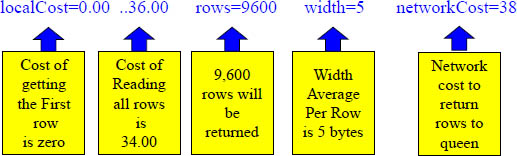
Query Plan and Estimates: vworker-level query plan and cost estimates. Costs are relative, and it is assumed that the fetching of 8KB of sequential data from disk is a decimal value of 1 unit of work. The cost of transferring 1 KB of network data is set to 1. The first line of the output displays the summary of the entire query. Below is an example and explanation of what each value means.
The above costs are from Phase one. From the second line onward, the output is from where the query is going to be executed (the Node). If the query will run on multiple workers, then statistics are displayed from the slowest worker. It is here where you can see which scan, sort, or join algorithms will be applied at the node level.
Explain Plan Showing a Hash Join
EXPLAIN SELECT E.*, D.Department_Name
FROM Employee_Table AS E
INNER JOIN
Department_Table AS D
ON E.Dept_No = D.Dept_No ;
QUERY PLAN
Hash Join (cost=1.02..2.26 rows = 7 width = 70)
Hash Cond: (E.Dept_No = D.Dept_No)
-- > SeqScan on Employee_Table (cost=0.00..1.10 rows=7 width=75)
-- > Hash (cost=1.01..1.01 rows=4 width=24)
-- > SeqScan on Department_Table (cost=0.00..1.01 rows=4 width=45)
The above explain is from the worker and describes a Hash Join. A Hash Join takes the smaller table, collects the distinct values from its join column, and places its contents in memory. This will be the fastest join and happens when one of the tables is small enough to fit in memory.
Explain Plan Showing a Merge Join
EXPLAIN SELECT O.*, Customer_Name
FROM Order_Table AS O
INNER JOIN
Customer_Table AS C
ON O.Customer_Number = C.Customer_Number;
QUERY PLAN
Merge Join (cost=56070.12..67288.26 rows = 350045 width = 150)
Merge Cond: (Employee_Table.Dept_No = Department_Table.Dept_No)
-- > Index Scan using Order_Number O (cost=0.00..3556.10 rows=100000 width=73)
-- > Materialize (cost=56789.01..59675.01 rows=312351 width=24)
-- > Sort (cost=58768.10..58798.01 rows=312351 width=70)
Sort Key: Customer_Table.Customer_Number
-- > SeqScan on Customer_Table (cost=0.00..6743.22 rows=312351 width=70)
The above explain is from the worker and describes a Merge Join. The merge join above sorts both tables on the column Customer_Number and then streams the top few rows from each table to do the join. This makes for a very low memory utilization during the join operation. The sorting step requires memory and is the most memory intrusive.
Explain Plan Showing a Nested Loop Join
EXPLAIN SELECT O.*, Item_Description
FROM Order_Table AS O
INNER JOIN
Item_Table AS I
ON I.Order_Number = O.Order_Number
WHERE O.Order_Number = 123456 ;
QUERY PLAN
Nested Loop (cost=0.00..7288.26 rows = 100 width = 140)
-- > Index Scan using O.Order_Number (cost=0.00..7099.10 rows=1002 width=71)
Index Cond: (O.Order_Number=123456)
-- > Index Scan on Item_Table.pk_itemon(cost=0.00..7909.01 rows=100 width=72)
Index Cond: (Order_Table.Order_Number=Item_Table.Order_Number)
The above example describes Nested Loop Join. The Nested Loop joins are fast to produce the first record and will be used if the optimizer thinks both of the tables are small. The Nested Loop Join also works well if one of the tables is really small and the larger table has an index on the joining column. It is important to run ANALYZE so the optimizer knows its options.