3

Domain Partitioning

The purpose of this chapter is to introduce techniques for the generation of test data from informally and formally specified requirements. Essentially, conditions in the form of predicates are extracted either from the informally or formally specified requirements or directly from the program under test. There exists a variety of techniques to use one or more predicates as input and generate tests. Some of these techniques can be automated while others may require significant manual effort for large applications. It is not possible to categorize the techniques in this chapter as either black- or white-box technique. Depending on how tests are generated, a technique could be termed as a black- or white-box technique.

3.1  Introduction

Requirements serve as the starting point for the generation of tests. During the initial phases of development, requirements may exist only in the minds of one or more people. These requirements, more aptly ideas, are then specified rigorously using modeling elements such as use cases, sequence diagrams, and statecharts in UML. Rigorously specified requirements are often transformed into formal requirements using requirements specification languages such as Z, S, and RSML.

 

While a complete formal specification is a useful document, it is often the case that aspects of requirements are captured using appropriate modeling formalisms. For example, Petri nets and its variants are used for specifying timing and concurrency properties in a distributed system, timed input automata to specify timing constraints in a real-time system, and finite state machines to capture state transitions in a protocol. UML is an interesting formalism in that it combines into a single framework several different notations used for rigorously and formally specifying requirements.

A requirement specification can thus be informal, rigorous, formal, or a mix of these three approaches. Usually, requirements of commercial applications are specified using a mix of the three approaches. In either case, it is the task of the tester, or a test team, to generate tests for the entire application regardless of the formalism in which the specifications are available. The more formal the specification, the higher are the chances of automating the test generation process. For example, specifications using finite state machines, timed automata, and Petri nets can be the inputs to a programmed test generator and tests generated automatically. However, significant manual effort is required when generating test cases from use cases.

Often, high-level designs are also considered as part of requirement specification. For example, high-level sequence and activity diagrams in UML are used for specifying interaction amongst high-level objects. Tests can also be generated from such high-level designs.

In this chapter, the focus is on the generation of tests from informal and rigorously specified requirements. These requirements serve as a source for the identification of the input domain of the application to be developed. A variety of test generation techniques are available to select a subset of the input domain to serve as test set against which the application will be tested.

Figure 3.1 lists the techniques described in this chapter. The figure shows requirements specification in three forms: informal, rigorous, and formal. The input domain is derived from the informal and rigorous specifications. The input domain then serves as a source for test selection. Various techniques, listed in the figure, are used to select a relatively small number of test cases from a usually large input domain.

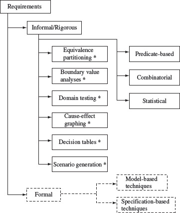
Figure 3.1 Techniques listed here, and marked with an asterisk, for test selection from informal and rigorously specified requirements, are introduced in this chapter. Techniques from formally specified requirements using graphical models and logic-based languages are discussed in other chapters.

The remainder of this chapter describes each of the techniques marked in the figure. All techniques described here fall under the “black-box” testing category. However, some could be enhanced if the program code is available. Such enhancements are discussed in Part III of this book.

 

3.2  The Test Selection Problem

Let D denote the input domain of program p. The test selection problem is to select a subset T of tests such that execution of p against each element of T will reveal all errors in p. In general there does not exist any algorithm to construct such a test set. However, there are heuristics and model-based methods that can be used to generate tests that will reveal certain types of faults. The challenge is to construct a test set T ⊆ D that will reveal as many errors in p as possible. As discussed next, the problem of test selection is difficult due primarily to the size and complexity of the input domain of p.

 

An input domain for a program is the set of all possible legal inputs that the program may receive during execution. The set of legal inputs is derived from the requirements. In most practical problems, the input domain is large, i.e. has many elements, and often complex, i.e. the elements are of different types such as integers, strings, reals, Boolean, and structures.

The large size of the input domain prevents a tester from exhaustively testing the program under test against all possible inputs. By “exhaustive” testing, we mean testing the given program against every element in its input domain. The complexity makes it harder to select individual tests. The following two examples illustrate what causes large and complex input domains.

 

Example 3.1   Consider program Ρ that is required to sort a sequence of integers into ascending order. Assuming that Ρ will be executed on a machine in which integers range from –32768 to 32767, the input domain of Ρ consists of all possible sequences of integers in the range [–32768, 32767].

If there is no limit on the size of the sequence that can be an input, then the input domain of Ρ is infinitely large and Ρ can never be tested exhaustively. If the size of the input sequence is limited to, say, Ν > 1, then the size of the input domain depends on the value of N. In general, denoting the size of the input domain by S, we get

where v is the number of possible values each element of the input sequence may assume, which is 65536. Using the formula given above, it is easy to verify that the size of the input domain for this simple sort program is enormously large even for small values of N. Even for small values of N, say N = 3, the size of the input space is large enough to prevent exhaustive testing.

 

Example 3.2   Consider a procedure Ρ in a payroll processing system that takes an employee record as input and computes the weekly salary. For simplicity, assume that the employee record consists of the following items with their respective types and constraints:

 

ID: int;	ID is 3-digits long from 001 to 999.
name: string;	name is 20 characters long; each character belongs to the set of 26 letters and a space character.
rate: float;	rate varies from $5 to $10 per hour; rates are in multiples of a quarter.
hoursWorked: int;	hoursWorked varies from 0 to 60.

 

Each element of the input domain of Ρ is a structure that consists of four items listed above. This domain is large as well as complex. Given that there are 999 possible values of ID, 27²⁰ possible character strings representing names, 21 hourly pay rates, and 61 possible work hours, the number of possible records is

 

999 × 27²⁰ × 21 × 61 ≈ 5.42 × 10³⁴.

 

Once again, we have a huge input domain that prevents exhaustive testing. Notice that the input domain is large primarily due to the large number of possible names that represent strings and the combinations of the values of different fields.

For most useful software, the input domains are even larger than the ones in the above examples. Further, in several cases, it is often difficult to even characterize the complete input domain due to relationships between the inputs and timing constraints. Thus, there is a need to use methods that will allow a tester to be able to select a much smaller subset of the input domain for the purpose of testing a given program. Of course, as we will learn in this book, each test selection method has its strengths and weaknesses.

3.3  Equivalence Partitioning

Test selection using equivalence partitioning allows a tester to subdivide the input domain into a relatively small number of subdomains, say Ν > 1, as shown in Figure 3.2(a). In strict mathematical terms, the subdomains by definition are disjoint. The four subsets shown in Figure 3.2(a) constitute a partition of the input domain while the subsets in Figure 3.2(b) are not. Each subset is known as an equivalence class.

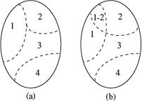
Figure 3.2 Four equivalence classes created from an input domain. (a) Equivalence classes together constitute a partition as they are disjoint. (b) Equivalence classes are not disjoint and do not form a partition. 1-2 indicates the region where subsets 1 and 2 overlap. This region contains test inputs that belong to subsets 1 and 2.

The equivalence classes are created assuming that the program under test exhibits the same behavior on all elements, i.e. tests, within a class. This assumption allows a tester to select exactly one test from each equivalence class resulting in a test suite of exactly Ν tests.

 

Of course, there are many ways to partition an input domain into equivalence classes. Hence, the set of tests generated using the equivalence partitioning technique is not unique. Even when the equivalence classes, created by two testers, are identical, the testers might select different tests. The fault detection effectiveness of the tests so derived depends on the tester’s experience in test generation, familiarity with the requirements, and when the code is available, familiarity with the code itself. In most situations, equivalence partitioning is used as one of the several test generation techniques.

3.3.1  Faults targeted

The entire set of inputs to any application can be divided into at subsets: one containing all expected (E), or legal, inputs and the other containing all unexpected (U), or illegal, inputs. Each of the two subsets, E and U, can be further subdivided into subsets on which the application is required to behave differently. Equivalence class partitioning selects tests that target any faults in the application that cause it to behave incorrectly when the input is in either of the two classes or their subsets. Figure 3.3 shows a sample subdivision of all possible inputs to an application.

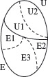
Figure 3.3 Set of inputs partitioned into two regions one containing expected (E), or legal, and the other containing unexpected (U), or illegal, inputs. Regions Ε and U are further subdivided based on the expected behavior of the application under test. Representative tests, one from each region, is targeted at exposing faults that cause the application to behave incorrectly in their respective regions.

For example, consider an application A that takes an integer denoted by age as input. Let us suppose that the only legal values of age are in the range [1, 120]. This set of input values is now divided into a set Ε containing all integers in the range [1, 120] and a set U containing the remaining integers.

Furthermore, assume that the application is required to process all values in the range [1, 61] in accordance with requirement R₁ and those in the range [62, 120] according to requirement R₂. Thus, Ε is further subdivided into two regions depending on the expected behavior. Similarly, it is expected that all invalid inputs less than 1 are to be treated in one way while all greater than 120 are to be treated differently. This leads to a subdivision of U into two categories.

 

Tests selected using the equivalence partitioning technique aim at targeting faults in A with respect to inputs in any of the four regions, i.e. two regions containing expected inputs and two regions containing the unexpected inputs. It is expected that any single test selected from the range [1, 61] will reveal any fault with respect to R₁. Similarly, any test selected from the region [62, 120] will reveal any fault with respect to R₂. A similar expectation applies to the two regions containing the unexpected inputs.

The effectiveness of tests generated using equivalence partitioning for testing application A is judged by the ratio of the number of faults these tests are able to expose to the total faults lurking in A. As is the case with any test selection technique in software testing, the effectiveness of tests selected using equivalence partitioning is less than 1 for most practical applications. However, the effectiveness can be improved through an unambiguous and complete specification of the requirements and carefully selected tests using the equivalence partitioning technique described in the following sections.

3.3.2  Relations

Recalling from our knowledge of sets, a relation is a set of n-ary tuples. For example, a method addList that returns the sum of elements in a list of integers defines a binary relation. Each pair in this relation consists of a list and an integer that denotes the sum of all elements in the list. Sample pairs in this relation include ((1, 5), 6) and ((–3, 14, 3), 14), and (( ), 0). Formally, the relation computed by addList is defined as follows.

 

 

where L is the set of all lists of integers and ℤ denotes the set of integers. Taking the example from the above paragraph as a clue, we can argue that every program, or method, defines a relation. Indeed, this is true provided the domain, i.e. the input set, and the range, i.e. the output set, are defined properly.

 

For example, suppose that the addList method has an error due to which it crashes when supplied with an empty list. In this case, even though addList is required to compute the relation defined in the above paragraph, it does not do so due to the error. However, it does compute the following relation:

 

 

Relations that help a tester partition the input domain of a program are usually of the kind

 

 

where I denotes the input domain. Relation R is on the input domain. It defines an equivalence class that is a subset of I. The following examples illustrate several ways of defining R on the input domain.

 

Example 3.3   Consider a method gPrice that takes the name of a grocery item as input, consults a database of prices, and returns the unit price of this item. If the item is not found in the database, it returns with a message Price information not available.

The input domain of gPrice consists of names of grocery items which are of type string. Milk, Tomato, Yogurt, and Cauliflower are sample elements of the input domain. Obviously, there are many others. For this example, we assume that the price database is accessed through another method and hence is not included in the input domain of gPrice. We now define the following relation on the input domain of gPrice.

 

pFound : I→I

 

The pFound relation associates elements t₁ and t₂ if gPrice returns a unit price for each of these two inputs. It also associates t₃ and t₄ if gPrice returns an error message on each of the two inputs. Now suppose that the price database is as in the following table.

Item	Unit Price
Milk	2.99
Tomato	0.99
Kellogg’s Cornflakes	3.99

The inputs Milk, Tomato, and Kellogg’s Cornflakes are related to each other through the relation pFound. For any of these inputs, gPrice is required to return the unit price. However, for input Cauliflower, and all other strings representing the name of a grocery item not on the list above, gPrice is required to return an error message. Arbitrarily constructed strings that do not name any grocery item belong to another equivalence class defined by pFound.

Any item that belongs to the database can be considered as a representative of the equivalence class. For example, Milk is a representative of one equivalence class denoted as [Milk] and [Cauliflower] is a representative of another equivalence class.

Relation pFound defines equivalence classes, say pF and pNF, respectively. Each of these classes is a subset of the input domain I of gPrice. Together, these equivalence classes form a partition of the input domain I because pF ∪ pNF = I and pF ∩ pNF = ∅.

In the previous example, the input assumes discrete values such as Milk and Tomato. Further, we assumed that gPrice behaves the same for all valid values of the input. There may be situations where the behavior of the method under test depends on the value of the input that could fall into any of several categories, most of them being valid. The next example shows how, in such cases, multiple relations can be defined to construct equivalence classes.

 

In several cases, multiple relations are useful in defining equivalence classes. Such cases arise when the program under test behaves differently for different classes of inputs.

Example 3.4   Consider an automatic printer testing application named pTest. The application takes the manufacturer and model of a printer as input and selects a test script from a list. The script is then executed to test the printer. Our goal is to test if the script selection part of the application is implemented correctly.

The input domain I of pTest consists of strings representing the printer manufacturer and model. If pTest allows textual input through keyboard, then strings that do not represent any printer recognizable by pTest also belong to I. However, if pTest provides a graphical user interface to select a printer, then I consists exactly of the strings offered in the pulldown menu.

The script selected depends on the type of the printer. For simplicity, we assume that the following three types are considered: color inkjet (ci), color laserjet (cl), and color multifunction (cm). Thus, for example, if the input to pTest is “HP Deskjet 6840” the script selected will be the one to test a color inkjet printer. The input domain of pTest consists of all possible strings, representing valid and invalid printer names. A valid printer name is one that exists in the database of printers used by pTest for the selection of scripts while an invalid printer name is a string that does not exist in the database.

For this example, we define the following four relations on the input domain. The first three relations below correspond to the three printer categories while the fourth relation corresponds to an invalid printer name.

 

ci : I → I

cl : I → I

cm : I → I

invP : I → I

 

Each of the four relations above defines an equivalence class. For example, relation cl places all color laserjet printers into one equivalence class and all other printers into another equivalence class. Thus, each of the four relations defines two equivalence classes for a total of eight equivalence classes. While each relation partitions the input domain of pTest into two equivalence classes, the eight classes overlap. Notice that relation invP might be empty if pTest offers a list of printers to select from.

We can simplify our task of partitioning the input domain by defining a single equivalence relation pCat that partitions the input domain of pTest into four equivalence classes corresponding to the categories ci, cl, cm, and invP.

 

In software testing, an equivalence partition is not always a true partition in a mathematical sense. This is because the equivalence classes may overlap.

The example above shows that equivalence classes may not always form a partition of the input domain due to overlap. The implication of such an overlap on test generation is illustrated in the next subsection.

The two examples above show how to define equivalence classes based on the knowledge of requirements. In some cases, the tester has access to both the program requirements and its code. The next example shows a few ways to define equivalence classes based on the knowledge of requirements and the program text. 

Example 3.5   The wordCount method takes a word w and a file name f as input and returns the number of occurrences of w in the text contained in the file named f. An exception is raised if there is no file with name f. Using the partitioning method described in the examples above, we obtain the following equivalence classes.

 

El: Consists of pairs (w, f) where w is a string and f denotes a file that exists.

E2: Consists of pairs (w, f) where w is a string and f denotes a file that does not exist.

 

Now suppose that the tester has access to the code for wordCount.

The partial pseudo code for wordCount is given below.

 

Program P3.1

1   begin

2     string w, f;

3     input (w, f);

4     if ( not exists(f)) {raise exception; return(0)};

5     if (length(w)==0)return(0);

6     if(empty(f)) return(0);

7     return(getCount(w, f));

8   end

 

The code above contains eight distinct paths created by the presence of the three if statements. However, as each if statement could terminate the program, there are only six feasible paths. We can define a relation named covers that partitions the input domain of wordCount into six equivalence classes depending on which of the six paths is covered by a test case. These six equivalence classes are defined in the following table.

 

All inputs that force a program to follow the same path, can be considered as constituting an equivalence class.

Equivalence class	w	f
E1	non-null	exists, non-empty
E2	non-null	does not exist
E3	non-null	exists, empty
E4	null	exists, non-empty
E5	null	does not exist
E6	null	exists, empty

We note that the number of equivalence classes without any knowledge of the program code is two, whereas the number of equivalence classes derived with the knowledge of partial code is 6. Of course, an experienced tester will likely derive the six equivalence classes given above, and perhaps more, even before the code is available (see Exercise 3.6).

In each of the examples above, we focused on the inputs to derive the equivalence relations and, hence, equivalence classes. In some cases, the equivalence classes are based on the output generated by the program. For example, suppose that a program outputs an integer. It is worth asking: “Does the program ever generate a 0? What are the maximum and minimum possible values of the output?” These two questions lead to the following equivalence classes based on outputs.

 

E1: Output value ν is 0.

E2: Output value ν is the maximum possible.

E3: Output value ν is the minimum possible.

E4: All other output values.

 

Based on the output equivalence classes, one may now derive equivalence classes for the inputs. Thus, each of the four classes given above might lead to one equivalence class consisting of inputs. Of course, one needs to carry out such output-based analysis only if there is sufficient reason to believe that it will likely generate equivalence classes in the input domain that cannot be generated by analyzing the inputs and program requirements.

3.3.3  Equivalence classes for variables

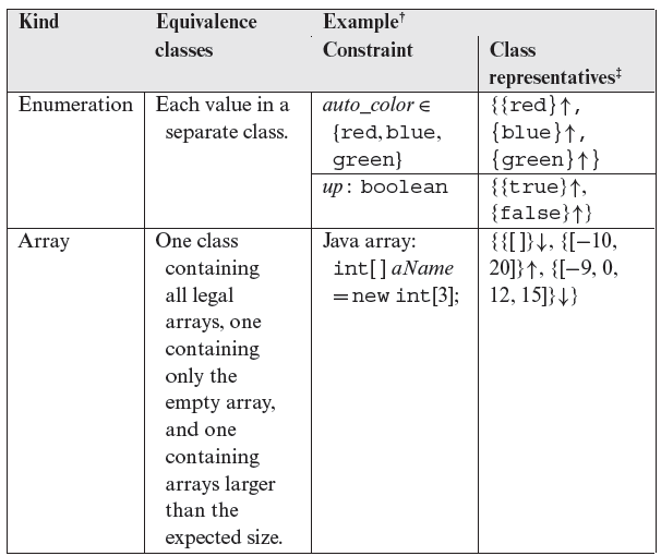
Tables 3.1 and 3.2 offer guidelines for partitioning variables into equivalence classes based on their type. The examples given in the tables are assumed to be derived from the application requirements. As explained in the following section, these guidelines are used while deriving equivalence classes from the input domain of an entire application that uses several input variables. Below we discuss the entries listed in Tables 3.1 and 3.2.

Range: A range may be specified implicitly or explicitly. For example, the value of speed is in the explicitly specified range [60, 90], whereas the range for the values of area is specified implicitly. In the former case, one can identify values outside of the range. In the case of area, even though it is possible to identify values outside of the range, it may be impossible to input these values to the application because of representational constraints imposed by the underlying hardware and software of the machine on which the application is being tested.

 

Table 3.1 Guidelines for generating equivalence classes for variables: range and strings.

 

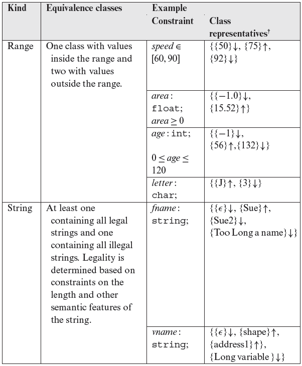
Table 3.2 Guidelines for generating equivalence classes for variables: enumeration and arrays.

 

The range for the values of age has also been specified implicitly. However, if, for example, age represents the age of an employee in a payroll processing application, then the tester must be able to identify the range of values from the knowledge of the semantics of age. In this case, age cannot be less than 0 and 120 is a reasonable upper limit. The equivalence classes for letter have been determined based on the assumption that letter must be one of 26 letters A through Z.

In some cases, an application might subdivide an input into multiple ranges. For example, in an application related to social security, age may be processed differently depending on which of the following four ranges it falls into: [1, 61], [62, 65], [67, 67], and [67, 120]. In this case, there is one equivalence class for each range and one each for a values less than the smallest value and larger than the highest value in any range. For this example, we obtain the following representatives from each of the six equivalence classes: 0 (↓), 34 (↑), 64 (↑), 67 (↑), 72 (↑), and 121 (↓). Further, if there is reason to believe that 66 is a special value and will be processed in some special way by the application, then 66 (↓) must be placed in a separate equivalence class, where, as before, ↓ and ↑ denote, respectively, values from equivalence classes containing illegal and legal inputs.

 

Strings: Semantic information has also been used in the table to partition values of fname, which denotes the first name of a person, and vname, which denotes the name of a program variable. We have assumed that the first name must be a nonempty string of length at most 10 and must contain only alphabetic characters; numerics and other characters are not allowed. Hence ∊, denoting an empty string, is an invalid value in its own equivalence class, while Sue29 and Too Long a name are two more invalid values in their own equivalence classes. Each of these three invalid values have been placed in their own class as they have been derived from different semantic constraints. Similarly, valid and invalid values have been selected for vname. Note that while the value address1, which contains a digit, is a legal value for vname, Sue2, which also contains a digit, is illegal for fname.

 

Enumerations: The third set of rows in Table 3.1 offers guidelines for partitioning a variable of enumerated type. If there is a reason to believe that the application is to behave differently for each value of the variable, then each value belongs to its own equivalence class. This is most likely to be true for a Boolean variable. However, in some cases, this may not be true. For example, suppose that auto_color may assume three different values as shown in the table, but will be processed only for printing. In this case, it is safe to assume that the application will behave the same for all possible values of auto_color and only one representative needs to be selected. When there is reason to believe that the application does behave differently for different values of auto_color, then each value must be placed in a different equivalence class as shown in the table.

 

In the case of enumerated types, as in the case of some range specifications, it might not be possible to specify an illegal test input. For example, if the input variable up is of type Boolean and can assume both true and false as legal values, then all possible equivalence classes for up contain legal values.

 

Arrays: An array specifies the size and type of each element. Both of these parameters are used in deriving equivalence classes. In the example shown, an array may contain at least one and at most three elements. Hence, the empty array and the one containing four elements are the illegal inputs. In the absence of any additional information, we do not have any constraint on the elements of the array. In case we do have any such constraint, then additional classes could be derived. For example, if each element of the array must be in the range [–3, 3], then each of the values specified in the example is illegal. A representative of the equivalence class containing legal values is [2, 0, 3].

 

Compound data types: Input data may also be modeled as a compound type. Any input data value that has more than one independent attribute is a compound type. For example, arrays in Java and records, or structures in C++, are compound types. Such input types may arise while testing components of an application such as a function or an object. While generating equivalence classes for such inputs, one must consider legal and illegal values for each component of the structure. The next example illustrates the derivation of equivalence classes for an input variable that has a compound type.

 

Example 3.6   A student record system, say S, maintains and processes data on students in a university. The data is kept in a database, in the form of student records, one record for each student, and is read into appropriate variables prior to processing and rewriting back into the database. Data for newly enrolled students is the input via a combination of mouse and keyboard actions.

One component of S, named transcript, takes a student record R and an integer Ν as inputs and prints Ν copies of the student’s transcript corresponding to R. For simplicity, let us assume the following structure for R.

 

Program P3.2

1 struct R

2     {

3     string fName; // First name.

4     string lName; // Last name.

5     string cTitle [200]; // Course titles.

6     char grades [200]; // Letter grades corresponding to course titles.

7      }

 

Structure R contains a total of four data components. The first two of these components are of a primitive type while the last two being arrays are of compound types. A general procedure for determining the equivalences classes for transcript is given in the following section. For now, it should suffice to mention that one step in determining the equivalence classes for transcript is to derive equivalence classes for each component of R. This can be done by referring to Tables 3.1 and 3.2 and following the guidelines as explained. The classes so derived are then combined using the procedure described in the next section. (See Exercise 3.7.)

Most objects, and applications, require more than one input. In this case, a test input is a collection of values, one for each input. Generating such tests requires partitioning the input domain of the object, or the application, and not simply the set of possible values for one input variable. However, the guidelines in Tables 3.1 and 3.2 assist in partitioning individual variables. The equivalence classes so created are then combined to form a partition of the input domain.

3.3.4  Unidimensional partitioning versus multidimensional partitioning

The input domain of a program can be partitioned in a variety of ways. Here we examine two generic methods for partitioning the input domain and point out their advantages and disadvantages. Examples of both methods are found in the subsequent sections. We are concerned with programs that have two or more input variables.

 

One way to partition the input domain is to consider one input variable at a time. Thus, each input variable leads to a partition of the input domain. We refer to this style of partitioning as unidimensional equivalence partitioning or simply unidimensional partitioning. In this case, there is some relation R, one for the input domain of each variable. The input domain of the program is partitioned based on R; the number of partitions being equal to the number of input variables and each partition usually contains two or more equivalence classes.

Another way is to consider the input domain I as the set product of the input variables and define a relation on I. This procedure creates one partition consisting of several equivalence classes. We refer to this method as multidimensional equivalence partitioning or simply multidimensional partitioning.

Test case selection has traditionally used unidimensional partitioning due to its simplicity and scalability. Multidimensional partitioning leads to a large, sometimes too large, number of equivalence classes that are difficult to manage at least manually. Many of the classes so created might be infeasible in that a test selected from such a class does not satisfy the constraints amongst the input variables. Nevertheless, equivalence classes created using multidimensional partitioning offer an increased variety of tests as is illustrated in the next section. The next example illustrates both unidimensional and multidimensional partitioning.

 

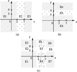
Example 3.7   Consider an application that requires two integer inputs x and y. Each of these inputs is expected to lie in the following ranges: 3 ≤ x ≤ 7 and 5 ≤ y ≤ 9. For uni-dimensional partitioning, we apply the partitioning guidelines in Tables 3.1 and 3.2 to x and y individually. This leads to the following six equivalence classes.

Figures 3.4(a) and (b) show the partitions of the input domain based on, respectively, x and y. However, we obtain the following 9 equivalence classes if we consider the input domain to be the product of X and Y, where X and Y denote, respectively, the set of values of variables x and y.

Figure 3.4 Geometric representation of equivalence classes derived using unidimensional partitioning based on x and y as in (a) and (b), respectively, and using multidimensional partitioning as in (c).

From the test selection perspective, the two unidimensional partitions generate six representative tests, one for each equivalence class. However, we obtain nine representative tests when using multidimensional partitioning. Which set of tests is better in terms of fault detection depends on the type of application.

The tests selected using multidimensional partitioning are likely to test an application more thoroughly than those selected using uni-dimensional partitioning. On the other hand, the number of equivalence classes created using multidimensional partitioning increases exponentially in the number of input variables. (See Execrises 3.8, 3.9, 3.10, and 3.11.)

3.3.5  A systematic procedure

Test selection based on equivalence partitioning can be used for small and large applications. For applications or objects involving a few variables, say 3–5, test selection could be done manually. However, as the application or object size increase to, say, 25 or more input variables, manual application becomes increasingly difficult and error prone. In such situations, the use of a tool for test selection is highly recommended.

 

The following steps are helpful in creating the equivalence classes given program requirements. The second and third steps could be followed manually or automated. The first step below, identification of the input domain, will most likely be executed manually unless the requirements have been expressed in a formal specification language such as Z in which case this step can also be automated.

1. Identify the input domain: Read the requirements carefully and identify all input and output variables, their types, and any conditions associated with their use. Environment variables, such as class variables used in the method under test and environment variables in Unix, Windows, and other operating systems, also serve as input variables. Given the set of values each variable can assume, an approximation to the input domain is the product of these sets. As we will see in Step 4, constraints specified in requirements and the design of the application to be tested will likely eliminate several elements from the input domain derived in this step.
2. Equivalence classing: Partition the set of values of each variable into disjoint subsets. Each subset is an equivalence class. Together, the equivalence classes based on an input variable partition the input domain. Partitioning the input domain using values of one variable is done based on the expected behavior of the program. Values for which the program is expected to behave in the “same way” are grouped together. Note that “same way” needs to be defined by the tester. Examples given above illustrate such grouping.
3. Combine equivalence classes: This step is usually omitted and the equivalence classes defined for each variable are directly used to select test cases. However, by not combining the equivalence classes, one misses the opportunity to generate useful tests.

   The equivalence classes are combined using the multidimensional partitioning approach described earlier. For example, suppose that program P takes two integer valued inputs denoted by X and Y. Also suppose that values of X have been partitioned into sets X₁ and X₂ while the values of Y have been partitioned into sets Y₁, Y₂, and Y₃. Taking the set product of {X₁, X₂} and {Y₁, Y₂, Y₃}, we get the following set E of six equivalence classes for P; each element of E is an equivalence class obtained by combining one equivalence class of X with another of Y.

   

   Note that this step might lead to an unmanageably large number of equivalence classes and hence is often avoided in practice. Ways to handle such an explosion in the number of equivalence classes are discussed in Sections 3.2, 4.3 (in Chapter 4), and in Chapter 6.

4. Identify infeasible equivalence classes: An infeasible equivalence class is one that contains a combination of input data that cannot be generated during a test. Such an equivalence class might arise due to several reasons. For example, suppose that an application is tested via its GUI, i.e. data is input using commands available in the GUI. The GUI might disallow invalid inputs by offering a palette of valid inputs only. There might also be constraints in the requirements that render certain equivalence classes infeasible.
   
   

   An infeasible equivalence class contains inputs that cannot be applied to the program under test.

   Infeasible data is a combination of input values that cannot be input to the application under test. Again, this might happen due to the filtering of the invalid input combinations by a GUI. While it is possible that some equivalence classes are wholly infeasible, the likely case is that each equivalence class contains a mix of testable and infeasible data.

   In this step, we remove from E equivalence classes the ones that contain infeasible inputs. The resulting set of equivalence classes is then used for the selection of tests. Care needs to be exercised while selecting tests as some data in the reduced E might also be infeasible.

Example 3.8   Let us now apply the equivalence partitioning procedure described earlier to generate equivalence classes for the software control portion of a boiler controller. A simplified set of requirements for the control portion are as follows.

Consider a boiler control system (BCS). The control software of BCS, abbreviated as CS, is required to offer one of several options. One of the options, C (for control), is used by a human operator to give one of three commands (cmd): change the boiler temperature (temp), shut down the boiler (shut), and cancel the request (cancel). Command temp causes CS to ask the operator to enter the amount by which the temperature is to be changed (tempch). Values of tempch are in the range [–10, 10] in increments of 5 degrees Fahrenheit. A temperature change of 0 is not an option.

Selection of option C forces the BCS to examine V. If V is set to GUI, the operator is asked to enter one of the three commands via a GUI. However, if V is set to file, BCS obtains the command from a command file.

The command file may contain any one of the three commands, together with the value of the temperature to be changed if the command is temp. The file name is obtained from variable F. Values of V and F can be altered by a different module in BCS. In response to temp and shut commands, the control software is required to generate appropriate signals to be sent to the boiler heating system.

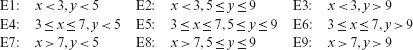
We assume that the control software is to be tested in a simulated environment. The tester takes on the role of an operator and interacts with the CS via a GUI. The GUI forces the tester to select from a limited set of values as specified in the requirements. For example, the only options available for the value of tempch are –10, –5, 5, and 10. We refer to these four values of tempch as t_valid while all other values as t_invalid. Figure 3.5 is a schematic of the GUI, the control software under test, and the input variables.

Figure 3.5 Inputs to the boiler control software. V and F are environment variables. Values of cmd (command) and tempch (temperature change) are input via the GUI or a data file depending on V. F specifies the data file.

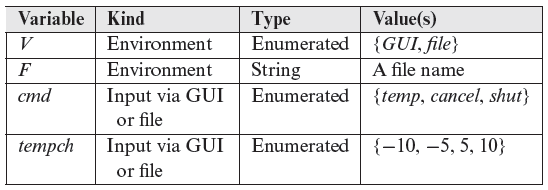
Identify the input domain: The first step in generating equivalence partitions is to identify the (approximate) input domain. Recall that the domain identified in this step will likely be a superset of the true input domain of the control software. First we examine the requirements and identify input variables, their types, and values. These are listed in the following table.

While deriving equivalence classes, it is useful to consider illegal values as possible inputs.

Considering that each variable name defines a set, we derive the following set as a product of the four variables listed above.

 

S = V × F × cmd × tempch.

 

The input domain of BCS, denoted by I, contains S. Sample values in I, and in S, are given below where the underscore character (_) denotes a “don’t care” value.

 

(GUI,_, temp,−5), (GUI,_, cancel,_), (file, cmd_ file, shut,_)

 

The following 4-tuple belongs to I but not to S.

 

(file, cmd_file, temp, 0)

 

Equivalence classing: Equivalence classes for each variable are given in the table below. Recall that for variables that are of an enumerated type, each value belongs to a distinct partition.

Variable	Partition
V	{{GUI}, {file}, {undefined}}
F	f_valid, f_invalid
cmd	{{temp}, {cancel}, {shut}, c_invalid}
tempch	{{−10}, {−5}, {5}, {10}, t_invalid}

f_valid denotes a set of names of files that exist, f_invalid denotes the set of names of nonexistent files, c_invalid denotes the set of invalid commands specified in F, t_invalid denotes the set of out of range values of tempch in the file, and undefined indicates that the environment variable V is undefined. Note that f_valid, f_ invalid, c_invalid, and t_invalid denote sets of values, whereas undefined is a singleton indicating that V is undefined.

 

Combine equivalence classes: Variables V, F, cmd, and tempch have been partitioned into 3, 2, 4, and 5 subsets, respectively. Set product of these four variables leads to a total of 3 × 2 × 4 × 5 = 120 equivalence classes. A sample follows.

 

{(GUI, f_valid, temp, −10)}, {(GUI, f_valid, temp, t_invalid)},

{(file, f_invalid, c_invalid, 5)}, {(undefined, f_valid, temp, t_invalid)},

{(file, f_valid, temp, −10)}, {(file, f_valid, temp, −5)}

 

Note that each of the classes listed above represents an infinite number of input values for the control software. For example, {(GUI, f_valid, temp, –10)} denotes an infinite set of values obtained by replacing f_valid by a string that corresponds to the name of an existing file. As we shall see later, each value in an equivalence class is a potential test input for the control software.

Discard infeasible equivalence classes: Note that the amount by which the boiler temperature is to be changed is needed only when the operator selects temp for cmd. Thus, several equivalence classes that match the following template are infeasible.

 

{(V,F, {cancel, shut, c_invalid}, t_valid ∪ t_invalid)}

 

This parent–child relationship between cmd and tempch renders infeasible a total of 3 × 2 × 3 × 5 = 90 equivalence classes.

Next, we observe that the GUI does not allow invalid values of temperature change to be input. This leads to two more infeasible equivalence classes given below.

 

{(GUI, f_valid, temp, t_invalid)} {(GUI, f_invalid, temp, t_invalid)}

The GUI does not allow invalid values of temperature change to be input.

 

Continuing with a similar argument, we observe that a carefully designed application might not ask for the values of cmd and tempch when V = file and F contains a file name that does not exist. In this case, five additional equivalence classes are rendered infeasible. Each of these five classes is described by the following template:

 

{(file, f_invalid, temp, t_valid ∪ t_invalid)}.

 

Along similar lines as above, we can argue that the application will not allow values of cmd and tempch to be input when V is undefined. Thus, yet another five equivalence classes that match the following template are rendered infeasible:

 

{(undefined, _, temp, t_valid ∪ t_invalid)}.

 

Note that even when V is undefined, F can be set to a string that may or may not represent a valid file name.

The above discussion leads us to discard a total of 90 + 2 + 5 + 5 = 102 equivalence classes. We are now left with only 18 testable equivalence classes. Of course, our assumption in discarding 102 classes is that the application is designed so that certain combinations of input values are impossible to achieve while testing the control software. In the absence of this assumption, all 120 equivalence classes are potentially testable.

The set of 18 testable equivalence classes match the seven templates listed below. The “_” symbol indicates, as before, that the data can be input but is not used by the control software, and NA indicates that the data cannot be input to the control software because the GUI does not ask for it.

 

{(GUI, f_valid, temp, t_valid)}	4 equivalence classes.
{(GUI, f_invalid, temp, t_valid)}	4 equivalence classes.
{(GUI, __, cancel, NA)}	2 equivalence classes.
{(file, f_valid, temp, t_valid ∪ t_invalid)}	5 equivalence classes.
{(file, f_valid, shut, NA)}	1 equivalence classes.
{(file, f_invalid, NA, NA)}	1 equivalence class.
{(undefined, NA, NA, NA)}	1 equivalence class.

 

There are several input data tuples that contain don’t care values. For example, if V = GUI, then the value of F is not expected to have any impact on the behavior of the control software. However, as explained in the following section, a tester must interpret such requirements carefully.

3.3.6  Test selection

Given a set of equivalence classes that form a partition of the input domain, it is relatively straightforward to select tests. However, complications could arise in the presence of infeasible data and don’t care values. In the most general case, a tester simply selects one test that serves as a representative of each equivalence class. Thus, for example, we select four tests, one from each equivalence class defined by the pCat relation in Example 3.4. Each test is a string that denotes the make and model of a printer belonging to one of the three classes or is an invalid string. Thus, the following is a set of four tests selected from the input domain of program pTest.

 

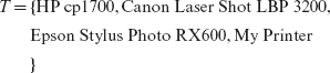
While testing pTest against tests in T, we assume that if pTest correctly selects a script for each printer in T, then it will select correct scripts for all printers in its database. Similarly, from the six equivalence classes in Example 3.5, we generate the following set Τ consisting of six tests each of the form (w,ƒ), where w denotes the value of an input word and ƒ a file name.

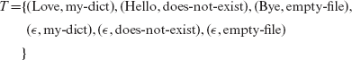
In the test above, ∊ denotes an empty, or a null, string, implying that the input word is a null string. Values of ƒ my-dict, does-not-exist, and empty-file correspond to names of files that, respectively, exist, do not exist, and exist but is empty.

Selection of tests for the boiler control software in Example 3.8 is a bit more tricky due to the presence of infeasible data and don’t care values. The next example illustrates how to proceed with test selection for the boiler control software.

 

Example 3.9   Recall that we began by partitioning the input domain of the boiler control software into 120 equivalence classes. A straightforward way to select tests would have been to pick one representative of each class. However, due to the existence of infeasible equivalence classes, this process would lead to tests that are infeasible. We therefore derive tests from the reduced set of equivalence classes. This set contains only feasible classes. Table 3.3 lists 18 tests derived from the 18 equivalence classes listed earlier in Example 3.8. The equivalence classes are labeled as E1, E2, and so on for ease of reference.

While deriving the test data in Table 3.3, we have specified arbitrary values of variables that are not expected to be used by the control software. For example, in E9, the value of F is not used. However, to generate a complete test data item, we have arbitrarily assigned to F a string that represents the name of an existing file. Similarly, the value of tempch is arbitrarily set to –5.

 

Table 3.3 Test data for the control software of a boiler control system in Example 3.8.

ID	Equivalence class* {(V, F, cmd, tempch)}	Test data† (V, F, cmd, tempch)
E1 E2 E3 E4	{(GUI, f_valid, temp, t_valid)} {(GUI, f_valid, temp, t_valid)} {(GUI, f_valid,temp, t_valid)} {(GUI, f_valid,temp, t_valid)}	(GUI, a_ file, temp, −10) (GUI, a_ file, temp, −5) (GUI, a_ file, temp, 5) (GUI, a_ file, temp, 10)
E5 E6 E7 E8	{(GUI, f_invalid temp, t_valid)} {(GUI, f_invalid temp, t_valid)} {(GUI, f_invalid temp, t_valid)} {(GUI, f_invalid temp, t_valid)}	(GUI, no_ file, temp, −10) (GUI, no_ file, temp, −10) (GUI, no_ file, temp, −10) (GUI, no_ file, temp, −10)
E9 E10	{(GUI, _, cancel, NA)} {(GUI, _, cancel, NA)}	(GUI, a_ file, cancel, −5) (GUI, no_ file, cancel, −5)
E11 E12 E13 E14 E15	{(file, f_valid, temp, t_valid)} {(file, f_valid, temp, t_valid)} {(file, f_valid, temp, t_valid)} {(file, f_valid, temp, t_valid)} {(file, f_valid, temp, t_invalid)}	(file, a_ file, temp, −10) (file, a_ file, temp, −5) (file, a_ file, temp, 5) (file, a_ file, temp, 10) (file, a_ file, temp, −25)
E16	{(file, f_valid, temp, NA)}	(file, a_ file, shut, 10)
E17	{(file, f_invalid, NA, NA)}	(file, no_ file, shut, 10)
E18	{(undefined, _, NA, NA)}	(undefined, no_ file, shut, 10)

 

The don’t care values in an equivalence class must be treated carefully. It is from the requirements that we conclude that a variable is or is not don’t care. However, an incorrect implementation might actually make use of the value of a don’t care variable. In fact, even a correct implementation might use the value of a variable marked as don’t care. This latter case could arise if the requirements are incorrect or ambiguous. In any case, it is recommended that one should assign data to don’t care variables, given the possibility that the program may be erroneous and hence make use of the assigned data value.

 

In Step 3 of the procedure, to generate equivalence classes of an input domain, we suggested the product of the equivalence classes derived for each input variable. This procedure may lead to a large number of equivalence classes. One approach to test selection that avoids the explosion in the number of equivalence classes is to cover each equivalence class of each variable by a small number of tests. We say that a test input covers an equivalence class Ε for some variable V, if it contains a representative of E. Thus, one test input may cover multiple equivalence classes one for each input variable. The next example illustrates this method for the boiler example.

 

Example 3.10   In Example 3.8, 3, 2, 4, and 5 equivalence classes were derived, respectively, for variables V, F, cmd, and tempch. The total number of equivalence classes is only 14; compare this with 120 derived using the product of individual equivalence classes. Note that we have five equivalence classes, and not just two, for variable tempch, because it is an enumerated type. The following set Τ of five tests cover each of the 14 equivalence classes.

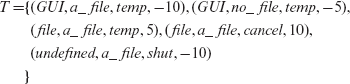
You may verify that indeed the tests listed above cover each equivalence class of each variable. While small, the above test set has several weaknesses. While the test covers all individual equivalence classes, it fails to consider the semantic relations amongst the different variables. For example, the last of the tests listed above will not be able to test the shut command assuming that the value undefined of the environment variable V is processed correctly.

Several other weaknesses can be identified in Τ of Example 3.10. The lesson to be learned from this example is that one must be careful, i.e. consider the relationships amongst variables, while deriving tests that cover equivalence classes for each variable. In fact, it is easy to show that a small subset of tests from Table 3.3 will cover all equivalence classes of each variable and satisfy the desired relationships amongst the variables. (See Exercise 3.13.)

3.3.7  Impact of GUI design

Test selection is usually affected by the overall design of the application under test. Prior to the development of graphical user interfaces (GUI), data was input to most programs in textual forms through typing on a keyboard, or many many years ago, via punched cards. Most applications of today, either new or refurbished, exploit the advancements in GUI to make interaction with programs much easier and safer than before. Test design must account for the constraints imposed on data by the front-end application GUI.

 

While designing equivalence classes for programs that obtain input exclusively from a keyboard, one must account for the possibility of errors in data entry. For example, suppose that the requirement for an application A places a constraint on an input variable X such that it can assume integral values in the range [0, 0.4]. However, a user of this application may inadvertently enter a value for X that is out of range. While the application is supposed to check for incorrect inputs, it might fail to do so. Hence, in test selection using equivalence partitioning, one needs to test the application using at least three values of X, one that falls in the required range and two that fall outside the range on either side. Thus, three equivalence classes for X are needed. Figure 3.6(a) illustrates this situation where the “Incorrect values” portion of the input domain contains the out of range values for X.

However, suppose that all data entry to application A is via a GUI front end. Suppose also that the GUI offers exactly five correct choices to the user for X. In such a situation, it is impossible to test A with a value of X that is out of range. Hence only the correct values of X will be input to A. This situation is illustrated in Figure 3.6(b).

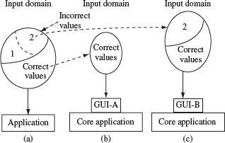
Figure 3.6 Restriction of the input domain through careful design of the GUI. Partitioning of the input domain into equivalence classes must account for the presence of GUI as shown in (b) and (c). GUI-Α protects all variables against incorrect input while GUI-B does allow the possibility of incorrect input for some variables.

Of course, one could dissect the GUI from the core application and test the core separately with correct and incorrect values of X. But any error so discovered in processing incorrect values of X might be meaningless because, as a developer may argue, in practice the GUI would prevent the core of A from receiving an invalid input for X. In such a situation, there is no need to define an equivalence class that contains incorrect values of an input variable.

 

In some cases, a GUI might ask the user to type in the value of a variable in a text box. In a situation like this one must certainly test the application with one or more incorrect values of the input variable. For example, while testing, it is recommended that one use at least three values for X. In case the behavior of A is expected to be different for each integer within the range [0, 4], then A should be tested separately for each value in the range as well as at least two values outside the range. However, one need not include incorrect values of variables in a test case if the variable is protected by the GUI against incorrect input. This situation is illustrated in Figure 3.6(c) where the subset labeled 1 in the set of incorrect values need not be included in the test data while values from subset labeled 2 must be included.

The above discussion leads to the conclusion that test design must take into account GUI design. In some cases, GUI design requirements could be dictated by test design. For example, GUI design might require that whenever possible only valid values be offered as options to the user. Certainly, the GUI needs to be tested separately against such requirements. The boiler control example given earlier shows that the number of tests can be reduced significantly if the GUI prevents invalid inputs from getting into the application under test.

Note that the tests derived in the boiler example make the assumption that the GUI has been correctly implemented and does prohibit incorrect values from entering the control software.

3.4  Boundary Value Analysis

Experience indicates that programmers make mistakes in processing values at or near the boundaries of equivalence classes. For example, suppose that method Μ is required to compute a function f₁ when the condition x ≤ 0 is satisfied by input x and function f₂ otherwise. However, Μ has an error due to which it computes f₁ for x ≤ 0 and f₂ otherwise. Obviously, this fault is revealed, though not necessarily, when Μ is tested against x = 0 but not if the input test set is, for example, {–4, 7} derived using equivalence partitioning. In this example, the value x = 0, lies at the boundary of the equivalence classes x ≤ 0 and x > 0.

 

Boundary value analysis is a test selection technique that targets faults in applications at the boundaries of equivalence classes. While equivalence partitioning selects tests from within equivalence classes, boundary value analysis focuses on tests at and near the boundaries of equivalence classes. Certainly, tests derived using either of the two techniques may overlap.

Test selection using boundary value analysis is generally done in conjunction with equivalence partitioning. However, in addition to identifying boundaries using equivalence classes, it is also possible and recommended that boundaries be identified based on the relations amongst the input variables. Once the input domain has been identified, test selection using boundary value analysis proceeds as follows.

1. Partition the input domain using unidimensional partitioning. This leads to as many partitions as there are input variables. Alternately, a single partition of an input domain can be created using multidimensional partitioning.
2. Identify the boundaries for each partition. Boundaries may also be identified using special relationships amongst the inputs.
3. Select test data such that each boundary value occurs in at least one test input. An illustrative example to generate tests using boundary value analysis follows.
   
   

   While tests derived using boundary value analysis will likely be in one or more equivalence partitions, they might not have been selected using the equivalence partitioning method.

Example 3.11   This simple example is to illustrate the notion of boundaries and selection of tests at and near the boundaries. Consider a method fP, brief for find Price, that takes two inputs code and qty. The item code is represented by the integer code and the quantity purchased by another integer variable qty. fP accesses a database to find and display the unit price, description, and the total price of the item corresponding to code. fP is required to display an error message, and return, if either of the two inputs is incorrect. We are required to generate test data to test fP.

We start by creating equivalence classes for the two input variables. Assuming that an item code must be in the range [99, 999] and quantity in the range [1, 100], we obtain the following equivalence classes.

 

Equivalence classes for code:	E1: Values less than 99. E2: Values in the range. E3: Values greater than 999.
Equivalence classes for qty:	E4: Values less than 1. E5: Values in the range. E6: Values greater than 100.

 

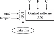
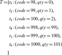
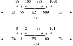
Figure 3.7 shows the equivalence classes for code and qty and the respective boundaries. Notice that there are two boundaries each for code and qty. Marked in the figure are six points for each variable, two at the boundary marked “x”, and four near the boundaries marked “*”. Test selection based on the boundary value analysis technique requires that tests must include, for each variable, values at and around the boundary. Usually, several sets of tests will satisfy this requirement. Consider the following set.

In some cases each equivalence class might contain exactly one element which is also at the boundary of the variable under consideration. The equivalence class containing a sole empty string is one example of such a class.

Figure 3.7 Equivalence classes and boundaries for variables (a) code and (b) qty in Example 3.11. Values at and near the boundary are listed and marked with an “x” and “*” respectively.

 

Each of the six values for each variable is included in the tests above. Notice that the illegal values of code and qty are included in the same test. For example, tests t₁ and t₆ contain illegal values for both code and qty and require that fP display an error message when executed against these tests. Tests t₂, t₃, t₄ and t₅ contain legal values. 

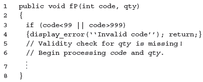
While T is a minimal set of tests that include all boundary and near-boundary points for code and qty, it is not the best when evaluated against its ability to detect faults. Consider, for example, the following faulty code skeleton for method fP.

When fP that includes the above code segment is executed against t₁ or t₆, it will correctly display an error message. This behavior would indicate that the value of code is incorrect. However, these two tests fail to check that the validity check on qty is missing from the program. None of the other tests will be able to reveal the missing code error. By separating the correct and incorrect values of different input variables, we increase the possibility of detecting the missing code error.

It is also possible that the check for the validity of code is missing but that for checking the validity of qty exists and is correct. Keeping the two possibilities in view, we generate the following four tests that can safely replace t₁ and t₆ listed above. The following two tests are also derived using boundary value analysis.

 

t₇ = (code = 98, qty = 45)

t₈ = (code = 1000, qty = 45)

t₉ = (code = 250, qty = 0)

t₁₀ = (code = 250, qty = 101)

 

One could improve the chances of detecting a missing code by separating the tests for legal and illegal values of different input variables.

A test suite for fP, derived using boundary value analysis, now consists of t₂, t₃, t₄, t₅, t₇, t₈, t₉, and t₁₀. If there is a reason to believe that tests that include boundary values of both inputs might miss some error, then tests t₂ and t₆ must also be replaced to avoid the boundary values of code and qty from appearing in the same test. (See Exercise 3.17.)

 

Example 3.12   Consider a method named textSearch to search for a non-empty string s in text txt. Position of characters in txt begins with 0 representing the first character, 1 the next character, and so on. Both s and txt are supplied as parameters to textSearch. The method returns an integer p such that if p ≥ 0, then it denotes the starting position of s in txt. A negative value of p implies that s is not found in txt.

To apply the boundary value analysis technique, we first construct the equivalence classes for each input variable. In this case, both inputs are strings and no constraints have been specified on their length or contents. Based on the guidelines in Tables 3.1 and 3.2, we arrive at the following four equivalence classes for s and txt.

 

Equivalence classes for s: E₁: empty string, E₂: non-empty string.

Equivalence classes for txt: E₃: empty string, E₄: non-empty string.

It is possible to define boundaries for a string variable based on its length and semantics. In this example, the lower bound on the lengths of both s and txt is 0 and hence this defines one boundary for each input. No upper bound is specified on lengths of either variable. Hence, we obtain only one boundary case for each of the two inputs. However, as is easy to observe, E₁ and E₃ contain exactly the boundary case. Thus, tests derived using equivalence partitioning on input variables are the same as those derived by applying boundary value analysis.

Let us now partition the output space of textSearch into equivalence classes. We obtain the following two equivalence classes for p:

 

E₅: p < 0, E₆: p ≥ 0.

 

To obtain an output that belongs to E₅, the input string s must not be in txt. Also, to obtain an output value that falls into E₆, input s must be in txt. As both E₅ and E₆ are open ranges, we obtain only one boundary, p = 0 based on E₅ and E₆. A test input that causes a correct textSearch to output p = 0 must satisfy two conditions: (i) s must be in txt and (ii) s must appear at the start of txt. These two conditions allow us to generate the following test input based on boundary value analysis:

 

s = “Laughter” and txt =“Laughter is good for the heart.”

 

Based on the six equivalence classes and two boundaries derived, we obtain the following set Τ of three test inputs for textSearch.

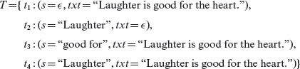
It is easy to verify that tests t₁ and t₂ cover equivalence classes E₁, E₂, E₃, E₄, and E₅ and t₃ covers E₆. Test t₄ is necessitated by the conditions imposed by boundary value analysis. Notice that none of the six equivalence classes requires us to generate t₄. However, boundary value analysis, based on output equivalence classes E₅ and E₆, requires us to generate a test in which s occurs at the start of txt.

Test t₄ suggests that we add to T yet another test t₅ where s occurs at the end of txt.

 

t₅ : (s = “heart.”, txt = “Laughter is good for the heart.”)

 

None of the six equivalence classes derived above, or the boundaries of those equivalence classes, directly suggest t₅. However, both t₄ and t₅ aim at ensuring that textSearch behaves correctly when s occurs at the boundaries of txt.

Having tests on the two boundaries determined using s and txt, we now examine test inputs that are near the boundaries. Four such cases are listed below.

• s starts at position 1 in txt. Expected output: p = 1.
• s ends at one character before the last character in txt. Expected output: p = k, where k is the position from where s starts in txt.
• All but the first character of s occur in txt starting at position 0. Expected output: p = –1.
• All but the last character of s occur in txt at the end. Expected output: p = –1.

The following tests, added to T, satisfy the four conditions listed above.

 

t₆ : (s = “aughter”, txt = “Laughter is good for the heart.”),

t₇ : (s = “heart”, txt = “Laughter is good for the heart.”),

t₈ : (s = “gLaughter”, txt = “Laughter is good for the heart.”),

t₉ : (s = “heart.d”, txt = “Laughter is good for the heart.”).

 

We now have a total of nine tests of which six are derived using boundary value analysis. Points on and off the boundary are shown in Figure 3.8. Two boundaries are labeled 1 and 2 and four points off the boundaries are labeled 3, 4, 5, and 6.

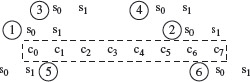
Figure 3.8 c₀ through c₇ are the eight characters in txt starting at the leftmost position 0. s₀s₁ is the input string s. Shown here is the positioning of s with respect to txt at the two boundaries, labeled 1 and 2, and at four points near the boundary, labeled 3 through 6.

Next, one might try to obtain additional tests by combining the equivalence classes for s and txt. This operation leads to four equivalence classes for the input domain of textSearch as listed below.

 

E₁ × E₃, E₁ × E₄, E₂ × E₃, E₂ × E₄.

 

Tests t₁, t₂ and t₃ cover all the four equivalence classes except for E₁ × E₃. We need the following test to cover E₁ × E₃.

 

t₆ : (s = ∊, txt = ∊).

 

Thus, combining the equivalence classes of individual variables has led to the selection of an additional test case. Of course, one could have derived t₆ based on E₁ and E₃ also. However, coverage of E₁ × E₃ requires t₆, whereas coverage of E₁ and E₃ separately does not. Notice also that test t₄ has a special property that is not required to hold if we were to generate a test that covers the four equivalence classes obtained by combining the equivalence classes for individual variables.

The previous example leads to the following observations:

• Relationships amongst the input variables must be examined carefully while identifying boundaries along the input domain. This examination may lead to boundaries that are not evident from equivalence classes obtained from the input and output variables.
• Additional tests may be obtained when using a partition of the input domain obtained by taking the product of equivalence classes created using individual variables.

3.5  Category-Partition Method

The category-partition method is a systematic approach to the generation of tests from requirements. The method consists of a mix of manual and automated steps. Here, we describe the various steps in using the category-partition method and illustrate with a simple running example.

 

3.5.1  Steps in the category-partition method

The category-partition method consists of eight steps as shown in Figure 3.9. In essence, a tester transforms requirements into test specifications. These test specifications consist of categories corresponding to program inputs and environment objects.

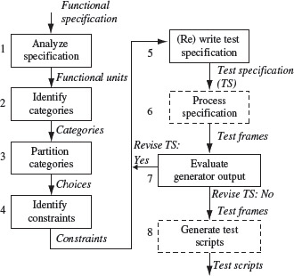
Figure 3.9 Steps in the generation of tests using the category-partition method. Tasks in solid boxes are performed manually and generally difficult to automate. Dashed boxes indicate tasks that can be automated.

Each category is partitioned into choices that correspond to one or more values for the input or the state of an environment object. Test specifications also contain constraints on the choices so that only reasonable and valid sets of tests are generated. Test specifications are input to a test frame generator that produces a number of test frames from which test scripts are generated. A test frame is a collection of choices, one corresponding to each category. A test frame serves as a template for one or more test cases that are combined into one or more test scripts.

 

A running example is used here to describe the steps shown in Figure 3.9. We use the findPrice function used in Example 3.11. The requirements for the findPrice function are expanded below for the purpose of illustrating the category-partition method.

 

Function: findPrice

 

Syntax: fP(code, quantity, weight)

 

Description:

 

findPrice takes three inputs: code, qty, and weight. Item code is represented by a string of eight digits contained in variable code. The quantity purchased is contained in qty. The weight of the item purchased is contained in weight.

Function fP accesses a database to find and display the unit price, the description, and the total price of the item corresponding to code. fP is required to display an error message, and return, if either of the three inputs is incorrect. As indicated below, the leftmost digit of code decides how the values of qty and weight are to be used, code is an 8-digit string that denotes product type. fP is concerned with only the leftmost digit that is interpreted as follows.

Leftmost digit	Interpretation
0	Ordinary grocery items such as bread, magazines, and soap.
2	Variable-weight items such as meats, fruits, and vegetables.
3	Health-related items such as Tylenol, Bandaids, and Tampons.
5	Coupon; digit 2 (dollars), 3 and 4 (cents) specify the discount.
1, 6–9	Unused

The use of parameters qty and weight depends on the leftmost digit in code. qty indicates the quantity purchased, an integer, when the leftmost digit is 0 or 3; weight is ignored. weight is the weight of the item purchased when the leftmost digit is 2; qty is ignored. qty is the value of the discount when the leftmost digit is 5; again weight is ignored. We assume that digits 1, and 6 through 9, are ignored. When the leftmost digit is 5, the second digit from the left specifies the dollar amount and the third and fourth digits the cents.

Step 1: Analyze specification

In this step, the tester identifies each functional unit that can be tested separately. For large systems, a functional unit may correspond to a subsystem that can be tested independently. The subsystem can be further subdivided leading eventually to independently testable subunits. The subdivision process terminates depending on what is to be tested.

 

Example 3.13   In this example, we assume that fP is an independently testable subunit of an application. Thus, we will derive tests for ƒP.

Step 2: Identify categories

For each testable unit, the given specification is analyzed and the inputs isolated. In addition, objects in the environment, e.g. a file, also need to be identified.

Next, we determine characteristics of each parameter and environmental object. A characteristic is also referred to as a category. While some characteristics are stated explicitly, others might need to be derived by a careful examination of the specification.

 

Example 3.14   We note that fP has three input parameters: code, qty, and weight. The specification mentions various characteristics of these parameters such as their type and interpretation. Notice that qty and weight are related to code. The specification does mention the types of different parameters but does not indicate bounds on qty and weight.

The database accessed by fP is an environment object. No characteristics of this object are mentioned in the specification. However, for a thorough testing of fP, we need to make assumptions about the existence or non-existence of items in the database. We identify the following categories for fP.

code: length, leftmost digit, remaining digits

qty: integer-quantity

weight: float-quantity

database: contents

Notice that we have only one category each for qty, weight, and database. In the next step, we see how to partition these categories.

Step 3: Partition categories

For each category the tester determines different cases against which the functional unit must be tested. Each case is also referred to as a choice. One or more cases are expected for each category. It is useful to partition each category into at least two subsets, a set containing correct values and another consisting of erroneous values.

 

In the case of a networked application, cases such as network failure ought to be considered. Other possible cases of failure, e.g. database unavailable, also need to be considered. It is for the tester to think of reasonable situations, both valid and invalid, that might arise when the unit under test is in actual use.

 

Example 3.15   Following is a summary of the various inputs, environment objects, categories, and partitions.

 

Parameters:

Environments:

database:

contents

      item exists

      item does not exist

Notice that if fP were to operate in a networked environment, then several other cases are possible. We leave these to Exercise 3.20.

Step 4: Identify constraints

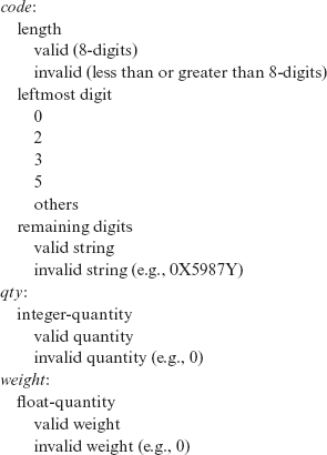
A test for a functional unit consists of a combination of choices for each parameter and environment object. Certain combinations might not be possible while others must satisfy specific relationships. In any case, constraints amongst choices are specified in this step. These constraints are used by the test generator to produce only the valid test frames in Step 6.

 

A constraint is specified using a property list and a selector expression. A property list has the following form:

 

[property P1, P2,..]

 

where “property” is a key word and P1, P2, etc. are names of individual properties. Each choice can be assigned a property. A selector expression is a conjunction of pre-defined properties specified in some property list. A selector expression takes one of the following forms:

 

[if P1]

[if P1 and P2 and . . .]

 

The above two forms can be suffixed to any choice. A special property written as [error] can be assigned to choices that represent error conditions. Another special property written as [single] allows the tester to specify that the associated choice is not to be combined with choices of other parameters, or environment objects, while generating test frames in Step 6. 

Example 3.16   Properties and selector expressions assigned to a few choices sampled from Example 3.15 follow; comment lines start with #.

# Leftmost digit of code
0	[property ordinary-grocery]
2	[property variable-weight]
# Remaining digits of code
valid string	[single]
# Valid value of qty
valid quantity	[if ordinary-grocery]
# Invalid value of qty
invalid quantity	[error]

Step 5: (Re) write test specification

Having assigned properties and selector expressions to various choices, the tester now writes a complete test specification. The specification is written in a test specification language (TSL) conforming to a precise syntax.

This step may need to be executed more than once in the event the tester is not satisfied with the test frames generated in Step 6. This happens when the tester evaluates the test frames in Step 7 and finds that some test frames are redundant. Such frames may have been generated by combining choices that are either impractical or unlikely to arise in practice. In such an event, the tester rewrites the specification and inputs them for processing in Step 6.

 

Example 3.17   A complete test specification for fP follows; we have ignored the processing coupon category (see Exercise 3.21). We have used a slight variation of the TSL syntax as given by Ostrand and Balcer (also see Bibliographic notes).

 

Parameters:

Environments:

database

  item exists

  item does not exist [error]

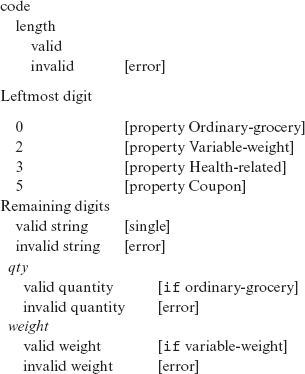
Step 6: Process specification

The TSL specification written in Step 5 is processed by an automatic test frame generator. This results in a number of test frames. The test frames are analyzed by the tester for redundancy, i.e. they might test the application in the same way. In such cases, one either rewrites the test specifications or simply ignores the redundant frames. 

Example 3.18   A sample test frame generated from the test specification in Example 3.17 follows.

 

Test case 2: (Key = 1.2.1.0.1.1)

Length:	valid
Leftmost digit:	2
Remaining digits:	valid string
qty:	ignored
weight:	3.19
database:	item exists

 

A test number identifies the test. The key in a test frame indicates the choices used, a 0 indicating no choice. qty is ignored as the leftmost digit corresponds to a variable weight item that is priced by weight and not by quantity. (Note that the terminology used in this example differs from that in the original TSL.)

A test frame is not a test case. However, a test case, consisting of specific input values and expected outputs, can be derived from a test frame. It is important to note that the test frame contains information about the environment objects. Hence, it is useful in setting up the environment prior to a test.

 

Test frames are generated by generating all possible combinations of choices while satisfying the constraints. Choices that are marked error or single are not combined with others and produce only one test case. It is easy to observe that without any constraints (selector expressions), a total of 128 test frames will be generated from the specification in Example 3.17.

Step 7: Evaluate generator output

In this step, the tester examines the test frames for any redundancy or missing cases. This might lead to a modification in the test specification (Step 5) and a return to Step 6.

Step 8: Generate test scripts

Test cases generated from test frames are combined into test scripts. A test script is a grouping of test cases. Generally, test cases that do not require any changes in settings of the environment objects are grouped together. This enables a test driver to efficiently execute the tests.

That completes our description of the category-partition method. As you may have noticed, the method is essentially a systematization of the equivalence partitioning and boundary value techniques discussed earlier.

Writing a test specification allows a test team to take a close look at the program specifications. For large systems, this task can be divided amongst members of the test team. While a significant part of the method requires manual work, availability of a tool that processes TSL specifications helps in test generation and documentation. It also reduces the chances of errors in test cases.

 

Exercises

3.1 Let N be the size of a sequence s of integers. Assume that an element of s can be any one of v distinct values. Show that the number of possible sequences is

3.2 An equivalence relation R on set S is reflexive, symmetric, and transitive. Also, R partitions S into equivalence classes. Show that each of the relations defined in Exercises 3.3 and 3.4 is an equivalence relation.

3.3 Derive equivalence classes for the input variables listed below.

• int pen_inventory; Current inventory level of writing pens.
• string planet_name; Planet name.
• operating_system={“OS X”, “Windows XP”, “Windows 2000”,
  “Unix”, “Linux”, “Xinu”, “VxWorks”}; Name of an operating system.
• printer_class=set printer_name;
  printer_class p; Set of printer names.
• int name [1.10]; An array of at most 10 integers.

3.4 In Example 3.4, suppose now that we add another category of printers, say, “Home and home office (hb).” Define a suitable relation hb that partitions the input domain of pTest into two equivalence classes. Discuss the overlap of the equivalence classes induced by hb with the remaining eight classes defined by the four relations in Example 3.4.

3.5 Consider the following relation
cl : I → {yes, no}

cl maps an input domain I of pTest in Example 3.4 to the set {yes, no}. A printer make and model is mapped to yes if it is a color laserjet, else it is mapped to no. Is cl an equivalence relation?

3.6 (a) Why consider classes E2–E6 in Example 3.5 when the correctness of the program corresponding to tests in these classes can be verified by simple inspection? Offer at least two reasons.
(b) Are there any additional equivalence classes that one ought to consider while partitioning the input domain of wordCount?

3.7 Partition the input domain of the transcript component described in Example 3.6 into equivalence classes using the guidelines in Tables 3.1 and 3.2. Note that transcript takes two inputs, a record R and an integer N.

3.8 (a) Generate two sets of tests T₁ and T₂ from the partitions created in Example 3.7 using, respectively, uni-dimensional and multidimensional partitioning. Which of the following relations holds amongst T₁ and T₂ that you have created: and T₁ = T₂, T₁ ⊂ T₂, T₁ ⊆ T₂, T₁ ⊃ T_2, T₁ ⊇ T₂, and T₁ ≠ T₂? (b) Which of the six relations mentioned could hold between T₁ and T₂ assuming that T₁ is derived from equivalence classes constructed using uni-dimensional partitioning and T₂ using multidimensional partitioning?

3.9 Consider an application App that takes two inputs name and age where name is a non-empty string containing at most 20 alphabetic characters and age is an integer that must satisfy the constraint 0 ≤ age ≤ 120. App is required to display an error message if the input value provided for age is out of range. It truncates any name that is more than 20 characters in length and generates an error message if an empty string is supplied for name.

Partition the input domain using (a) uni-dimensional partitioning and (b) multidimensional partitioning. Construct two sets of test data for App using the equivalence classes derived in (a) and in (b).

3.10 Suppose that an application has m input variables and that each variable partitions the input space into n equivalence classes. The multidimensional partitioning approach will divide the input domain into how many equivalence classes?

3.11 An application takes two inputs x and y where x ≤ y and –5 ≤ y ≤ 4. (a) Partition the input domain using uni-dimensional and multidimensional partitioning. (b) Derive test sets based on the partitions created in (a).

3.12 In Example 3.8, we started out by calculating the number of equivalence classes to be 120. We did so because we did not account for the parent-child relationship between cmd and tempch. Given this relationship, how many equivalence classes should we start out with in the first step of the procedure for partitioning the input domain into equivalence classes?

3.13

• Identify weaknesses, as many as you can, of the test T derived in Example 3.10.
• Derive a test set that covers each individual equivalence class derived for the four variables in Example 3.8 while ensuring that the semantic relations between different variables are maintained.
• Compare the test set derived in (b) with that in Table 3.3 in terms of their respective sizes and error detection effectiveness. If you believe that the error detection effectiveness of the test set you derived is less than that of the test set in Table 3.3, then offer an example of an error in the boiler control software that will likely be not detected by your test set but will likely be detected by the test set in Table 3.3.

3.14 An object named compute takes an integer x as input. It is required to send a message to another object 0₁ if x ≤ 0 and a message to object O₂ if x > 0. However, due to an error in compute, a message is sent to to O₁ when x < 0 and to O₂ otherwise. Under what condition(s) will the input x = 0 not reveal the error in compute?

3.15 For each test t ∊ Τ in Example 3.12, construct one example of a fault in textSearch that is guaranteed to be detected only by t. Hint: Avoid trivial examples !

3.16 A method named cC takes three inputs: from, to, and amount. Both from and to are strings and denote the name of a country. Variable amount is of type float. Method cC converts amount in the currency of the country specified by from and returns the equivalent amount, a quantity of type float, in the currency of the country specified by to. Here is an example prepared on July 26, 2004:

Inputs: from = “USA”, to = “Japan”, amount = 100
Returned value: 11,012.0

(a) Derive a set of tests for cC using equivalence partitioning and boundary values analysis.

(b) Suppose that a GUI encapsulates cC and allows the user to select the values of from and to using a palette of country names. The user types in the amount to be converted in a text box before clicking on the button labeled Convert. Will the presence of the GUI change the tests you derived in (a)? If so, how? If not, why?

You may find that the requirement specification given for cC is incomplete in several respects. While generating tests, it is recommended that you resolve any ambiguities in the requirements and complete the information not available by using common sense and/or discussing the problem with appropriate members of the design/development team.

3.17 Recall the boundary value analysis in Example 3.11. (a) Construct one example of a boundary error in fP that may go undetected unless tests t₂ and t₅ are replaced so that computation at the boundaries of code and qty is checked in separate tests. (b) Replace t₂ and t₅ by an appropriate set of tests that test fP at the boundaries of code and qty in separate tests.

3.18 Compare test generation using boundary value analysis and equivalence partitioning methods described in this chapter in terms of the number of tests generated, the error detection ability, and the source of tests.

3.19 Consider the following problem for computing the monthly utility bill as formulated by Rob Hierons to illustrate coincidental correctness.

Let W and E denote, respectively, the monthly water and electricity consumption in standard units. Let C_w and C_e denote, respectively, the costs of consuming one standard unit of water and electricity. The monthly charge to the customer is computed as: (C_w * W + C_e * E). However, in situations where a customer uses at least M_w units of water, a 20% discount is applied to the electricity portion of the charge. In this case, the charge to the customer is computed as (C_w * W + 0.2 * C_e * E).

Now suppose that M_w = 30 but while coding the computation of the monthly utility charge, the programmer has used by mistake M_w = 40. Thus, instead of using the condition W ≥ 30 the programmer uses the condition W ≥ 40 to select one of the two formulae above to compute the monthly utility charges. Assume that the function under test (in Java) is as given below.

 

1   public double incorrectHierons(double w, double e, double cw, double ce){

2     final double mw=40; // Should be 30.

3     final double discount=0.2;

4     if(w>=mw){

5      return(w*cw+discount*ce*e);

6     }else{

7     return(w*cw+ce*e);

8     }

9   }

 

(a) Use boundary value analysis to determine test inputs to test the (incorrect) function to compute the utility bill. (b) Use partition testing techniques to derive the test cases to test the (incorrect) function to compute the utility bill. (c) Under what conditions will your test fail to discover the error?

3.20 In Example 3.15, suppose that fP is to be used in a checkout counter. The cash register at the counter is connected to a central database from where fP obtains the various attributes of an item such as name and price. Does this use of fP in a networked environment add to the list of environment objects? Can you think of any additional categories and different partitions?

3.21 The coupon field was ignored in the test specification derived in Example 3.17. Given the specifications on page 145, modify the test specifications in Example 3.17 so that correct tests are generated for the processing of the coupon field.