
6
Test Generation from Combinatorial Designs
CONTENTS
6.2 A combinatorial test design process
6.5 Mutually orthogonal latin squares
6.6 Pairwise design: binary factors
6.7 Pairwise design: multi-valued factors
6.9 Covering and mixed-level covering arrays
The purpose of this chapter is to introduce techniques for the generation of test configurations and test data using the combinatorial design techniques with program inputs and their values as factors and levels respectively. These techniques are useful when testing a variety of applications. They allow selection of a small set of test configurations from an often impractically large set, and are effective in detecting faults arising out of factor interactions.
6.1 Combinatorial Designs
Software applications are often designed to work in a variety of environments. Combinations of factors such as the operating system, network connection, and hardware platform, lead to a variety of environments. Each environment corresponds to a given set of values for each factor, known as a test configuration. For example, Windows XP, Dial-up connection, and a PC with 1 GB of main memory, is one possible configuration. To ensure high reliability across the intended environments, the application must be tested under as many test configurations, or environments, as possible. However, as illustrated in examples later in this chapter, the number of such test configurations could be exorbitantly large making it impossible to test the application exhaustively.
An analogous situation arises in the testing of programs that have one or more input variables. Each test run of a program often requires at least one value for each variable. For example, a program to find the greatest common divisor of two integers x and y requires two values, one corresponding to x and the other to y. In earlier chapters, we have seen how program inputs can be selected using techniques such as equivalence partitioning and boundary value analysis. While these techniques offer a set of guidelines to design test cases, they suffer from two shortcomings: (a) they raise the possibility of a large number of subdomains in the partition of the input space and (b) they lack guidelines on how to select inputs from various subdomains in the partition.
The number of subdomains in a partition of the input domain increases in direct proportion to the number and type of input variables, and especially so when multidimensional partitioning is used. Also, once a partition is determined, one selects at random a value from each of the subdomains. Such a selection procedure, especially when using unidimensional equivalence partitioning, does not account for the possibility of faults in the program under test that arise due to specific interactions amongst values of different input variables. While boundary value analysis leads to the selection of test cases that test a program at the boundaries of the input domain, other interactions in the input domain might remain untested.
This chapter describes several techniques for generating test configurations or test sets that are small even when the set of possible configurations, or the input domain, and the number of subdomains in its partition, is large and complex. The number of test configurations, or the test set so generated, has been found to be effective in the discovery of faults due to the interaction of various input variables. The techniques we describe here are known by several names such as design of experiments, combinatorial designs, orthogonal designs, interaction testing, and pairwise testing.
6.1.1 Test configuration and test set
In this chapter, we use the terms test configuration and test set interchangeably. Even though we use the terms interchangeably, they do have different meaning in the context of software testing. However, as the techniques described in this chapter apply to the generation of both test configurations as well as test sets, we have taken the liberty of using them interchangeably. One must be aware that a test configuration is usually a static selection of factors, such as the hardware platform or an operating system. Such selection is completed prior to the start of the test. In contrast, a test set is a collection of test cases used as input during the test process.
6.1.2 Modeling the input and configuration spaces
The input space of a program Ρ consists of k-tuples of values that could be input to Ρ during execution. The configuration space of Ρ consists of all possible settings of the environment variables under which Ρ could be used.
Example 6.1 Consider program Ρ that takes two integers x > 0 and y > 0 as inputs. The input space of Ρ is the set of all pairs of positive non-zero integers. Now suppose that this program is intended to be executed under the Windows and the Mac OS operating system, through the Firefox or Safari browsers, and must be able to print to a local or a networked printer. The configuration space of Ρ consists of triples (Χ, Υ, Z), where X represents an operating system, Y a browser, and Ζ a local or a networked printer.
Next, consider a program Ρ that takes n inputs corresponding to variables X1,X2, ... ,Xn. We refer to the inputs as factors. The inputs are also referred to as test parameters or as values. Let us assume that each factor may be set at any one from a total of ci, 1 ≤ i ≤ n values. Each value assignable to a factor is known as a level. The notation |F| refers to the number of levels for factor F.
The environment under which an application is intended to be used, generally contributes one or more factors. In Example 6.1, the operating system, browser, and printer connection are three factors that will likely affect the operation and performance of P.
A set of values, one for each factor, is known as a factor combination. For example, suppose that program Ρ has two input variables X and Y. Let us say that during an execution of Ρ, X and Y may each assume a value from the set {a, b, c} and {d, e, f}, respectively. Thus we have two factors and three levels for each factor. This leads to a total of 32 = 9 factor combinations, namely (a, d), (a, e), (a, f), (b, d), (b, e), (b, f), (c, d), (c, e), and (c, f). In general, for k factors with each factor assuming a value from a set of n values, the total factor combinations is nk.
Suppose now that each factor combination yields one test case. For many programs, the number of tests generated for exhaustive testing could be exorbitantly large. For example, if a program has 15 factors with four levels each, the total number of tests is 415 ≈ 109. Executing a billion tests might be impractical for many software applications.
There are special combinatorial design techniques that enable the selection of a small subset of factor combinations from the complete set. This sample is targeted at specific types of faults known as interaction faults. Before we describe how the combinatorial designs are generated, let us look at a few examples that illustrate where they are useful.
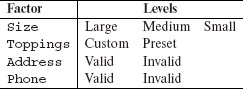
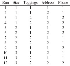
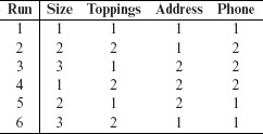
Example 6.2 Let us model the input space of an online Pizza Delivery Service (PDS) for the purpose of testing. The service takes orders online, checks for their validity, and schedules Pizza for delivery. A customer is required to specify the following four items as part of the online order: Pizza size, Toppings list, Delivery address, and a home phone number. Let us denote these four factors by S, T, A, and P, respectively.
Suppose now that there are three varieties for size: Large, Medium, and Small. There is a list of six toppings from which to select. In addition, the customer can customize the toppings. The delivery address consists of customer name, one line of address, city, and the zip code. The phone number is a numeric string possibly containing the dash (“–”) separator.
The table below lists one model of the input space for the PDS. Note that while for Size we have selected all three possible levels, we have constrained the other factors to a smaller set of levels. Thus, we are concerned with only one of two types of values for Toppings, Custom or Preset, and one of the two types of values for factors Address and Phone, namely Valid and Invalid.
The total number of factor combinations is 24 + 23 = 24 (alternately, 3 × 2 × 2 × 2 = 24). However, as an alternate to the table above, we could consider 6 + 1 = 7 levels for Toppings. This would increase the number of combinations to 24 + 5 × 23 + 23 + 5 × 22 = 84 (alternately, 3 × 7 × 2 × 2 = 84). We could also consider additional types of values for Address and Phone which would further increase the number of distinct combinations. Notice that if we were to consider each possible valid and invalid string of characters, limited only by length, as a level for Address, we will arrive at a huge number of factor combinations.
Later in this section we explain the advantages and disadvantages of limiting the number of factor combinations by partitioning the set of values for each factor into a few subsets. Notice also the similarity of this approach with equivalence partitioning. The next example illustrates factors in a Graphical User Interface (GUI).
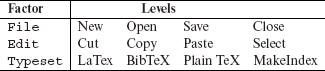
Example 6.3 The GUI of application Τ consists of three menus labeled File, Edit, and Typeset. Each menu contains several items listed below.
We have three factors in Τ. Each of these three factors can be set to any of four levels. Thus, we have a total of 43 = 64 factor combinations.
Note that each factor in this example corresponds to a relatively smaller set of levels when compared to factors Address and Phone in the previous example. Hence the number of levels for each factor is set equal to the cardinality of the set of the corresponding values.
Example 6.4 Let us now consider the Unix sort utility for sorting ASCII data in files or obtained from the standard input. The utility has several options and makes an interesting example for the identification of factors and levels. The command line for sort is as given below.
sort [ -cmu ] [ -o output ] [ -T directory ] [ -y [ kmem ]] [ -z recsz ] [ -dfiMnr ] [ - b ] [ t char ] [ -k keydef ] [ +pos1 [ -pos2 ]] [ file…]
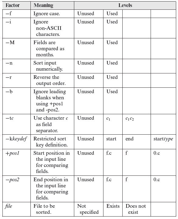
Tables 6.1 and 6.2 list all the factors of sort and their corresponding levels. Note that the levels have been derived using equivalence partitioning for each option and are not unique. We have decided to limit the number of levels for each factor to 4. You could come up with a different, and possibly a larger or a smaller, set of levels for each factor.
Table 6.1 Factors and levels for the Unix sort utility.
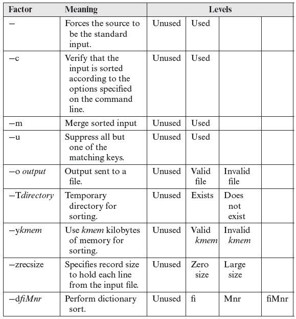
In Tables 6.1 and 6.2, level Unused indicates that the corresponding option is not used while testing the sort command. Used means that the option is used. Level Valid File indicates that the file specified using the -o option exists whereas Invalid file indicates that the specified file does not exist. Other options can be interpreted similarly.
We have identified a total of 20 factors for the sort command. The levels listed in Table 6.1 lead to a total of approximately 1.9 × 10⁹ combinations.
Table 6.2 Factors and levels for the Unix sort utility (continued).
Example 6.5 There is often a need to test a web application on different platforms to ensure that a claim such as “Application X can be used under Windows and OS X.” Here we consider a combination of hardware, operating system, and a browser as a platform. Such testing is commonly referred to as compatibility testing.
Let us identify factors and levels needed in the compatibility testing of application X. Given that we would like X to work on a variety of hardware, OS, and browser combinations, it is easy to obtain three factors, i.e. hardware, OS, and browser. These are listed in the top row of Table 6.3. Notice that instead of listing factors in different rows, we now list them in different columns. The levels for each factor are listed in rows under the corresponding columns. This has been done to simplify the formatting of the table.
Table 6.3 Factors and levels for testing Web application X.
Hardware Operating System Browser Dell Dimension Series
Windows Server 2008-Web Edition
Internet Explorer 9
Apple iMac
Windows Server 2008-R2 standard Edition
Internet Explorer
Apple MacBook Pro
Windows 7 Enterprise
Chrome
OS 10.6
Safari 5.1.6
OS 10.7
Firefox
A quick examination of the factors and levels in Table 6.3 reveals that there are 75 factor combinations. However, some of these combinations are infeasible. For example, OS 10.2 is an OS for the Apple computers and not for the Dell Dimension series PCs. Similarly, the Safari browser is used on Apple computers and not on the PC in the Dell Series. While various editions of the Windows OS can be used on an Apple computer using an OS bridge such as the Virtual PC or Boot Camp, we assume that this is not the case for testing application X.
The discussion above leads to a total of 40 infeasible factor combinations corresponding to the hardware–OS combination and the hardware–browser combination. Thus, in all we are left with 35 platforms on which to test X.
Notice that there is a large number of hardware configurations under the Dell Dimension Series. These configurations are obtained by selecting from a variety of processor types, e.g., Pentium versus Athelon, processor speeds, memory sizes, and several others. One could replace the Dell Dimension Series in Table 6.3 by a few selected configurations. While doing so will lead to more thorough testing of application X, it will also increase the number of factor combinations, and hence the time to test.
Identifying factors and levels allows us to divide the input domain into subdomains, one for each factor combination. The design of test cases can now proceed by selecting at least one test from each subdomain. However, as shown in examples above, the number of subdomains could be too large and hence the need for further reduction. The problem of test case construction and reduction in the number of test cases is considered in the following sections.
6.2 A Combinatorial Test Design Process
Figure 6.1 shows a three-step process for the generation of test cases and test configurations for an application under test. The process begins with a model of the input space if test cases are to be generated. The application environment is modeled when test configurations are to be generated. In either case, the model consists of a set of factors and the corresponding levels. The modeling of input space or the environment is not exclusive and one might apply either one or both depending on the application under test. Examples in the previous section illustrate the modeling process.
Test generation using combinatorial designs can be considered as a three-step process: build a model, generate a combinatorial design, generate tests.
In the second step, the model is input to a combinatorial design procedure to generate a combinatorial object which is simply an array of factors and levels. Such an object is also known as a factor covering design. Each row in this array generates at least one test configuration or one test input. In this chapter, we have described several procedures for generating a combinatorial object. The procedures described make use of Latin squares, orthogonal arrays, mixed orthogonal arrays, covering arrays, and mixed-level covering arrays. While all procedures, and their variants introduced in this chapter are used in software testing, covering arrays, and mixed-level covering arrays seem to be the most useful in this context.
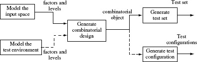
Figure 6.1 A process for generating tests and test configurations using combinatorial designs. A combinatorial design is represented as a combinatorial object which is an array of size N × k with Ν rows, one corresponding to at least one test run and k columns one corresponding to each factor.
A combinatorial object is an array of values, factors and levels. Such an object is also referred to as a factor covering design as the array has at least one occurrence of each value of each factor.
In the final step, the combinatorial object generated is used to design a test set or a test configuration as the requirement might be. The combinatorial object is an array of factor combinations. Each factor combination may lead to one or more test cases where each test case consists of values of input variables and the expected output. However, all combinations generated might not be feasible. Further, the sequence in which test inputs are entered is also not specified in the combinations. The next few examples illustrate how a factor combination may lead to one or more test cases, both feasible and infeasible and assist in detecting errors.
Of the three steps shown in Figure 6.1, the second and third steps can be automated. There are commercial tools available that automate the second step, i.e. the generation of a combinatorial object. Generation of test configurations and test cases requires a simple mapping from integers to levels or values of factors and input variables, a relatively straightforward task.
Example 6.6 From the factor levels listed in Example 6.3, we can generate 75 test cases, one corresponding to each combination. Thus, for example, the next two test inputs are generated from the table in Example 6.3.
Let us assume that the values of File, Edit, and Typeset are set in the sequence listed. Test t1 requires that the tester select “Open” from the File menu, followed by “Paste” from the Edit menu, and finally “Makelndex” from the Typeset menu. While this sequence of test inputs is feasible, i.e. can be applied as desired, the sequence given in t2 cannot be applied.
To test the GUI using t2, one needs to open a “New” file and then use the “Cut” operation from the Edit menu. However, the “Cut” operation is usually not available when a new file is opened, unless there is an error in the implementation. Thus, while t2 is infeasible if the GUI is implemented correctly, it becomes feasible when there is an error in the implementation. While one might consider t2 to be a useless test case, it does provide a useful sequence of input selections from the GUI menus in that it enforces a check for the correctness of certain features.
Example 6.7 Each combination obtained from the levels listed in Table 6.1 can be used to generate many test inputs. For example, consider the combination in which all factors are set to “Unused” except the – o option which is set to “Valid File” and the file option that is set to “Exists.” Assuming that files “afile,” “bfile,” “cfile,” and “dfile” exist, this factor setting can lead to many test cases, two of which are listed below.
< t1 : sort – oafile bfile>
< t2 : sort – ocfile dfile>
One might ask as to why only one of t1 and t2 is not sufficient. Indeed, t2 might differ significantly from t1 in that dfile is a very large sized file relative to bfile. Recall that both bfile and dfile contain data to be sorted. One might want to test sort on a very large file to ensure its correctness and also to measure its performance relative to a smaller data file. Thus, in this example, two tests generated from the same combination are designed to check for correctness and performance.
To summarize, a combination of factor levels is used to generate one or more test cases. For each test case, the sequence in which inputs are to be applied to the program under test must be determined by the tester. Further, the factor combinations do not indicate in any way the sequence in which the generated tests are to be applied to the program under test. This sequence too must be determined by the tester. The sequencing of tests generated by most test generation techniques must be determined by the tester and is not a unique characteristic of tests generated in combinatorial testing.
6.3 Fault Model
The combinatorial design procedures described in this chapter are aimed at generating test inputs and test configurations that might reveal certain types of faults in the application under test. We refer to such faults as interaction faults. We say that an interaction fault is triggered when a certain combination of t ≥ 1 input values causes the program containing the fault to enter an invalid state. Of course, this invalid state must propagate to a point in the program execution where it is observable and hence is said to reveal the fault.
Tests generated using combinatorial designs aim at uncovering interaction faults. Such faults arise due to an interaction of two or more factors.
Faults triggered by some value of an input variable, i.e. t = 1, regardless of the values of other input variables, are known as simple faults. For t = 2, they are known as pairwise interaction faults, and in general, for any arbitrary value of t, as t-way interaction faults. An t–way interaction fault is also known as a t-factor fault. For example, a pairwise interaction fault will be triggered only when two input variables are set to specific values. A 3-way interaction fault will be triggered only when three input variables assume specific values. The next two examples illustrate interaction faults.
A pairwise interaction fault occurs due to an interaction of two factors. A t-way interaction fault occurs due to the interaction of t factors. When t = 1, the fault is considered simple.
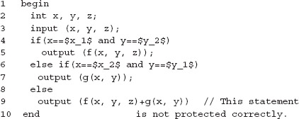
Example 6.8 Consider the following program that requires three inputs x, y, and z. Prior to program execution, variable x is assigned a value from the set {x1, x2, x3},variable y a value from the set {y1, y2, y3}, and variable z a value from the set {z1, z2}. The program outputs the function f(x, y, z) when x = x1 and y = y2, function g(x, y) when x = x2 and y = y1, and function f(x, y, z) + g(x, y), otherwise.
Program P6.1
As marked, Program P6.1 contains one error. The program must output f (x, y, z) – g(x, y) when x = x1 and y = y1 and f(x, y, z) + g(x, y) when x = x2 and y = y2. This error will be revealed by executing the program with x = x1, y = y1, and any value of z, if f (x1, y1, *) – g(x1, y1) ≠ f (x1, y1, *) + g(x1, y1). This error is an example of a pairwise interaction fault revealed only when inputs x and y interact in a certain way. Notice that variable z does not play any role in triggering the fault but it might need to take a specific value for the fault to be revealed (also see Exercises 6.2 and 6.3).
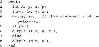
Example 6.9 A missing condition is the cause of a pairwise interaction fault in Program P6.1. Also, the input variables are compared against their respective values in the conditions governing the flow of control. Program P6.2 contains a 3-way interaction fault in which an incorrect arithmetic function of three input variables is responsible for the fault.
Let the three variables assume input values from their respective domains as follows: x ϵ {−1, 1}, y ϵ {−1, 0}, and z ϵ {0, 1}. Notice that there is a total of eight combinations of the three input variables.
Program P6.2
The above program contains a 3-way interaction fault. This fault is triggered by all inputs such that x + y ≠ x – y and z ≠ 0 because for such inputs the program computes an incorrect value of p thereby entering an incorrect state. However, the fault is revealed only by the following two of the eight possible input combinations: x = 1, y = – 1, z = 1 and x = – 1, y = – 1, z = 1.
6.3.1 Fault vectors
As mentioned earlier, a t-way fault is triggered whenever a subset of t ≤ k factors, out of a complete set of k factors, is set to some set of levels. Given a set of k factors f1, f2, . . . , fk, each at qi, 1 ≤ i ≤ k levels, a vector V of factor levels is (l1, l2, . . . , lk), where li, 1 ≤ i ≤ k is a specific level for the corresponding factor. V is also known as a run.
A vector consisting of specific values, or levels, of each factor is known as a run. A run is considered a fault vector if a test derived from it triggers a fault in the IUT.
We say that a run V is a fault vector for program Ρ if the execution of Ρ against a test case derived from V triggers a fault in P. V is considered as a t-way fault vector if any t ≤ k elements in V are needed to trigger a fault in P. Note that a t-way fault vector for Ρ triggers a t-way fault in P. Given k factors, there are k – t don’t care entries in a t-way fault vector. We indicate don’t care entries with an asterisk. For example, the 2-way fault vector (2, 3, ∗) indicates that the 2-way interaction fault is triggered when factor 1 is set to level 2, factor 2 to level 3, and factor 3 is the don’t care factor.
A don’t care entry in a fault vector is indicated by an asterisk (*). It’s value can be set arbitrarily to a factor level and does not affect the fault discovery.
Example 6.10 The input domain of Program P6.2 consists of three factors x, y, and z each having two levels. There is a total of eight runs. For example, (1, 1, 1) and (– 1, – 1, 0) and (– 1, – 1, 0) are two runs. Of these eight runs, (– 1, 1, 1) and (– 1, – 1, 1) are fault vectors that trigger the 3-way fault in Program P6.2. (x1, y1, ∗) is a 2-way fault vector given that the values x1 and y1 trigger the 2-way fault in Program P6.2.
The goal of the test generation techniques described in this chapter is to generate a sufficient number of runs such that tests generated from these runs reveal all t-way faults in the program under test. As we see later in this chapter, the number of such runs increases with the value of t. In many practical situations, t is set to 2 and hence the tests generated are expected to reveal pairwise interaction faults. Of course, while generating t-way runs, one also generates some t + 1, t + 2, . . . , t + k – 1, and k-way runs. Hence, there is always a chance that runs generated with t = 2 reveal some higher level interaction faults.
The aim of the test generation techniques described in this chapter is to generate tests that discover t-way faults. The number of tests generated increase with t.
6.4 Latin Squares
In the previous sections, we have shown how to identify factors and levels in a software application and how to generate test cases from factor combinations. Considering that the number of factor combinations could be exorbitantly large, we want to examine techniques for test generation that focus on only a certain subset of factor combinations.
Latin squares and mutually orthogonal Latin squares are rather ancient devices found useful in selecting a subset of factor combinations from the complete set. In this section, we introduce Latin squares that are used to generate fewer factor combinations than what would be generated by the brute force technique mentioned earlier. Mutually orthogonal Latin squares and the generation of a small set of factor combinations are explained in the subsequent sections.
Let S be a finite set of n symbols. A Latin square of order n is an n × n matrix such that no symbol appears more than once in a row and a column. The term “Latin square” arises from the fact that the early versions used letters from the Latin alphabet A, B, C, and so on in a square arrangement.
A Latin square of order n is an n × n matrix of n-symbols such that no symbol appears more than once in a row or a column.
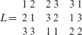
Example 6.11 Given S = {A, B}, here are two Latin squares of order 2.
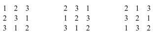
Given S = {1, 2, 3}, we have the following three Latin Squares of order 3.
Additional Latin squares of order 3 can be constructed by permuting rows, columns, and by exchanging symbols, e.g. by replacing all occurrences of symbol 2 by 3 and 3 by 2, of an existing Latin square.
Larger Latin squares of order n can be constructed by creating a row of n distinct symbols. Additional rows can be created by permuting the first row. For example, here is a Latin square Μ of order 4 constructed by cyclically rotating the first row and placing successive rotations in subsequent rows.

Latin squares of a given order n may not be unique. Two Latin squares of order n are considered isomorphic if one can be obtained from the other by a permutation of rows and/or columns and by symbol exchange.
Given a Latin square M, a large number of Latin squares of order 4 can be obtained from Μ through row and column interchange and symbol renaming operations. Two Latin squares M1 and M2 are considered isomorphic if one can be obtained from the other by permutation of rows, columns, and symbol exchange. However, given a Latin square of order n, not all Latin squares of order n can be constructed using the interchange and symbol renaming.
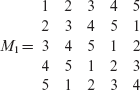
Example 6.12 Consider the following Latin square M1 of order 4.
M1 cannot be obtained from M listed earlier by permutation of rows, columns, or symbol exchange. Exercise 6.6 suggests how M1 can be constructed. Notice that M1 has three 2 × 2 sub-tables that are Latin squares containing the symbol 1. However, there are no such 2 × 2 Latin squares in M.

A Latin square of order n > 2 can also be constructed easily by doing modulo arithmetic. For example, the Latin square Μ of order 4 given below is constructed such that M(i, j) = i + j(mod 4), 1 ≤ i ≤ 4, 1 ≤ j ≤ 4.

A Latin square based on integers 0,1, . . . , n is said to be in standard form if the elements in the top row and the leftmost column are arranged in order. In a Latin square based on letters A, B, and so on, the elements in the top row and the leftmost column are arranged in alphabetical order.
A Latin square is considered to be in standard form if the elements in the top row and the leftmost column are arranged in order.
6.5 Mutually Orthogonal Latin Squares
Let M1 and M2 be two Latin squares, each of order n. Let M1(i, j) and M2(i, j) denote, respectively, the elements in the ith row and jth column of M1 and M2. We now create an n × n matrix M from M1 and M2 such that M(i, j) is M1(i, j)M2(i, j), i.e. we simply juxtapose the corresponding elements of M1 and M2. If each element of M is unique, i.e. it appears exactly once in M , then M1 and M2 are said to be mutually orthogonal Latin squares of order n.
Two Latin squares are considered mutually orthogonal if the matrix obtained by juxtaposing the two has unique elements. Such Latin squares are also referred to as MOLS.
Example 6.13 There are no mutually orthogonal Latin squares of order 2. Listed below are two mutually orthogonal Latin squares of order 3.
To check if indeed M1 and M2 are mutually orthogonal, we juxtapose the corresponding elements to obtain the following matrix.
As each element of M appears exactly once, M1 and M2 are indeed mutually orthogonal.
Mutually orthogonal Latin squares are commonly referred to as MOLS. The term MOLS(n) refers to the set of MOLS of order n. It is known that when n is prime, or a power of prime, MOLS(n) contains n – 1 mutually orthogonal Latin squares. Such a set of MOLS is known as a complete set.
MOLS do not exist for n = 2 and n = 6 but they do exist for all other values of n > 2. Numbers 2 and 6 are known as Eulerian numbers after the famous mathematician Leonhard Euler (1707–1783). The number of MOLS of order n is denoted by N(n). Thus, when n is prime or a power of prime, N(n) = n – 1 (also see Exercise 6.9). The next example illustrates a simple procedure to construct MOLS(n) when n is prime.
There are exactly n – 1 MOLS when n is prime or a power of prime. There are no MOLS for n = 2 and n = 6.
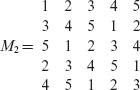
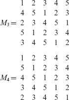
Example 6.14 We follow a simple procedure to construct MOLS(5). We begin by constructing a Latin square of order 5 given the symbol set S = {1, 2, 3, 4, 5}. This can be done by the method described in the previous section, which is to generate subsequent rows of the matrix by rotating the previous row to the left by one position. The first row is a simple enumeration of all symbols in S; the order of enumeration does not matter. Here is one element of MOLS(5)
Next, we obtain M2 by rotating rows 2 through 5 of M1 by two positions to the left.
M3 and M4 are obtained similarly but by rotating the first row of M1 by three and four positions, respectively.
Thus, we get MOLS(5) = {M1, M2, M3, M4}. It is easy to check that indeed the elements of MOLS(5) are mutually orthogonal by superimposing them pairwise. For example, superimposing M2 and M4 leads to the following matrix where each element occurs exactly once.
The method illustrated in the previous example is guaranteed to work only when constructing MOLS(n) for n that is prime or a power of prime. For other values of n, the maximum size of MOLS(n) is n – 1. However, different methods are used to construct MOLS(n) when n is not a prime or a power of prime. Such methods are beyond the scope of this book. There is no general method available to construct the largest possible MOLS(n) for n that is not a prime or a power of prime. The CRC Handbook of Combinatorial Designs (see the Bibliographic Notes section) lists a large set of MOLS for various values of n.
The maximum number of MOLS(n) is n – 1 when n is not prime.
6.6 Pairwise Design: Binary Factors
We now introduce the techniques for selecting a subset of factor combinations from the complete set. First, we focus on programs whose configuration or input space can be modeled as a collection of factors where each factor assumes one or two values. We are interested in selecting a subset from the complete set of factor combinations such that all pairs of factor levels are covered in the selected subset.
A factor is considered binary if it can assume one of the two possible values.
Each factor combination selected will generate at least one test input or test configuration for the program under test. As discussed earlier, the complete set of factor combinations might be too large and impractical to drive a test process, and hence the need for selecting a subset.
To illustrate the process of selecting a subset of combinations from the complete set, suppose that a program to be tested requires three inputs, one corresponding to each input variable. Each variable can take only one of two distinct values. Considering each input variable as a factor, the total number of factor combinations is 23. Let X, Y, and Ζ denote the three input variables and {X1, X2}, {Y1, Y2}, and {Z1, Z2}, their respective sets of values. All possible combinations of these three factors are given below.
(X1, Y1, Z1) (X1, Y1, Z2)
(X1, Y2, Z1) (X1, Y2, Z2)
(X2, Y1, Z1) (X2, Y1, Z2)
(X2, Y2, Z1) (X2, Y2, Z2)
However, we are interested in generating tests such that each pair of input values is covered, i.e. each pair of input values appears in at least one test. There are 12 such pairs, namely (X1, Y1), (X1, Y2), (X1, Z1), (X1, Z2), (X2, Y1), (X2, Y2), (X2, Z1), (X2, Z2), (Y1, Z1), (Y1, Z2), (Y2, Z1), and (Y2, Z2). In this case, the following set of four combinations suffices.
(X1, Y1, Z2) (X1, Y2, Z1)
(X2, Y1, Z1) (X2, Y2, Z2)
The number of tests needed to cover all binary factors is significantly less than what is obtained using exhaustive enumeration.
The above set of four combinations is also known as a pairwise design. Further, it is a balanced design because each value occurs exactly the same number of times. There are several sets of four combinations that cover all 12 pairs (see Exercise 6.8).
Notice that being content with pairwise coverage of the input values reduces the required number of tests from eight to four, a 50% reduction. The large number of combinations resulting from 3-way, 4-way, and higher order designs often force us to be content with pairwise coverage.
Let us now generalize the problem of pairwise design to n ≥ 2 factors where each factor takes on one of two values. To do so, we define S2k–1 to be the set of all binary strings of length 2k – 1 such that each string has exactly k 1s. There are exactly ![]() strings in S2k–1. Recall that
strings in S2k–1. Recall that ![]()
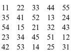
Example 6.15 For k = 2, S3 contains
binary strings of length 3, each containing exactly two 1s. All strings are laid out in the following with column number indicating the position within a string and row number indicating the string count.
For k = 3, S5 contains
binary strings of length 5, each containing three 1s.
Given the number of two-valued parameters, the following procedure can be used to generate a pairwise design. We have named the procedure as the “SAMNA procedure” after its authors (see the Bibliographic Notes section for details).
Procedure for generating pairwise designs.
Input:
n: Number of two-valued input variables (or factors).
Output:
A set of factor combinations such that all pairs of input values are covered.
Procedure:
SAMNA
/*
X1, X2, . . . , Xn denote the n input variables.
denotes one of the two possible values of variable Xi, for 1 ≤ i ≤ n.
One of the two values of each variable corresponds to a 0 and the other to 1.
*/
Step 1
Compute the smallest integer k such that n ≤ |S2k–1|.
Step 2
Select any subset of n strings from S2k–1. Arrange these to form a n × (2k – 1) matrix with one string in each row while the columns contain different bits in each string.
Step 3
Append a column of 0s to the end of each string selected. This will increase the size of each string from 2k – 1 to 2k.
Step 4
Each one of the 2k columns contains a bit pattern from which we generate a combination of factor levels as follows. Each combination is of the kind
where the value of each variable is selected depending on whether the bit in column i, 1 ≤ i ≤ n is a 0 or a 1.
End of procedure SAMNA

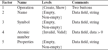
Example 6.16 Consider a simple Java applet named ChemFun that allows a user to create an in-memory database of chemical elements and search for an element. The applet has five inputs listed below with their possible values. We refer to the inputs as factors. For simplicity we have assumed that each input has exactly two possible values.
The applet offers two operations via buttons labeled Create and Show. Pressing the Create button causes the element related data, e.g. its name and atomic number, to be recorded in the database. However, the applet is required to perform simple checks prior to saving the data. The user is notified if the checks fail and data entered is not saved. The Show operation searches for data that matches information typed in any of the four data fields.
Notice that each of the data fields could take on an impractically large number of values. For example, a user could type almost any string using characters on the keyboard in the Atomic number field. However, using equivalence class partitioning, we have reduced the number of data values for which we want to test ChemFun.
Testing ChemFun on all possible parameter combinations would require a total of 25 = 32 tests. However, if we are interested in testing against all pairwise combinations of the five parameters, then only six tests are required. We now show how these six tests are derived using procedure SAMNA.
Given five binary factors (or parameters), exhaustive testing would require 32 tests. However, pairwise testing requires only six tests.
Input:
n = 5 factors.
Output:
A set of factor combinations such that all pairs of input values are covered.
Compute the smallest integer k such that n ≤ |S2k–1|.
In this case we obtain k = 3
Step 2
Select any subset of n strings from S2k–1. Arrange these to form a n × (2k – 1) matrix with one string in each row while the columns contain bits from each string.
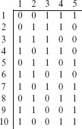
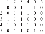
We select first five of the 10 strings in S5 listed in Example 6.15. Arranging them as desired gives us the following matrix.
Step 3
Append 0s to the end of each selected string. This will increase the size of each string from 2k – 1 to 2k.
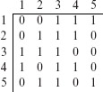
Appending a column of 0s to the matrix above leads to the following 5 × 6 matrix.
Step 4
Each of the 2k columns contains a bit pattern from which we generate a combination of factor values as follows. Each combination is of the kind
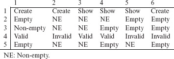
The following factor combinations are obtained by replacing the 0s and 1s in each column of the matrix listed above by the corresponding values of each factor. Here we have assumed that the first of two factor levels listed earlier corresponds to a 0 and the second level corresponds to a 1.
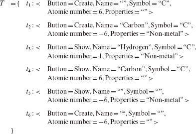
The matrix above lists six factor combinations, one corresponding to each column. Each combination can now be used to generate one or more tests as explained in Section 6.2. The following is a set of six tests for the ChemFun applet.
Each factor combination leads to one test.
The 5 × 6 array of 0s and 1s in Step 2 of Procedure SAMNA, is sometimes referred to as a combinatorial object. While Procedure SAMNA is one method for generating combinatorial objects, several other methods appear in the following sections.
Each method for generating combinatorial objects has its advantages and disadvantages that are often measured in terms of the total number of test cases, or test configurations, generated. In the context of software testing, we are interested in procedures that allow the generation of a small set of test cases or test configurations, while covering all interaction tuples. Usually, we are interested in covering interaction pairs, though in some cases interaction triples or even quadruples might be of interest.
In software testing, we are interested in generating a small set of tests that will likely reveal all t-way interaction faults.
6.7 Pairwise Design: Multi-Valued Factors
Many practical test configurations are constructed from one or more factors where each factor assumes a value from a set containing more than two values. In this section, we show how to use MOLS to construct test configurations when (a) the number of factors is two or more, (b) the number of levels for each factor is more than two, and (c) all factors have the same number of levels.
Next, we list a procedure for generating test configurations in situations where each factor can be at more than two levels. The procedure uses MOLS(n) when the test configuration requires n factors.
Procedure for generating pairwise designs using mutually orthogonal Latin squares.
|
Input: |
n: Number of factors. |
|
Output: |
A set of factor combinations such that all level pairs are covered. |
|
Procedure: |
PDMOLS |
/*
F'1, F'2,..., F'n denote the n factors.
X*i,j denotes the jth level of the ith factor.
*/
|
Step 1 |
Relabel the factors as F1, F2, . . . , Fn such that the following ordering constraint is satisfied: |F1| ≥ |F2| ≥, . . . , ≥ |Fn–1| ≥ |Fn|. Let b=|F1| and k=|F2|. Note that two or more labeling are possible when two or more pairs of factors have the same number of levels. |
|
Step 2 |
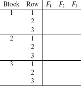
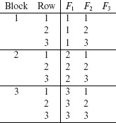
Prepare a table containing n columns and b × k rows divided into b blocks. Label the columns as F1, F2, . . . , Fn. Each block contains k rows. A sample table for n = b = k = 3, when all factors have an equal number of labels, is shown below. |
|
Fill column F1 with 1s in Block 1, 2s in Block 2, and so on. Fill Block 1 of column F2 with the sequence 1, 2, . . . , k in rows 1 through k. Repeat this for the remaining blocks. A sample table with columns 1 and 2 filled is shown below. |
|
Step 4 |
Find s = N(k) MOLS of order k. Denote these MOLS as M1, M2, . . . , Ms. Note that s < k for k > 1. Recall from Section 6.5 that there are at most k – 1 MOLS of order k and the maximum is achieved when k is prime. |
|
Step 5 |
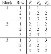
Fill Block 1 of column F3 with entries from column 1 of M1, Block 2 with entries from column 2 of M1, and so on. If the number of blocks b > k, then reuse the columns of M1 to fill rows in the remaining (b – k) blocks. Repeat this procedure and fill columns F4 through Fn using MOLS M2 through Ms. If s < n – 2, then fill the remaining columns by randomly selecting the values of the corresponding factor. Using M1 a sample table for n = k = 3 is shown below. |
|
Step 6 |
The above table lists nine factor combinations, one corresponding to each row. Each combination can now be used to generate one or more tests as explained in Section 6.2. |
In many practical situations, the table of configurations generated using the steps above, will need to be modified to handle constraints on factors and to account for factors that have fewer levels than k. There is no general algorithm for handling such special cases. Examples and exercises in the remainder of this chapter illustrate ways to handle a few situations.
Configurations generated using the algorithm PDMOLS may need to be revised when there are constraints among factors.
The PDMOLS procedure can be used to generate test configurations that ensure the coverage of all pairwise combinations of factor levels. It is easy to check that the number of test configurations so generated is usually much less than all possible combinations. For example, the total number of combinations is 27 for three factors each having three levels. However, as illustrated above, the number of test configurations derived using mutually orthogonal Latin squares is only nine.
For three factors, each having three levels, exhaustive pairwise testing would require 27 tests. However, the PDMOLS procedure can be used to generate only 9 tests that cover all pairwise interactions.
Applications often impose constraints on factors such that certain level combinations are either not possible, or desirable, to achieve in practice. The next, rather long, example illustrates the use of PDMOLS in a more complex situation.
Example 6.17 DNA sequencing is a common activity amongst biologists and other researchers. Several genomics facilities are available that allow a DNA sample to be submitted for sequencing. One such facility is offered by the Applied Genomics Technology Center (AGTC) at the School of Medicine in Wayne State University. The submission of the sample itself is done using a software application available from AGTC. We refer to this software as AGTCS.
AGTCS is supposed to work on a variety of platforms that differ in their hardware and software configurations. Thus, the hardware platform and the operating system are two factors to be considered while developing a test plan for AGTCS. In addition, the user of AGTCS, referred to as Principal Investigator (PI), must either have a profile already created with AGTCS or create a new one prior to submitting a sample. AGTCS supports only a limited set of browsers. In all we have a total of four factors with their respective levels listed below.
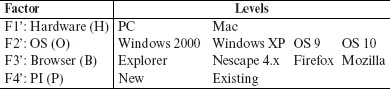
It is obvious that many more levels can be considered for each factor above. However, for the sake of simplicity, we constrain ourselves to the given list.
There are 64 combinations of the factors listed above. However, given the constraint that PCs and Macs will run their dedicated operating systems, the number of combinations reduces to 32, with 16 combinations each corresponding to the PC and the Mac. Note that each combination leads to a test configuration. However, instead of testing AGTCS for all 32 configurations, we are interested in testing under enough configurations so that all possible pairs of factor levels are covered.
We can now proceed to design test configurations in at least two ways. One way is to treat the testing on PC and Mac as two distinct problems and design the test configurations independently. Exercise 6.12 asks you to take this approach and explore its advantages over the second approach used in this example.
The approach used in this example is to arrive at a common set of test configurations that obey the constraint related to the operating systems. Let us now follow a modified version of procedure PDMOLS to generate the test configurations. We use |F| to indicate the number of levels for factor F.
|
Input: |
n = 4 factors. |
|
Output: |
A set of factor combinations such that all pairwise interactions are covered. |
|
Step 1 |
Relabel the factors as F1, F2, F3, and F4 such that |F1| ≥ |F2| ≥ |F3| ≥ |F4|. Doing so gives us F1 = F2′, F2 = F3′, F3 = F1′, and |
|
Step 2 |
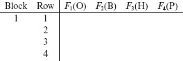
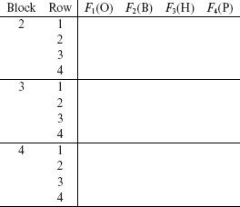
Prepare a table containing 4 columns and b × k = 16 rows divided into four blocks. Label the columns as F1, F2, . . . , Fn. Each block contains k rows. The required table is shown below. |
|
Step 3 |
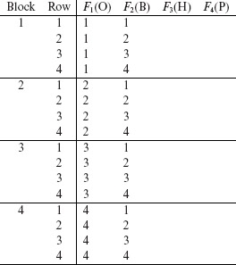
Fill column F1 with 1s in Block 1, 2s in Block 2, and so on. Fill Block 1 of column F2 with the sequence 1, 2, . . . , k in rows 1 through k. Repeat this for the remaining blocks. A sample table with columns F1 and F2 filled is shown below. |
|
Step 4 |
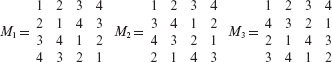
Find MOLS of order 4. As 4 is not prime, we cannot use the procedure described in Example 6.13. In such a situation one may either resort to a predefined set of MOLS of the desired order, or construct ones own using a procedure not described in this book but referred to in the Bibliographic Notes section. We follow the former approach and obtain the following set of three MOLS of order 4. |
|
Step 5 |
Fill the remaining two columns of the table constructed in Step 3. As we have only two more columns to be filled, we use entries from M1 and M2. The final statistical design follows. |
The test configurations constructed in Step 5 do not satisfy the constraints among the factors. Hence, the table needs to be modified.
|
Step 6 |
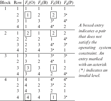
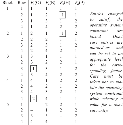
Using the 16 entries in the table above, we can obtain 16 distinct test configurations for AGTCS. However, we need to resolve two problems before we get to the design of test configurations. One problem is that factors F3 and F4 can only assume values 1 and 2, whereas the table above contains other infeasible values for these two factors. These infeasible values are marked with an asterisk (*). |
One simple way to get rid of the infeasible values is to replace them by an arbitrarily selected feasible value for the corresponding factor.
The other problem is that some configurations do not satisfy the operating system constraint. Four such configurations are highlighted in the design above by enclosing the corresponding numbers in rectangles. For example, the entry in Block 3, Row 3 indicates that factor F3, that corresponds to Hardware, is set at level PC while factor F1, that corresponds to Operating System, is set to Mac OS 9.
Obviously, we cannot delete these rows as that would leave some pairs uncovered. For example, removing Block 3, Row 3 will leave the following five pairs uncovered: (F1 = 3, F2 = 3), (F1 = 3, F4 = 2), (F2 = 3, F3 = 1), (F2 = 3, F4 = 2), and (F3 = 1, F4 = 2).
We follow a two step procedure to remove the highlighted configurations and retain complete pairwise coverage. In the first step, we modify the four highlighted rows so they do not violate the constraint. However, by doing so we leave some pairs uncovered. In the second step, we add new configurations that cover the pairs that are left uncovered when we replace the highlighted rows.
Modification of entries in a row might render some pair uncovered. When this happens additional rows will need to be added to the table to ensure complete coverage.
The modified design is as follows. In this design, we have replaced the infeasible entries for factors F3 and F4 by feasible ones (also see Exercise 6.10). Entries changed to resolve conflicts are highlighted. Also, “don’t care” entries are marked with a dash (–). While designing a configuration, a don’t care entry can be selected to create any valid configuration.
It is easy to obtain 20 test configurations from the design given above. Recall that we would get a total of 32 configurations if a brute force method is used. However, by using the PDMOLS procedure, we have been able to achieve a reduction of 12 test configurations. A further reduction can be obtained in the number of test configurations by removing row 2 in block 5 as it is redundant in the presence of row 1 in block 4 (also see Exercise 6.11).
6.7.1 Shortcomings of using MOLS for test design
While the approach of using mutually orthogonal Latin squares to develop test configurations has been used in practice, it has its shortcomings as enumerated below.
While MOLS can be used in the design of combinatorial objects, the process has disadvantages. First, a sufficient number of MOLS of the desired order might not exist, and second the test set so generated is generally larger than what can be obtained using some other methods described later.
- A sufficient number of MOLS might not exist for the problem at hand. As an illustration, in Example 6.17, we needed only two MOLS of order 4 which do exist. However, if the number of factors increases to, say 6, without any change in the value of k=4, then we would be short by one MOLS as there exist only three MOLS of order 4. As mentioned earlier in Step 5 in Procedure PDMOLS, the lack of sufficient MOLS is compensated by randomizing the generation of columns for the remaining factors.
- While the MOLS approach assists with the generation of a balanced design in that all interaction pairs are covered an equal number of times, the number of test configurations is often larger than what can be achieved using other methods.
For example, the application of Procedure PDMOLS to the problem in Example 6.16 leads to a total of nine test cases for testing the GUI. This is in contrast to the six test cases generated by the application of Procedure SAMNA.
Several other methods for generating combinatorial designs have been proposed for use in software testing. The most commonly used are based on the notions of orthogonal arrays, covering arrays, mixed-level covering arrays, and in-parameter order. These methods are described in the following sections.
6.8 Orthogonal Arrays
An orthogonal array is an N × k matrix in which the entries are from a finite set S of s symbols such that any N × t subarray contains each t-tuple exactly the same number of times. Such an orthogonal array is denoted by OA(N, k, s, t). The index of an orthogonal array, denoted by λ, is equal to N/st. N is referred to as the number of runs and t as the strength of the orthogonal array.
An orthogonal array of strength t is an Ν × k array where any Ν × t subarray contains a t-tuple exactly the same number of times. All factors in an orthogonal array have exactly the same number of levels.
When using orthogonal arrays in software testing, each column corresponds to a factor and the elements of a column to the levels for the corresponding factor. Each run, or row of the orthogonal array, leads to a test case or a test configuration. The following example illustrates some properties of simple orthogonal arrays.
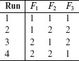
Example 6.18 The following is an orthogonal array having 4 runs and has a strength of 2. It uses symbols from the set {1, 2}. Notationally, this array is denoted as OA(4, 3, 2, 2). Note that the value of parameter k is 3 and hence we have labeled the columns as F1, F2, and F3 to indicate the three factors.
Each row in an orthogonal array is also know as a run.
The index λ of the array shown above is 4/22 = 1 implying that each pair (t = 2) appears exactly once (λ = 1) in any 4 × 2 subarray. There is a total of st = 22 = 4 pairs given as (1, 1), (1, 2), (2, 1), and (2, 2). It is easy to verify, by a mere scanning of the array, that each of the four pairs appears exactly once in each 4 × 2 subarray.
The orthogonal array shown below has 9 runs and a strength of 2. Each of the four factors can be at any one of three levels. This array is denoted as OA(9, 4, 3, 2) and has an index of 1.
There are nine possible pairs of symbols formed from the set {1, 2, 3}. Again, it is easy to verify that each of these pairs occurs exactly once in any 9 × 2 subarray taken out of the matrix given above.
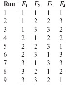
An alternate notation for orthogonal arrays is also used. For example, LN(sk) denotes an orthogonal array of Ν runs where k factors take on any value from a set of s symbols. Here, the strength t is assumed to be 2. Using this notation, the two arrays in Example 6.18 are denoted by L4(23) and L9(33),respectively.
Sometimes a simpler notation LN is used that ignores the remaining three parameters k, s, and t assuming that they can be determined from the context. Using this notation, the two arrays in Example 6.18 are denoted by L4 and L9, respectively. We prefer the notation OA(N, k, s, t).
6.8.1 Mixed-level orthogonal arrays
The orthogonal arrays shown in Example 6.18 are also known as fixed-level orthogonal arrays. This is because the design of such arrays assumes that all factors assume values from the same set of s values. As illustrated in Section 6.1.2, this is not true in many practical situations. In many practical applications, one encounters more than one factor, each taking on a different set of values. Mixed-level orthogonal arrays are useful in designing test configurations for such applications.
A mixed level orthogonal array contains Ν runs of k factors where each factor may have different number of levels.
A mixed-level orthogonal array of strength t is denoted by ![]() indicating N runs where k1 factors are at s1 levels, k2 factors at s2 levels, and so on. The total number of factors is
indicating N runs where k1 factors are at s1 levels, k2 factors at s2 levels, and so on. The total number of factors is ![]()
The formula used for computing the index λ of an orthogonal array does not apply to the mixed-level orthogonal array as the count of values for each factor is a variable. However, the balance property of orthogonal arrays remains intact for mixed-level orthogonal arrays in that any N × t subarray contains each t-tuple corresponding to the t columns, exactly the same number of times, which is λ. The next example shows two mixed-level orthogonal arrays.
Mixed-level orthogonal arrays retain the balance property, i.e., each N × t subarray contains each t-tuple exactly the same number of times.
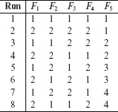
Example 6.19 A mixed-level orthogonal array MA(8, 2441, 2)is shown below. It can be used to design test configurations for an application that contains four factors each at two levels and one factor at four levels.
Notice that the above array is balanced in the sense that in any subarray of size 8 × 2, each possible pair occurs exactly the same number of times. For example, in the two leftmost columns, each pair occurs exactly twice. In columns 1 and 3, each pair also occurs exactly twice. In columns 1 and 5, each pair occurs exactly once.
Mixed-level orthogonal arrays can be used to generate tests when all factors may not have the same number of levels.
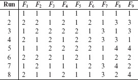
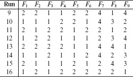
The next example shows MA(16, 2643, 2). This array can be used to generate test configurations when there are six binary factors, labeled F1 through F6 and three factors each with four possible levels, labeled F7 through F9.
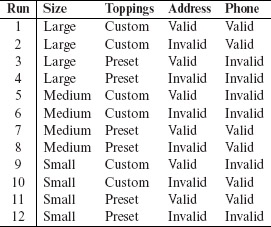
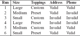
Example 6.20 In Example 6.2, we have three factors at two levels and one factor at three levels. The following mixed array, MA(12, 23, 31, 2) can be used to generate 12 test configurations. This implies that a total of 12 configurations are required for exhaustive testing of the pizza service.
Following is the set of test inputs for the pizza service derived using MA(12, 23, 31, 2) shown above. To arrive at the design below, we assumed that levels 1, 2, and 3 for Size correspond to large, medium, and Small, respectively. Similarly, levels 1 and 2, corresponding to the remaining three factors, are mapped to their respective values in Example 6.2 with a 1 corresponding to the leftmost value and a 2 to the rightmost value. Note that this assignment of integers to actual values is arbitrary and does not affect in any way the generated set of test configurations.
It is easy to check that all possible pairs of factor combinations are covered in the design above. Testing the pizza service under the 12 configurations above will likely reveal any pairwise interaction errors.
So far we have examined techniques for generating balanced combinatorial designs and explained how to use these to generate test configurations and test sets. However, while the balance requirement is often essential in statistical experiments, it is not always so in software testing. For example, if a software application has been tested once for a given pair of factor levels, there is generally no need for testing it again for the same pair, unless the application is known to behave non-deterministically. One might also test the application against the same pair of values to ensure repeatability of results. Thus, for deterministic applications, and when repeatability is not the focus of the test, we can relax the balance requirement and instead use covering arrays, or mixed-level covering arrays for obtaining combinatorial designs. This is the topic of the next section.
While the balance requirement is essential in many statistical experiments, it is not likely to be a requirement in software testing. This observation leads to other techniques for generating tests using combinatorial designs.
6.9 Covering and Mixed-Level Covering Arrays
A covering array CA(N, k, s, t) is an N × k matrix in which entries are from a finite set S of s symbols such that each N × t subarray contains each possible t-tuple at least λ times. As in the case of orthogonal arrays, N denotes the number of runs, k the number factors, s the number of levels for each factor, t the strength, and λ the index. While generating test cases or test configurations for a software application, we use λ = 1.
A covering array is an N × k matrix in which each N × t subarray contains a f-tuple at least a given number of times. In software testing we assume that each N × t aubaray contains each possible t-tuple at least once.
Let us point to a key difference between a covering array and an orthogonal array. While an orthogonal array OA(N, k, s, t) covers each possible t-tuple λ times in any N × t subarray, a covering array CA(N, k, s, t) covers each possible t-tuple at least λ times in any N × t subarray. Thus covering arrays do not meet the balance requirement that is met by orthogonal arrays. This difference leads to combinatorial designs that are often smaller in size than orthogonal arrays. Covering arrays are also referred to as unbalanced designs.
Covering arrays do not meet the balance requirement as different t-tuples in an N × t subarray might occur different number of times. Thus, covering arrays are also known as unbalanced designs.
Of course, we are interested in minimal covering arrays. These are covering arrays that satisfy the requirement of a covering array in the least number of runs.
Example 6.21 A balanced design of strength 2 for 5 binary factors, requires 8 runs and is denoted by OA(8, 5, 2, 2). However, a covering design with the same parameters requires only 6 runs. Thus, in this case, we save two test configurations if we use a covering design instead of the orthogonal array. The two designs follow.
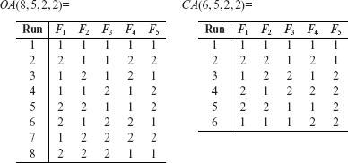
Designs based on covering arrays are generally smaller than those based on orthogonal arrays.
6.9.1 Mixed-level covering arrays
Mixed-level covering arrays are analogous to mixed-level orthogonal arrays in that both are practical designs that allow the use of factors to assume levels from different sets. A mixed-level covering array is denoted as ![]() and refers to an N × Q matrix of entries such that,
and refers to an N × Q matrix of entries such that, ![]() and each N × t subarray contains at least one occurrence of each t-tuple corresponding to the t columns.
and each N × t subarray contains at least one occurrence of each t-tuple corresponding to the t columns.
A mixed-level covering array has factors where each may assume different number of values. Such arrays are generally smaller than mixed-level orthogonal arrays.
Mixed-level covering arrays are generally smaller than mixed-level orthogonal arrays and more appropriate for use in software testing. The next example, shows MCA(6, 2331, 2). Comparing this with MA(12, 2331, 2) from Example 6.20, we notice a reduction of 6 test inputs.
Notice that the array above is not balanced and hence is not a mixed-level orthogonal array. For example, the pair (1, 1) occurs twice in columns Address and Phone but the pair (1, 2) occurs only once in the same two columns. However, this imbalance is unlikely to effect the reliability of the software test process as each of the four possible pairs between Address and Phone are covered and hence will occur in a test input. For the sake of completeness, we list below the set of six tests for the pizza service.
6.10 Arrays of Strength > 2
In the previous sections, we have examined various combinatorial designs all of which have a strength t = 2. While tests generated from such designs are targeted at discovering errors due to pairwise interactions, designs with higher strengths are sometimes needed to achieve higher confidence in the correctness of software. Thus, for example, a design with t = 3 will lead to tests that target errors due to 3-way interactions. Such designs are usually more expensive than designs with t = 2 in terms of the number of tests they generate. The next example illustrates a design with t = 3.
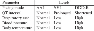
Example 6.22 Pacemakers are medical devices used for automatically correcting abnormal heart conditions. These devices are controlled by software that encodes several complicated algorithms for sensing, computing, and controlling the heart rate. Testing of a typical modern pacemaker is an intense and complex activity. Testing it against a combination of input parameters is one aspect of this activity. The table below lists only five of the several parameters, and their values, that control the operation of a pacemaker.
Due to the high reliability requirement of the pacemaker, we would like to test it to ensure that there are no pairwise or 3-way interaction errors. Thus, we need a suitable combinatorial object with strength 3. We could use an orthogonal array OA(54, 5, 3, 3) that has 54 runs for five factors each at three levels and is of strength 3. Thus, a total of 54 tests will be required to test for all 3-way interactions of the five pacemaker parameters (see also Exercises 6.16 and 6.17).
It is worth noting that a combinatorial array for three or more factors that provides 2-way coverage, balanced or unbalanced, also provides some n-way coverage, for each n > 2. For example, MA(12, 2331, 2) covers all 20 of the 32 3-way interactions of the three binary and one ternary parameters. However, the mixed-level covering array MCA(6, 2331, 2) covers only 12 of the 20 3-way interactions. While (Size=Large, Toppings= Custom, Address=Invalid) is a 3-way interaction covered by MCA (12, 2331, 2), and the triple (Size=Medium, Toppings=Custom, Address=Invalid) is not covered.
A combinatorial array for three or more factors that provides pairwise coverage may also cover some higher order interactions.
6.11 Generating Covering Arrays
Several practical procedures have been developed and implemented for the generation of various types of designs considered in this chapter. Here, we focus on a procedure for generating mixed-level covering arrays for pairwise deigns.
The procedure described below, is known as In-Parameter-Order, or simply IPO, procedure. It takes the number of factors and the corresponding levels as inputs and generates a covering array that is, at best, near optimal. The covering array generated covers all pairs of input parameters at least once and is used for generating tests for pairwise testing. The term “parameter” in “IPO” is a synonym for “factor.”
The IPO procedure has several variants only one of which is presented here. The entire procedure is divided into three parts: the main procedure, named IPO, procedure HG for horizontal growth, and procedure VG for vertical growth. While describing IPO and its sub procedures, we use parameter for factor and value for level.
The In-order-parameter (IPO) procedure is a practical means for constructing mixed-level covering arrays.
Procedure for generating pairwise mixed-level covering designs.
|
Input: |
(a) n ≥ 2: Number of input parameters. (b) Number of values for each parameter. |
|
Output: |
CA: A set of parameter combinations such that all pairs of values are covered at least once. |
|
Procedure: |
IPO |
/*
- F1,F2, . . . ,Fn denote n parameters. q1, q2, . . . , qn denote the number of values for the corresponding parameter.
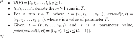
- T holds partial or complete runs of the form (v1, v2, . . . , vk), 1 ≤ k ≤ n, where vi denotes a value for parameter Fi, 1≤ i ≤ k.
- D(F) denotes the domain of parameter F, i.e. the set of all values for parameter F.
*/
The IPO procedure consists of two phases. In the first phase the desire array grows horizontally by the addition of levels to each parameter. In phase two, additional rows are added to the array to include pairs uncovered thus far.
|
Step 1 |
[Initialize] Generate all pairs for parameters F1 and F2. Set T = {(r, s)|for all r ϵ D(F1) and s ϵ D(F2)}. |
|
Step 2 |
[Possible termination] if n=2 then set CA=T and terminate the algorithm, else continue. |
|
Step 3 |
[Add remaining parameters] Repeat the following steps for parameters Fk, k=3, 4, . . . , n. |
End of Procedure IPO
Procedure for horizontal growth.
|
Input: |
(a)T : A set of m ≥ 1 runs of the kind |
|
Output: |
T' : A set of runs (v1, v2, . . . , vk−1, vk), k > 2 obtained by extending the runs in T that cover the maximum number of pairs between parameter Fi, 1 ≤ i ≤ (k–1) and parameter F. |
|
Procedure: |
HG |
|
Step 1 |
Let AP = {(r, s)|,where r is a value of parameter Fi, 1 ≤ i ≤ (k – 1) and s ϵ D(F)}. Thus AP is the set of all pairs formed by combining parameters Fi, 1 ≤ i ≤ (k – 1), taken one at a time, with parameter F. |
|
Step 2 |
Let T'= Ø. T' denotes the set of runs obtained by extending the runs in T in the following steps. |
|
Step 3 |
Let C = min(q,m). Here C is the number of elements in the set T or the set D(F), whichever is less. |
|
Step 4 |
Repeat the next two sub steps for j =1 to C. |
4.1 |
|
4.2 |
|
|
Step 5 |
If C = m, then return T'. |
|
Step 6 |
We will now extend the remaining runs in T by values of parameter F that cover the maximum pairs in AP. Repeat the next four sub steps for j = C +1 to m. |
6.1 |
Let AP' = Ø and v' =l1. |
|
In this step, we find a value of F by which to extend run tj. The value that adds the maximum pairwise coverage is selected. Repeat the next two sub steps for each v ϵ D(F). |
|
6.2.1 |
AP" = {(r, v)|, where r is a value in run tj}. Here AP" is the set of all new pairs formed when run tj is extended by v. |
6.2.2 |
If |AP"| > |AP'|, then AP' = AP" and v' = v. |
6.3 |
Let t'j = extend(tj, v'). T' = T' ∪ t'j. |
6.4 |
AP = AP − AP'. |
|
Step 7 |
Return T'. |
End of Procedure HG
Procedure for vertical growth.
|
Input: |
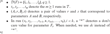
(a)T : A set of m ≥ 1 runs each of the kind (v1, v2, . . . , vk−1, vk), k > 2, where vi, 1 ≤ i ≤ k, is a value of parameter Fi. (b) The set MP of all pairs (r, s), where r is a value of parameter Fi, 1 ≤ i ≤ (k−1), s ϵ D(Fk), and the pair (r, s) is not contained in any run in T. |
| Output: |
A set of runs (v1, v2, . . . , vk−1, vk), k > 2 such that all pairs obtained by combining values of parameter Fi, 1 ≤ i ≤ (k −1) with parameter Fk are covered. |
|
Procedure: |
VG |
|
Step 1 |
Let T' = Ø. |
|
Step 2 |
Add new tests to cover the uncovered pairs. For each missing pair (Fi.r, Fk.s) ϵ MP, 1 ≤ i < k, repeat the next two sub steps. |
2.1 |
If there exists a run (v1, v2 . . . , vi–1, *, vi+1, . . . , vk–1, s) ϵ T', then replace it by the run (v1, v2, . . . , vi–1, r, vi+1, . . . , s) and examine the next missing pair, else go to the next sub step. |
2.2 |
Let t = (dc1, dc2, . . . , dci–1, r, dci+1, . . . , dck–1, s), 1 ≤ i < k. Add t to T'. |
|
For each run t ϵ T', replace any don’t care entry by an arbitrarily selected value of the corresponding parameter. Instead, one could also select a value that maximizes the number of higher order tuples such as triples. |
|
|
Step 4 |
Return T ∪ T'. |
End of Procedure VG
Example 6.23 Suppose it is desired to find a mixed covering design MCA(N, 2132, 2). Let us name the three parameters as A, B, and C, where parameters A and C each have three values and parameter Β has two values. The domains of A, B, and C are, respectively, {a1, a2, a3}, {b1, b2}, and {c1, c2, c3}.
IPO Step 1: Note that n = 3. In this step construct all runs that consist of pairs of values of the first two parameters, A and B. This leads to the following set:
T = {(a1, b1), (a1, b2), (a2, b1), (a2, b2), (a3, b1), (a3, b2)}. We denote the elements of this set, starting from the first element, as t1, t2, . . . , t6.
As n ≠ 2, continue to IPO.Step 3. Execute the loop for k = 3. In the first sub step inside the loop, perform horizontal growth (Step 3.1) using procedure HG. At HG.Step 1, compute the set of all pairs between parameters A and C, and parameters Β and C. This leads us to the following set of 15 pairs.
Next, in HG.Step 2 initialize T' to ∅. At HG.Step 3 compute C = min(q, m) = min(3, 6) = 3. (Do not confuse this C with the parameter C.) Now move to HG.Step 4 where the extension of the runs in T begins ith j = 1.
HG.Step 4.1:
= extend(t1, l1) = (a1, b1, c1). T' = {(a1, b1, c1)}.
HG.Step 4.2: The run just created by extending t1 has covered the pairs (a1, c1) and (b1, c1). Now update AP as follows.
Repeating the above sub steps for j = 2 and j = 3, we obtain the following.
HG.Step 4.1:
= extend(t2, l2) = (a1, b2, c2). T' = {(a1, b1, c1), (a1, b2, c2)}.
HG.Step 4.2:
HG.Step 4.1:
= extend(t3, l3) = (a2, b1, c3). T' = {(a1, b1, c1), (a1, b2, c2), (a2, b1, c3)}.
HG.Step 4.2:
At HG.Step 5 C ≠ 6 and hence continue at HG.Step 6. Repeat the sub steps for j = 4, 5, and 6. Let us first do it for j = 4.
HG.Step 6.1: AP' = Ø and v' = c1. Next, move to HG.Step 6.2. In this step find the best value of parameter C for extending run tj. This step is to be repeated for each value of parameter C. Let us begin with v = c1.
HG.Step 6.2.1: If run t4 by v were to be extended, we get t (a2, b2, c1). This run covers two pairs in AP, namely (a2, c1) and (b2, c1). Hence, AP" = {(a2, c1), (b2, c1)}.
HG.Step 6.2.2: As |AP"| > |AP'|, set AP' ={(a2, c1), (b2, c1)} and v' = c1. Next repeat the two sub steps 6.2.1 and 6.2.2 for v = c2 and then v = c3.
HG.Step 6.2.1: Extending t4 by v = c2, we get the run (a2, b2, c2). This extended run leads to one pair in AP. Hence AP" = {(a2, c2)}.
HG.Step 6.2.2: As |AP"| < |AP'|, do not change AP'.
HG.Step 6.2.1: Now extending t4 by v = c3, we get the run (a2, b2, c3). This extended run gives us (b2, c3) in AP. Hence, AP" = {(b2, c3)}.
HG.Step 6.2.2: As |AP"| < |AP"|, do not change AP'. This completes the execution of the inner loop. We have found that the best way to extend t4 is to do so by c1.
HG.Step 6.3:
= extend(t4, c1) = (a2, b2, c1).
HG.Step 6.4: Update AP by removing the pairs covered by
Let us move to the case j = 5 and find the best value of parameter C to extend t5.
HG.Step 6.1: AP' = Ø, v' = c1, and v = c1.
HG.Step 6.2.1: If run t5 by v were to be extended, we get the run (a3, b1, c1). This run covers one pair in the updated AP, namely (a3, c1). Hence, AP" = {(a3, c1)}.
HG.Step 6.2.2: As |AP"| > |AP'|, set AP' = {(a3, c1)} and v' = c1.
HG.Step 6.2.1: Extending t5 by v = c2 leads to the run (a3, b1, c2). This extended run gives us two pairs, (a3, c2) and (b1, c2) in the updated AP. Hence AP" = {(a3, c2), (b1, c2)}.
HG.Step 6.2.2: As |AP"| > |AP'|, AP' = {(a3, c2), (b1, c2)} and v' = c2.
HG.Step 6.2.1: Next, extend t5 by v = c3, and get (a3, b1, c3). This extended run gives the pair (a3, c3) in AP. Hence, AP" = {(a3, c3)}.
HG.Step 6.2.2: As |AP"| < |AP'|, do not change AP' = {(a3, c2), (b1, c2)}. This completes the execution of the inner loop. We have found that the best way to extend t5 is to do so by c2. Notice that this is not the only best way to extend t5.
HG.Step 6.3:
= extend(t5, c2) = (a3, b1, c2).
HG.Step 6.4: Update AP by removing the pairs covered by
Finally, we move to the last iteration of the outer loop in HG, execute it for j = 6, and find the best value of parameter C to extend t6.
HG.Step 6.1: AP' = Ø, v' = c1, and v = c1.
HG.Step 6.2.1: If run t6 by v were to be extended, we get the run (a3, b2, c1). This run covers one pair in the updated AP, namely (a3, c1). Hence, AP" = {(a3, c1)}.
HG.Step 6.2.2: As |AP"| > |AP'|, set AP' = {(a3, c1)} and v' = c1.
HG.Step 6.2.1: Extending t6 by v = c2, we get the run (a3, b2, c2). This extended run gives us no pair in the updated AP. Hence AP" = Ø.
HG.Step 6.2.2: As |AP"| < |AP'|, AP' and v' remain unchanged.
HG.Step 6.2.1: Next, extend t6 by v = c3, and get (a3, b2, c3). This extended run gives two pairs, (a3, c3) and (b2, c3) in AP. Hence, AP" = {(a3, c3), (b2, c3)}.
HG.Step 6.2.2: As |AP"| > |AP'|, we set AP' = {(a3, c3), (b2, c3)} and v' = c3. This completes the execution of the inner loop. We have found that c3 is the best value of C to extend t6.
HG.Step 6.3:
= extend(t6, c3)=(a3, b2, c3).
HG.Step 6.4: Update AP by removing the pairs covered by
HG.Step 7: We return to the main IPO procedure with Τ' containing six runs.
IPO.Step 3.2: The set of runs T is now the same as the set T' computed in procedure HG. The set of uncovered pairs U is {(a1, c3), (a2, c2), (a3, c1)}. We now move to procedure VG for vertical growth.
IPO.Step 3.3: For each uncovered pair in U, we need to add runs to T.
VG.Step 1: We have m = 6, F = C, D(F) = {c1, c2, c3}, MP = U, and T' = Ø. Recall that m is the number of runs in T', F denotes the parameter to be used for vertical growth, and MP the set of missing pairs.
VG.Step 2:We will consider each missing pair in MP and repeat the sub steps. Begin with the pair (A.a1, C.c3).
VG.Step 2.1: As T' is empty, hence move to the next step.
VG.Step 2.2: t = (a1, *, c3). T' = {(a1, *, c3)}.
VG.Step 2: Next missing pair: {(A.a2, C.c2)}.
VG.Step 2.1: No run in T' is of the kind (*, dc, c2).
VG.Step 2.2: t = (a2, *, c2). T' = {(a1, *, c3), (a2, *, c2)}.
VG.Step 2: Next missing pair: {(A.a3,C.c1)}.
VG.Step 2.1: No run in T' is of the kind (*, dc, c1).
VG.Step 2.2: t = (a3, *, c1). T' = {(a1, *, c3), (a2, *, c2), (a3, *, c1)}. We are done with Step 2.
VG.Step 3: Replace the don’t cares in T' and to obtain the following.
VG.Step 4: Return to procedure IPO with the following set of runs
This loop is now terminated as there are no more parameters to be processed. The desired covering array, namely MCA(9, 2132, 2), is listed below in row–column format. We have replaced ai and ci by i, 1 ≤ i ≤ 3 and bi by i, 1 ≤ i ≤ 2. Parameters A, B, and C are labeled as F1,F2, and F3, respectively.
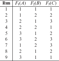
That completes our presentation of an algorithm to generate covering arrays. A detailed analysis of the algorithm has been given by its authors (see the Bibliographic Notes section). To be of any practical use, procedure IPO needs several modifications. Exercise 6.23 lists various types of constraints that are often found in practice and asks you to implement a revised version of procedure IPO.
6.12 Tools
Tool: AETG
Link: http://aetgweb.argreenhouse.com/
Description
Several commercial and free tools are available for the generation of combinatorial designs. AETG was one of the early tools developed at Bellcore (later Telcordia) and remained as the foremost tool in this area. Subsequently, NIST and Professor Jeff Y. Lei from the University of Texas at Arlington developed another tool named ACTS. This tool is available freely from NIST.
The Automatic Efficient Testcase Generator (AETG) was developed at Telcordia Technologies (now Applied Communications Sciences). It is as an online test generation service and can be used to generate t-way test configurations for a variety of factor mix. A formal language can be used to specify constraints among factors. While AETG is a commercial tool, its developers have been liberal in offering free short term access for student training.
Tool: ACTS
Link: http://csrc.nist.gov/groups/SNS/acts/documents/comparison-report.xhtml
Description
ACTS is another freely available tool for generating test configurations. It was developed by Jeff Lie’s group in collaboration with NIST. It is available from NIST as a free download. ACTS is a standalone Java application. It can be used from command line or through a simple GUI. It offers several variations of the IPO algorithm described in this chapter to generate test configurations.
SUMMARY
This chapter has covered a well known set of techniques for the generation of tests for software applications. These techniques fall under the general umbrella of model-based testing and assist with the generation of tests using combinatorial designs. The primary goal of these techniques is to allow the selection of a small number of tests, or test configurations, from a potentially huge test input, or test configuration, domain. While this is also the goal of techniques such as equivalence partitioning and boundary value analysis, test generation based on combinatorial designs is a more formal, and often complementary, discipline.
The combinatorial designs covered in this chapter include orthogonal arrays, mixed orthogonal arrays, covering arrays, and mixed-level covering arrays. In addition, we have explained how to generate tests using mutually orthogonal Latin squares. Mixed-level covering arrays seem to be the most popular choice of combinatorial designs amongst software testers. While there exist several tools and methods for the generation of such designs, we have chosen to describe the In-Parameter Order procedure due to its effectiveness in generating near-minimal mixed-level covering designs and simplicity. Several exercises, and a term project, at the end of this chapter are designed to help you to test and further sharpen your understanding of combinatorial design-based software testing.
Exercises
6.1 When and why would an infeasible test case be useful?
6.2 Program P6.1 contains two if statements. As explained in Example 6.8, this program contains an interaction fault. Consider a test set Τ that ensures that each of the two if statements is executed at least once and that each of the two conditions (x == x1 and y == y2) and (x == x2 and y == y1) evaluates to true and false in some execution on an input from T. (a) Does there exist a test T which will not reveal the interaction fault? (b) Why might the value of z cause the fault to be not revealed even when the fault is triggered?
6.3 Construct an example program that contains one 2-way and one 3-way interaction fault. Generate a test set Τ that reveals the two interaction faults. Specify any conditions that must be satisfied for Τ to be able to reveal the faults.
6.4 A set X is known as a quasigroup under a binary operation op if (a) op is defined on the elements of X, (b) there exist unique elements x, y ϵ X such that for all a, b ϵ X , a op x = b and y op a = b. Prove that the multiplication table for a quasigroup is a Latin Square. (For answer see pages 16–17 in [142].)
6.5 Construct a multiplication table of non-zero integers modulo 5. For example, in your table, 2 × 4 = 3. (a) Is the table you constructed a Latin square? Of what order? (b) Can you generalize this method to construct a Latin square of any order n > 2?
6.6 Construct a 4 × 4 addition table of binary 2-bit strings modulo 2. For example, 01 + 11 = 10 and 11 + 11 = 00. Replace each element in the table by its decimal equivalent plus 1. For example, 11 is replaced by 4. Is the resulting table a Latin square? Generalize this method for constructing Latin squares of order n.
6.7 Construct MOLS(7) given ![]() . (Note: You may have guessed that it is easier to write a computer program to construct MOLS(n) when n is a prime or a power of prime than to do so by hand, especially for larger values of n.)
. (Note: You may have guessed that it is easier to write a computer program to construct MOLS(n) when n is a prime or a power of prime than to do so by hand, especially for larger values of n.)
6.8 Given three two-valued factors X, Y, and Z, list all minimal sets of factor combinations that cover all pairs of values.
6.9 Let N(n) denote the maximum number of mutually orthogonal Latin squares. What is N(k) for K = 1,2,3?
6.10 In Example 6.17, we modified the design generated using MOLS so as to satisfy the operating system constraint. However, we did so by altering the values in specific entries so that all pairs are covered. Suggest other ways to resolving the infeasible values when using MOLS to generate test configurations. Discuss advantages and disadvantages of the ways you suggest.
6.11 Example 6.17 illustrates how to obtain a statistical design that covers all interaction pairs in 20 configurations instead of 32.
- Enumerate all test configurations by listing the levels for each factor.
- How many interactions pairs are covered more than once?
- Derive an alternate design that covers all interaction pairs and satisfies the operating system and hardware related constraint.
- Is your design better than the design in Example 6.17 in any way?
- Can you think of any error in the AGTCS software that might not be discovered by testing against the 20 configurations derived in Example 6.17?
6.12 This exercise is intended to show how constraints on factors could lead to the partitioning of the test configuration problem into two or more simpler problems that are solved independently using the same algorithm.
- Design test configurations for testing the AGTCS application described in Example 6.17. Use the PDMOLS procedure to arrive at two sets of test configurations, one for the PC and the other for the Mac. Note that the PDMOLS procedure is to be applied on two sets of factors, one related to the PC and the other to the Mac.
- Compare the test configurations derived in (a) with those derived in Example 6.17 in terms of their impact on the test process for AGTCS.
6.13 How many test cases will be generated if the PDMOLS procedure is applied to the GUI problem in Example 6.16?
6.14 Given three factors x ϵ {–1, 1}, y ϵ {–1, 1}, and z ϵ {0, 1}, construct an orthogonal array OA(N, 3, 2, 2). (a) Using the array you have constructed, derive a set of Ν tests for the program in Example 6.9. (b) Which of the Ν tests triggers the fault in Program P6.2? (c) What conditions must be satisfied for the fault to be revealed, i.e. propagate to the output of the program? (d) Construct, if possible, non-trivial functions f and g that will prevent the triggered fault to propagate to the output.
6.15 Consider an application iAPP intended to be used from any of three different browsers (Safari, Internet Explorer, and Firefox) running on three operating systems (Windows, Mac OS, and Linux). The application must be able to connect to other devices using any of three connection protocols (LAN, PPP, and ISDN). The application must also be able to send output to a printer that is networked or local, or to the screen.
- Identify the factors and levels in the problem mentioned above.
- Use Procedure PDMOLS to generate test configurations for iAPP.
6.16 Example 6.22 suggests the use of OA(54, 5, 3, 3) to cover all 3-way interactions. Look up this array on the Internet and design all 54 tests for the pacemaker. Refer to the “CRC Handbook of Combinatorial Design” cited in the Bibliographic Notes section. How many tests are required if the coverage requirement is relaxed to pairwise coverage?
6.17 As indicated in Example 6.22, a total of 54 tests are required to cover all 3-way interactions. (a) What is the minimum number of tests required to test for all 3-way interactions given five parameters each assuming one of three values. (b) Design a minimal covering array CA(N, 5, 3, 3), where Ν is the number of runs needed.
6.18 A complete factorial array of Q factors is a combinatorial object that contains all possible combinations of Q factors. In some cases, a combinatorial array is a minimal size array of a given strength and index. Which of the following arrays is complete factorial? (We have not specified the number of runs. For answers, refer to the handbook mentioned in Exercise 6.16.)
- MA(N, 3151, 2)
- OA(N, 4, 3, 2)
- MA(N, 2131, 2)
- OA(N, 5, 2, 4)
6.19 Justify the name “In-Parameter-Order” for procedure IPO.
6.20 Is MCA(10, 2132, 2) generated in Example 6.23 using procedure IPO, a minimal array? Is this a mixed orthogonal array?
6.21 In Example 6.23, we assumed F1 = A, F2 = B, and F3 = C. Would the size of the resulting array be different if we were to use the assignment F1 = A, F2 = C, and F3 = B?
6.22 (a) At Step 3 of procedure VG, we can replace the don’t care values to maximize the number of higher order tuples. Can you replace the don’t care values in Example 6.23, VG.Step 3, so that the number of triples covered is more than the number covered in the array on page 341? (b) What is the minimum array size needed to cover all possible triples of factors A, B, and C?
- Consider the following types of constraints that might exist in a software test environment. Prohibited pairs
A set of pairs that must not appear in the covering array.
Prohibited higher order tuples
A set of n-order tuples, n > 2, must not appear in a covering array of strength 2.
Factor coupling
If factor A is set to r then factor Β must be set to s, where r and s belong to, respectively, D(A) and D(B). This relationship can be generalized to the following.
If X(F1, F2, . . . , Fn) then Y1, Y2, . . . , Ym; n, m ≥ 1.
where X is a relation amongst one or more factors and Ys are constraints on factors. For example, a simple relation exists when X ϵ {<, ≤, =, >, ≥, ≠}. Such relations might also exist among more than two factors.
Procedure IPO does not consider any factor related constraints while generating a covering design. Rewrite IPO by including the ability to input and satisfy the constraints listed above. You might solve this problem in an incremental fashion. For example, you might start with modifying IPO so that only the Prohibited pairs constraint is included. Then proceed to include the other constraints incrementally.
- Think of some practical relations that correspond to X above. Include these in the revised IPO.
- Write a Java applet that implements the revised IPO procedure.
- If you want to, commercialize your applet and make some money by selling it! watch out for companies that have patented algorithms for the generation of combinatorial designs.