5.5  Characterization Set

Most methods for generating tests from FSMs make use of an important set known as the characterization set. This set is usually denoted by W and is sometimes referred to as the W-set. In this section, we explain how one can derive a W-set, given the description of an FSM. Let us examine the definition of the W-set.

 

Let Μ = (X, Y, Q, q₁, δ, O) be an FSM that is minimal and complete. A characterization set for M, denoted as W, is a finite set of input sequences that distinguish the behavior of any pair of states in M. Thus, if q_i and q_j are states in Q, then there exists a string s in W such that O(s, q_i) ≠ O(s, q_j), where s belongs to X⁺.

 

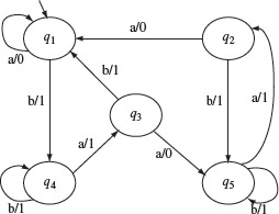
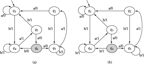
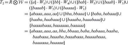
Example 5.7   Consider an FSM M = (X, Y, Q, q₁, δ, O) where X = {a, b}, Y = {0, 1}, and Q = {q₁, q₂, q₃, q₄, q₅}, q₁ is the initial state. The state transition function δ and the output function Ο are shown in Figure 5.13. The set W for this FSM is given below.

 

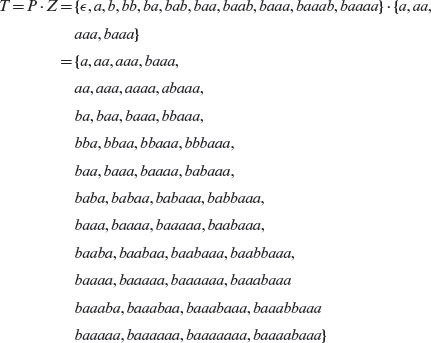
W = {a, aa, aaa, baaa}

  

A distinguishing sequence x for two states r and s of an FSM Μ causes Μ to produce different outputs when excited by x starting in states r or in s.

Let us do a sample check to determine if indeed, W is the characterization set for M. Consider the string baaa. It is easy to verify from Figure 5.13 that when Μ is started in state q₁ and excited with baaa, the output sequence generated is 1101. However, when Μ is started in state q₂ and excited with input baaa, the output sequence generated is 1100. Thus, we see that O(baaa, q₁) ≠ O(baaa, q₂) implying that the sequence baaa is a distinguishing sequence for states q₁ and q₂. You may now go ahead and perform similar checks for the remaining pairs of states.

Figure 5.13 The transition and output functions of a simple FSM.

The algorithm to construct a characterization set for an FSM Μ consists of two main steps. The first step is to construct a sequence of k-equivalence partitions P₁, P₂, . . . , P_m where m > 0. This iterative step converges in at most n steps where n is the number of states in M. In the second step, these k-equivalence partitions are traversed, in reverse order, to obtain the distinguishing sequences for every pair of states. These two steps are explained in detail in the following two subsections.

5.5.1  Construction of the k-equivalence partitions

Recall that given Μ = (X, Y, Q, q₁, δ, O), two states q₁ ϵ Q and q_j ϵ Q are considered k-equivalent, if there does not exist an s ϵ X^k such that O(s, q_i) ≠ O(s, q_j). The notion of k-equivalence leads to the notion of k-equivalence partitions.

 

Given an FSM Μ = (X, Y, Q, q₁, δ, O), a k-equivalence partition of Q, denoted by P_k, is a collection of n finite sets of states denoted as Σ_{k 1}, Σ_{k 2}, . . . , Σ_kn such that

• 
• States in Σ_kj , for 1 ≤ j ≤ n, are k-equivalent,
• If q_l ϵ Σ_ki and q_m ϵ Σ_kj, for i ≠ j, then q_l and q_m must be k-distinguishable.

We now illustrate the computation of k-equivalence partitions by computing them for the FSM of Example 5.7 using a rather long example.

 

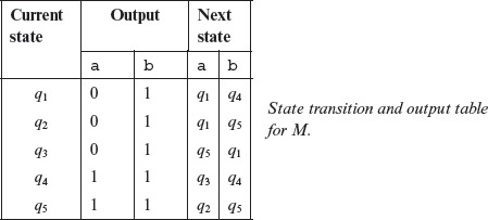
Example 5.8   We begin by computing the 1-equivalence partition, i.e. P₁, for the FSM shown in Figure 5.13. To do so, write the transition and output functions for this FSM in a tabular form as shown below.

The next step in constructing P₁ is to regroup the states so that all states that are identical in their output entries belong to the same group. Separation among two groups is indicated by a horizontal line as shown in the table below. Note from this table that states q₁, q₂, and q₃ belong to one group as they share identical output entries. Similarly, states q₄ and q₅ belong to another group. Notice also that we have added a Σ column to indicate group names. You may decide on any naming scheme for groups. In this example, groups are labeled as 1 and 2.

The construction of P₁ is now complete. The groups separated by the horizontal line constitute a 1-equivalence partition. We have labeled these groups as 1 and 2. Thus, we get the 1-equivalence partition as

P₁ = {1, 2}

Group 1 = Σ₁₁ = {q₁, q₂, q₃}

Group 2 = Σ₁₂ = {q₄, q₅}

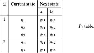
In preparation to begin the construction of the 2-equivalence partition, construct the P₁ table as follows. First, we copy the “Next State” sub-table. Next, rename each Next State entry by appending a second subscript which indicates the group to which that state belongs. For example, the next state entry under column “a” in the first row is q₁. As q₁ belongs to group 1, we relabel this as q₁₁. Other next state entries are relabeled in a similar way. This gives us the P₁ table as shown below.

 

Each P-table contains two or more groups of states. Each group of states is k-equivalent for some k > 0.

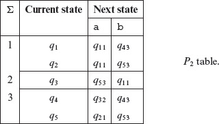
From the P₁ table given above, construct the P₂ table as follows. First, regroup all rows with identical second subscripts in its row entries under the Next State column. Note that the subscript we are referring to is the group label. Thus, for example, in q₄₂ the subscript we refer to is 2 and not 4 2. This is because q₄ is the name of the state in machine Μ and 2 is the group label under the Σ column. As an example of regrouping in the P₁ table, the rows corresponding to the current states q₁ and q₂ have next states with identical subscripts and hence we group them together. This regrouping leads to additional groups. Next, relabel the groups and update the subscripts associated with the next state entries. Using this grouping scheme, we get the following P₂ table.

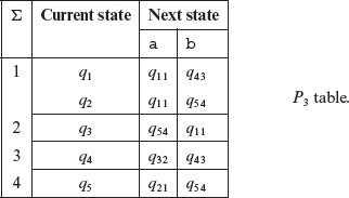
Notice that there are three groups in the P₂ table. Regroup the entries in the P₂ table using the scheme described earlier for generating the P₂ table. This regrouping and relabeling gives us the following P₃ table.

Further regrouping and relabeling of P₃ table gives us the P₄ table given below.

Note that no further partitioning is possible using the scheme described earlier. We have completed the construction of k-equivalence partitions, k = 1,2,3,4, for machine M.

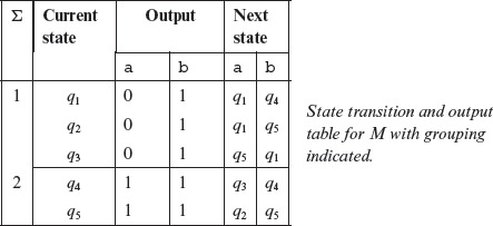
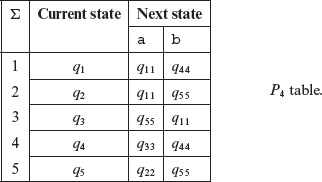
Notice that the process of deriving the P_k tables converged to P₄ and no further partitions are possible. See Exercise 5.6 that asks you to show that indeed the process will always converge. It is also interesting to note that each group in the P₄ table consists of exactly one state. This implies that all states in Μ are distinguishable. In other words, no two states in Μ are equivalent.

Let us now summarize the algorithm to construct a characterization set from the k-equivalence partitions and illustrate it using an example.

5.5.2  Deriving the characterization set

Having constructed the k-equivalence partitions, i.e. the P_k tables, we are now ready to derive the W-set for machine M. Recall that for each pair of states q_i and q_j in M, there exists at least one string in W that distinguishes q_i from q_j. Thus, the method to derive W proceeds by determining a distinguishing sequence for each pair of states in M. First, we sketch the method, referred to as the W procedure, and then illustrate it by a continuation of the previous example. In the procedure below, G(q_i, x) denotes the label of the group to which an FSM moves when excited using input x in state q_i. For example, in the table for P₃, G(q₂, b) = 4 and G(q₅, a) = 1.

 

The W-Procedure to derive W from a set of partition tables.

1. Let M = (X, Y, Q, q₁, δ, O) be the FSM for which P = {P₁, P₂, . . . , P_n} is the set of k-equivalence partition tables for k = 1,2, . . . , n. Initialize W = Ø.
2. Repeat the steps (a) through (d) for each pair of states (q_i, q_j), i ≠ j, in M.
   1. Find an r, 1 ≤ r < n such that the states in pair (q_i, q_j) belong to the same group in P_r but not in P_r+1. In other words, P_r is the last of the P tables in which (q_i, q_j) belong to the same group. If such an r is found, then move to Step (b), otherwise find an η ϵ X such that O(q_i, η) ≠ O(q_j, η), set W = W ∪ {η}, and continue with the next available pair of states.
      

      The length of the minimal distinguishing sequence for (q_i, q_j) is r + 1.

      Denote this sequence as z = x₀x₁ . . . x_r where x_i ϵ X for 0 ≤ i ≤ r.

   2. Initialize z = ϵ. Let p₁ = q_i and p₂ = q_j be the current pair of states. Execute steps (i) through (iii) for m = r, r – 1, r – 2, . . . , 1.
      1. Find an input symbol η in P_m such that G(p₁, η) ≠ G(p₂, η). In case there is more than one symbol that satisfies the condition in this step, then select one arbitrarily.
      2. Set z = z.η.
      3. Set p₁ = δ(p₁, η) and p₂ = δ(p₂, η).
   3. Find an η ϵ X such that O(p₁, η) ≠ O(p₂, η). Set z = z.η.
   4. The distinguishing sequence for the pair (q_i, q_j) is the sequence z. Set W = W ∪ {z}.

Upon termination of the W procedure, we would have generated distinguishing sequences for all pairs of states in M. Note that the above algorithm is inefficient in that it derives a distinguishing sequence for each pair of states even though two pairs of states might share the same distinguishing sequence. (See Exercise 5.7.) The next example applies the W procedure to obtain W for the FSM in Example 5.8.

 

Example 5.9   As there are several pairs of states in M, we illustrate how to find the distinguishing input sequences for the pairs (q₁, q₂) and (q₃, q₄). Let us begin with the pair (q₁, q₂).

According to Step 2(a) of the W procedure, we first determine r. To do so, note from Example 5.8 that the last P-table in which q₁ and q₂ appear in the same group is P₃. Thus r = 3.

Next, we move to Step 2(b) and set z = ϵ, p₁ = q₁, p₂ = q₂. From P₃, we find that G(p₁, b) ≠ G(p₂, b) and update z to z = zb. Thus, b is the first symbol in the input string that distinguishes q₁ from q₂. In accordance with Step 2(b)(iii), reset p₁ = δ(p₁, b) and p₂ = δ(p₂, b). This gives us p₁ =q₄ and p₂ = q₅.

Going back to Step 2(b)(i), we find from the P₂ table that G(p₁, a) ≠ G(p₂, a). Update z to z.a = ba and reset p₁ and p₂ to p₁ = δ(p₁, a) and p₂ = δ(p₂, a). We now have p₁ = q₃ and p₂ = q₂. Hence, a is the second symbol in the string that distinguishes states q₁ and q₂.

Once again return to Step 2(b)(i). We now focus our attention on the P₁ table and find that states G(p₁, a) ≠ G(p₂, a) and also G(p₁, b) ≠ G(p₂, b). We arbitrarily select a as the third symbol of the string that will distinguish states q₃ and q₂. In accordance with Steps 2(b)(ii) and 2(b)(iii), z, p₁, and p₂ are updated as z = z.a = baa, P₁ = δ(p₁, a) and p₂ = δ(p₂, a). This update leads to p₁ = q₅ and P₂ = q₁.

Finally at Step 2(c), the focus is on the original state transition table for M. States q₁ and q₅ in the table are distinguished by the symbol a. This is the last symbol in the string to distinguish states q₁ and q₂. Next, set z = z.a = baaa. The string baaa is now discovered as the input sequence that distinguishes states q₁ and q₂. This sequence is added to W. Note from Example 5.7 that indeed baaa is a distinguishing sequence for states q₁ and q₂.

Next, the pair (q₃, q₄) is selected and the procedure resumes at Step 2(a). These two states are in a different group in table P₁ but in the same group in M. Thus, r = 0. As O(q₃, a) ≠ O(q₄, a), the distinguishing sequence for the pair (q₃, q₄) is the input sequence a.

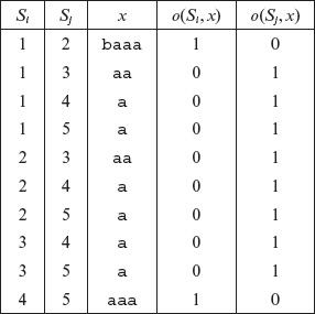
It is left to the reader to derive distinguishing sequences for the remaining pairs of states. A complete set of distinguishing sequences for FSM Μ is given in Table 5.2. The leftmost two columns labeled S_i and S_j contain pairs of states to be distinguished. The column labeled x contains the distinguishing sequence for the pairs of states to its left. The rightmost two columns in this table show the last symbol output when input x is applied to state S_i and S_j, respectively. For example, as we have seen earlier O(q₁, baaa) = 1101. Thus, in Table 5.2, we only show the 1 in the corresponding output column. Notice that each pair in the last two columns is different, i.e. O(S_i, x) ≠ O(S_j, x) in each row. From this table, we obtain W = {a, aa, aaa, baaa}. While the sequence aa can be used instead of using a, doing so would lead to a longer tests.

 

Table 5.2 Distinguishing sequences for all pairs of states in the FSM of Example 5.8.

5.5.3  Identification sets

Consider an FSM Μ = (X, Y, Q, q₁, δ, O) with symbols having their usual meanings and |Q| = n. Assume that Μ is completely specified and minimal. We know that a characterization set W for Μ is a set of strings such that for any pair of states q_i and q_j in M, there exists a string s in W such that O(q_i, s) ≠ (q_j, s).

 

Analogous to the characterization set for M, we associate an identification set with each state of M. An identification set for state q_i ϵ Q is denoted by W_i and has the following properties: (a) W_i ⊆ W, 1 ≤ i ≤ n, (b) O(q_i, s) ≠ O(q_j, s), for any j, 1 ≤ j ≤ n, j ≠ i, s ϵ W_i, and (c) no subset of W_i satisfies property (b). The next example illustrates the derivation of the identification sets given W.

 

Example 5.10    Consider the machine given in Example 5.9 and its characterization set W shown in Table 5.2. From this table, we notice that state q₁ is distinguished from the remaining states by the strings baaa, aa, and a. Thus, W₁ = {baaa, aa, a}. Similarly, W₂ = {baaa, aa, a}, W₃ = {a, aa}, W₄ = {a, aaa}, and W₅ = {a, aaa}.

 

While the characterization sets are used in the W-method, the W_i sets are used in the Wp-method. The W- and the Wp-methods are used for generating tests from an FSM. We are now well equipped to describe various methods for test generation given an FSM. We begin with a description of the W-method.

5.6  The W-method

The W-method is used for constructing a test set from a given FSM M. The test set so constructed is a finite set of sequences that can be input to a program whose control structure is modeled by M. Alternately, the tests can also be the input to a design to test its correctness with respect to some specification.

The implementation modeled by Μ is also known as the Implementation Under Test and abbreviated as IUT. Note that most software systems cannot be modeled accurately using an FSM. However, the global control structure of a software system can be modeled by an FSM. This also implies that the tests generated using the W-method, or any other method based exclusively on a finite state model of an implementation, will likely reveal only certain types of faults. Later in Section 5.9, we discuss what kinds of faults are revealed by the tests generated using the W-method.

 

5.6.1  Assumptions

The W-method makes the following assumptions for it to work effectively.

1. Μ is completely specified, minimal, connected, and deterministic.
2. Μ starts in a fixed initial state.
3. Μ can be reset accurately to the initial state. A nul1 output is generated during the reset operation.
4. Μ and IUT have the same input alphabet.

Later in this section, we examine the impact of violating the above assumptions. Given an FSM M = (X, Y, Q, q₀, δ, O), the W-method consists of the following sequence of steps.

 

Step A	Estimate the maximum number of states in the correct design.
Step B	Construct the characterization set W for the given machine M.
Step C	Construct the testing tree for Μ and determine the transition cover set P.
Step D	Construct set Z.
Step E	Ρ · Ζ is the desired test set.

 

We already know how to construct W for a given FSM. In the remainder of this section, we explain each of the remaining three steps mentioned above.

5.6.2  Maximum number of states

We do not have access to the correct design or the correct implementation of the given specification. Hence, there is a need to estimate the maximum number of states in the correct design. In the worst case, i.e. when no information about the correct design or implementation is available, one might assume that the maximum number of states is the same as the number of states in M. The impact of an incorrect estimate is discussed after we have examined the W-method.

 

5.6.3  Computation of the transition cover set

A transition cover set, denoted as P, is defined as follows. Let q_i and q_j, i ≠ j, be two states in Μ. Ρ consists of sequences sx such that δ(q₀, s) = q_i and δ(q_i, x) = q_j. The empty sequence ϵ is also in P. We can construct Ρ using the “testing tree” of M. A testing tree for an FSM is constructed as follows.

 

1. State q₀, the initial state, is the root of the testing tree.
2. Suppose that the testing tree has been constructed until level k. The (k + 1)^th level is built as follows.
   • Select a node n at level k. If n appears at any level from 1 through k, then n is a leaf node and is not expanded any further. If n is not a leaf node then we expand it by adding a branch from node n to a new node m if δ(n, x) = m for x ϵ X. This branch is labeled as x. This step is repeated for all nodes at level k.

The following example illustrates construction of a testing tree for the machine in Example 5.8 whose transition and output functions are shown in Figure 5.13.

 

Example 5.11   The testing tree is initialized with the initial state q₁ as the root node. This is level 1 of the tree. Next, we note that δ(q₁, a) = q₁ and δ(q₁, b) = q₄. Hence, we create two nodes at the next level and label them as q₁ and q₄. The branches from q₁ to q₁ and q₄ are labeled, respectively, a and b. As q₁ is the only node at level 1, we now proceed to expand the tree from level 2.

At level 2, we first consider the node labeled q₁. However, another node labeled q₁ already appears at level 1, hence this node becomes a leaf node and is not expanded any further. Next, we examine the node labeled q₄. Note that δ(q₄, a) = q₃ and δ(q₄, b) = q₄. We therefore create two new nodes at level 3 and label these as q₄ and q₃ and label the corresponding branches as b and a, respectively.

We proceed in a similar manner down one level in each step. The method converges when at level 6 we have the nodes labeled q₁ and q₅ both of which appear at some level up the tree. We thus arrive at the testing tree for Μ as shown in Figure 5.14.

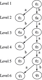
Figure 5.14 Testing tree for the machine with transition and output functions shown in Figure 5.13.

Once a testing tree has been constructed, the transition cover set Ρ is obtained Ρ by concatenating labels of all partial paths along the tree.

 

A partial path is a path starting from the root of the testing tree and terminating in any node of the tree. Traversing all partial paths in the tree shown in Figure 5.14, we obtain the following transition cover set.

It is important to understand the function of the elements of P. As the name transition cover set implies, exciting an FSM in q₀, the initial state, with an element of P, forces the FSM into some state. After the FSM has been excited with all elements of P, each time starting in the initial state, the FSM has reached every state. Thus, exciting an FSM with elements of Ρ ensures that all states are reached, and all transitions have been traversed at least once. For example, when the FSM Μ of Example 5.8 is excited by the input sequence baab in state q₁, it traverses the branches (q₁, q₄), (q₄, q₃), (q₃, q₅), and (q₅, q₅), in that order. The empty input sequence ϵ, does not traverse any branch but is useful in constructing the desired test sequence as is explained next.

 

5.6.4  Constructing Ζ

Given the input alphabet X and the characterization set W, it is straightforward to construct Z. Suppose that the number of states estimated to be in the IUT is m and the number of states in the design specification is n, m ≥ n. Given this information, Ζ can be computed as follows.

Z = (X⁰ · W)∪(X · W)∪(X² · W) . . .∪(X^m−1–n · W)∪(X^m−n · W)

It is easy to see that Z = X · W for m = n, i.e. when the number of states in the IUT is the same as that in the specification. For m < n, we use Z = X · W. Recall that X⁰ = {ϵ}, X¹ = X, X_² = X · X, and so on, where the symbol "·" denotes the string concatenation operation. For convenience, we shall use the shorthand notation X[p] to denote the following set union

{ϵ} ∪ X¹ ∪ X² . . . ∪ X^p–1 ∪X^p.

We can now rewrite Ζ as Ζ = X[m–n]. W, for m≥n where m is the number of states in the IUT and n the number of states in the design specification.

5.6.5  Deriving a test set

Having constructed Ρ and Z, we can easily obtain a test set Τ as Ρ · Ζ. The next example shows how to construct a test set from the FSM of Example 5.8.

 

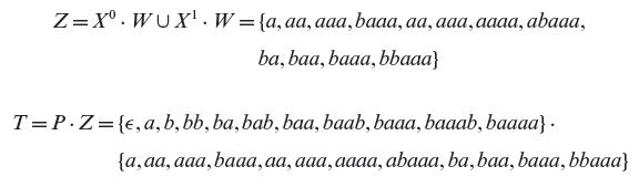
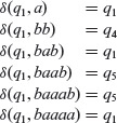
Example 5.12   For the sake of simplicity, let us assume that the number of states in the correct design or IUT is the same as in the given design shown in Figure 5.13. Thus, m = n = 5. This leads to the following Z:

Ζ = X° · W = {a, aa, aaa, baaa}

Catenating Ρ with Z, we obtain the desired test set.

Assuming that the IUT has one extra state, i.e. m = 6, we obtain Ζ and the test set P · Z as follows. 

5.6.6  Testing using the W-method

To test a given IUT Μ_i against its specification M, we do the following for each test input.

1. Find the expected response M(t) to a given test input t. This is done by examining the specification. Alternately, if a tool is available, and the specification is executable, one could determine the expected response automatically.
2. Obtain the response M_i(t) of the IUT, when excited with t in the initial state.
3. If M(t) = M_i(t), then no flaw has been detected so far in the IUT. M(t) ≠ M_i(i) implies the possibility of a flaw in the IUT under test, given a correct design.

Notice that a mismatch between the expected and the actual response does not necessarily imply an error in the IUT. However, if we assume that (a) M(t) and M_i(t) have been determined without any error, and (b) the comparison between M(t) and M_i(t) is correct, then indeed M(t) ≠ M_i(t) implies an error in the design or the IUT.

 

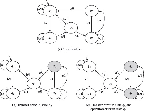
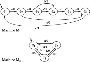
Example 5.13   Let us now apply the W-method to test the design shown in Figure 5.13. We assume that the specification is also given in terms of an FSM which we refer to as the “correct design.” Note that this might not happen in practice but we make this assumption for illustration.

Consider two possible implementations under test. The correct design is shown in Figure 5.15(a) and is referred to as M. We denote the two erroneous designs, corresponding to two IUTs under test, as M₁ and M₂, respectively, shown in Figure 5.15(b) and (c).

Figure 5.15 The transition and output functions of FSMs of the design under test, denoted as Μ in the text and copied from Figure 5.13 and two incorrect designs in (b) and (c) denoted as M₁, and M₂ in the text.

Notice that M₁ has one transfer error with respect to M. The error occurs in state q₂ where the state transition on input a should be δ₁(q₂, a) = q₁ and not δ₁(q₂, a) = q₃. M₂ has two errors with respect to M. There is a transfer error in state q₂ as mentioned earlier. In addition, there is an operation error in state q₅ where the output function on input b should be O₂(q₅, b) = 1 and not O₂(q₅, b) = 0.

To test M₁ against M, we apply each input t from the set P · Z derived in Example 5.12 and compare M(t) with M₁(t). However, for the purpose of this example, let us first select t = ba. Tracing gives us M(t)=11 and M₁(t) = 11. Thus, IUT M₁ behaves correctly when excited by the input sequence ba. Next, we select t = baaaaaa as a test input. Tracing the response of M(t) and M₁(t) when excited by t, we obtain M(t) = 1101000 and M₁(t) = 1101001. Thus, the input sequence baaaaaa has revealed the transfer error in M₁.

Next, let us test M₂ with respect to specification M. We select the input sequence t = baaba for this test. Tracing the two designs we obtain M(t) = 11011, whereas M₂(t) = 11001. As the two traces are different, input sequence baaba reveals the operation error. We have already shown that x = baaaaaa reveals the transfer error. Thus, the two input sequences baaba and baaaaaa in P · Z reveal the errors in the two IUTs under test.

 

Tests generated from an FSM are assumed independent and need to be applied to the IUT in the start state. Thus, prior to applying a test input, the IUT needs to be brought to its start state.

Note that for the sake of brevity, we have used only two test inputs. However, in practice, one needs to apply test inputs to the IUT in some sequence until the IUT fails or the IUT has performed successfully on all tests.

 

Example 5.14   Suppose it is estimated that the IUT corresponding to the machine in Figure 5.13 has one extra state, i.e. m = 6. Let us also assume that the IUT, denoted as M₁, is as shown in Figure 5.16(a) and indeed has six states. Testing M₁ against t = baaba leads to M₁(t) = 11001. The correct output obtained by tracing M against t is 11011. As M(t) ≠ M₁(t), test input t has revealed the "extra state" error in S₁.

Figure 5.16 Two implementations each of the design in Figure 5.13 each having an extra state. Note that the output functions of the extra state q₆ are different in (a) and (b)

However, test t = baaba does not reveal the extra state error in machine M₂ as M₂(t) = 11011 = M(t). Consider now test t = baaa. We get M(t) = 1101 and M₂(t) = 1100. Thus, the input baaa reveals the extra state error in machine M₂.

5.6.7  The error detection process

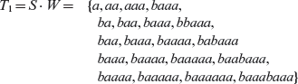
Let us now carefully examine how the test sequences generated by the W-method detect operation and transfer errors. Recall that the test set generated in the W-method is the set Ρ · W, given that the number of states in the IUT is the same as that in the specification. Thus, each test case t is of the form r · s where r belongs to the transition cover set Ρ and s to the characterization set W. We consider the application of t to the IUT as a two-phase process. In the first phase, input r moves the IUT from its initial state q₀ to some state q_i. In the second phase, the remaining input s moves the IUT to its final state q_j or q_j′. These two phases are shown in Figure 5.17.

Figure 5.17 Detecting errors using tests generated by the W-method. 

When the IUT is started in its initial state, say q₀, and excited with test t, it consumes the string r and arrives at some state q_i as shown in Figure 5.17. The output generated so far by the IUT is u where u = O(q₀, r). Continuing further in state q_i, the IUT consumes symbols in string s and arrives at state q_j. The output generated by the IUT while moving from state q_i to q_j is ν where v = O(q_i, s). If there is any operation error along the transitions traversed between states q₀ and q_i, then the output string u would be different from the output generated by the specification machine Μ when excited with r in its initial state. If there is any operation error along the transitions while moving from q_i to q_j, then the output wv would be different from that generated by M.

The detection of a transfer error is more involved. Suppose there is a transfer error in state q_i and s = as′. Thus, instead of moving to state q_k, where q_k = δ(q_i, a), the IUT moves to state q_k′ where q_k′ = δ(q_i, a). Eventually, the IUT ends up in state q_j′ where q_j′ = δ(q_k′ , s′). Note that this step may take several transitions and hence is indicated by a dotted arrow in the figure. Our assumption is that s is a distinguishing sequence in W for states q_i and q_j′ . In this case, w_v′ ≠ w_v. If s is not a distinguishing sequence for q_i and q_j′ then there must exist some other input as″ in W such that wv″ ≠ wv where v″ = O(q_k′ , s″).

5.7  The Partial W-method

The partial W-method, also known as the Wp-method, is similar to the W-method in that tests are generated from a minimal, complete, and connected FSM. However, the size of the test set generated using the Wp-method is often smaller than that generated using the W-method. This reduction is achieved by dividing the test generation process into two phases and making use of the state identification sets W_i, instead of the characterization set W, in the second phase. Furthermore, the fault detection effectiveness of the Wp-method remains the same as that of the W-method. The two-phases used in the Wp-method are described later in Section 5.7.1.

 

First, we define a state cover set S of an FSM Μ = (X, Y, Q, q₀, δ, O). S is a finite non-empty set of sequences where each sequence belongs to X* and for each state q_t ϵ Q, there exists an r ϵ S such that δ(q₀, r) = q_t. It is easy to see that the state cover set is a subset of the transition cover set and is not unique. Note that the empty string ϵ belongs to S which covers the initial state because, as per the definition of state transitions, δ(q₀, ϵ) = q₀.

 

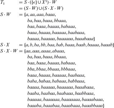
Example 5.15   In Example 5.11 the following transition cover set was constructed for machine Μ of Figure 5.13.

P = {ϵ, a, b, bb, ba, bob, baa, baab, baaa, baaab, baaaa}

The following subset of Ρ forms a state cover set for M.

S = {ϵ, b, ba, baa, baaa}

We are now ready to show how tests are generated using the Wp-method. As before, let M denote the FSM representation of the specification against which we are to test an IUT. Suppose that M contains n > 0 states and the IUT contains m > 0 states. The test set T derived using the Wp-method is composed of subsets T₁ and T₂, i.e. T = T₁ ∪ T₂. Computation of subsets T₁ and T₂ is shown below assuming that M and the IUT have an equal number of states, i.e. m = n.

 

Procedure for test generation using the Wp-method.

 

Step 1	Compute the transition cover set P, the state cover set S, the characterization set W, and the state identification sets Wi for M. Recall that S can be derived from P and the state identification sets can be computed as explained in Example 5.10.
Step 2	T1 = S ·W.
Step 3	Let W be the set of all state identification sets of M, i.e. W = {W1, W2, . . . , Wn}.
Step 4	Let R = {ri1 , ri2 , . . . rik} denote the set of all sequences that are in the transition cover set P but not in the state cover set S, i.e. R = P − S. Furthermore, let rij ϵ R be such that δ(q0, rij ) = qij.
Step 5	, where Wij ϵ W is the state identification set for state qij.

 

End of Procedure for test generation using the Wp-method.

The ⊗ operator used in the derivation of T₂ is known as the partial string concatenation operator. Having constructed the test set T, which consists of subsets Τ₁ and T₂, one proceeds to test the IUT as described in the next section.

 

5.7.1  Testing using the Wp-method for m = n

Given a specification machine M and its implementation under test, the Wp-method consists of a two-phase test procedure. In the first phase, the IUT is tested using the elements of T₁. In the second phase, the IUT is tested against the elements of T₂. Details of the two phases follow.

Phase 1: Testing the IUT against each element of T₁ tests each state for equivalence with the corresponding state in M. Note that a test sequence t in T₁ is of the kind uv where u ϵ S and v ϵ W. Suppose that δ(q₀, u) = q_i for some state q_i in M. Thus, the application of t first moves M to some state q_i. Continuing with the application of t to M, now in state q_i, generates an output different from that generated if v were applied to M in some other state q_j , i.e. O(q_i, v) ≠ O(q_j, v), for i ≠ j. If the IUT behaves as M against each element of T₁, then the two are equivalent with respect to S ·W. If not, then there is an error in the IUT.

Phase 2: While testing the IUT using elements of T₁ checks all states in the implementation against those in M, it may miss checking all transitions in the IUT. This is because T₁ is derived using the state cover set S and not the transition cover set P. Elements of T₂ complete the checking of the remaining transitions in the IUT against M.

To understand how, we note that each element t of T₂ is of the kind uv where u is in P but not in S. Thus, the application of t to M moves it to some state q_i where δ(q₀, u) = q_i. However, the sequence of transitions that M goes through is different from the sequence it goes through while being tested against elements of T₁ because u ∉ S. Next, M which is now in state q_i, is excited with v. Now v belongs to W_i which is the state identification set of q_i and hence this portion of the test will distinguish q_i from all other states with respect to transitions not traversed while testing against T₁. Thus, any transfer or operation errors in the transitions not tested using T₁ will be discovered using T₂.

 

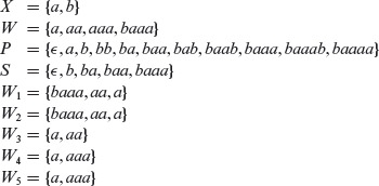
Example 5.16   Let us reconsider the machine in Figure 5.13 to be the specification machine M. First, various sets needed to generate the test set Τ are reproduced below for convenience.

Next, we compute set T₁ using Step 2.

Next, in accordance with Step 4 we obtain R as

R = P – S = {a , bb, bob, baab, baaab, baaaa}.

With reference to Step 4 and Figure 5.13, we obtain the following state transitions for the elements in R:

From the transitions given above, we note that when Μ is excited by elements a, bb, bab, baab, baaab, and baaaa, starting on each occasion in state q₁, it moves to states, q₁, q₄, q₁, q₅, q₅, and q₁, respectively. Thus, while computing T₂, we need to consider the state identification sets W₁, W₄, and W₅. Using the formula in Step 5, we obtain T₂ as follows.

The desired test set Τ = T₁ ∪ T₂. Note that Τ contains a total of 21 tests. This is in contrast to the 29 tests generated using the W-method in Example 5.12 when m = n.

The next example illustrates the Wp-method.

 

Example 5.17   Let us assume we are given the specification Μ as shown in Figure 5.15(a) and are required to test IUTs that correspond to designs M₁ and M₂ in Figure 5.15(b) and (c), respectively. For each test, we proceed in two phases as required by the Wp-method.

 

Testing using the Wp-method proceeds in two phases. In the first phase, elements of test T₁ are applied followed by those of test T₂ where T₁ and T₂ are subsets of the tests generated using the Wp-method. Tests in Τ₁ ensure that each state is reached and distinguished from the rest. However, doing so might miss the testing of all transitions which is done in phase 2 using tests from T₂.

Test M₁, phase 1: We apply each element t of T₁ to the IUT corresponding to M₁ and compare M₁(t) with the expected response M(t). To keep this example short, let us consider test t = baaaaaa. We obtain M₁(t) = 1101001. On the contrary, the expected response is M(t) = 1101000. Thus, test input t has revealed the transfer error in state q₂.

Test M₁, phase 2: This phase is not needed to test M₁. In practice, however, one would test M₁ against all elements of T₂. You may verify that none of the elements of T₂ reveal the transfer error in M₁.

Test M₂, phase 1: Test t = baabaaa that belongs to T₁ reveals the error as M₂(t) = 1100100 and Μ(t) = 1101000.

Test M₂, phase 2: Once again this phase is not needed to reveal the error in M₂.

Note that in both the cases in the example above, we do not need to apply phase 2 of the Wp-method to reveal the error. For an example that does require phase 2 to reveal an implementation error, refer to Exercise 5.15 that shows an FSM and its erroneous implementation and requires the application of phase 2 for the error to be revealed. However, in practice, one would not know whether or not phase 1 is sufficient. This would lead to the application of both phases and hence all tests. Note that tests in phase 2 ensure the coverage of all transitions. While tests in phase 1 might cover all transitions, they might not apply the state identification inputs. Hence, all errors corresponding to the fault model in Section 5.4 are not guaranteed to be revealed by tests in phase 1.

5.7.2  Testing using the Wp-method for m > n

The procedure for constructing tests using the Wp-method can be modified easily when the number of states in the IUT is estimated to be larger than that in the specification, i.e. when m > n. Steps 2 and 5 of the procedure described earlier need to be modified.

 

For m = n, we compute T₁ = S · W. For m > n we modify this formula so that T₁ = S · Ζ where Ζ = X[m – n] · W as explained in Section 5.6.4. Recall that T₁ is used in phase 1 of the test procedure. T₁ is different from Τ derived from the W-method in that it uses the state cover set S and not the transition cover set P. Hence, T₁ contains fewer tests than Τ except when P = S.

To compute T₂, we first compute R as in Step 4. Recall that R contains only those elements of the transition cover set Ρ that are not in the state cover set S. Let R = Ρ – S = {r_i1, r_i2, . . . r_ik}. As before, r_ij ϵ R moves Μ from its initial state to state q_ij, i.e. δ(q₀, r_ij) = q_ij. Given R, we derive T₂ as follows.

where δ(q₀, r_ij) = q_ij δ(q_ij, u) = q_l, and W_l ϵ W is the identification set for state q_l.

The basic idea underlying phase 2 is explained in the following. The IUT under test is exercised so that it reaches some state q_i from the initial state q₀. Let u denote the sequence of input symbols that move the IUT from state q₀ to q_i. As the IUT contains m > n states, it is now forced to take an additional (m – n) transitions. Of course, it requires (m – n) input symbols to force the IUT for that many transitions. Let ν denote the sequence of symbols that move the IUT from state q_i to state q_j in (m – n) steps. Finally, the IUT receives an input sequence of symbols, say w, that belong to the state identification set W_j. Thus, one test for the IUT in phase 2 is comprised of the input sequence uvw.

Notice that the expression to compute T₂ consists of two parts. The first part is R and the second part is the partial string concatenation of X[m – n] and W. Thus, a test in T₂ can be written as uvw where u ϵ R is the string that takes the IUT from its initial state to some state q_i string ν ϵ X[m – n] takes the IUT further to state q_j and string w ϵ W_j takes it to some state q_l. If there is no error in the IUT, then the output string generated by the IUT upon receiving the input uvw must be the same as the one generated when the design specification Μ is exercised by the same string.

 

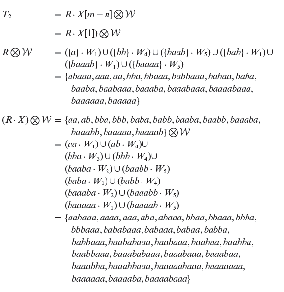
Example 5.18   Let us construct a test set using the Wp-method for machine Μ in Figure 5.13 given that the corresponding IUT contains an extra state. For this scenario, we have n = 5 and m = 6. Various sets needed to derive Τ are reproduced here for convenience.

First, Τ₁ is derived as S · X[1] · W. Recall that X[1] denotes the set {ϵ}∪ X¹.

T₁ contains a total of 60 tests of which 20 are in S · W and 40 in S · X · W. To obtain T₂, we note that R = Ρ – S = {a, bb, bab, baab, baaab, baaaa}. T₂ can now be computed as follows.

T₂ contains a total of 38 tests. In all the entire test set Τ = T₁ ∪ T₂ contains 81 tests. This is in contrast to a total of 44 tests that would be generated by the W-method. (See Exercises 5.16 and 5.17.)

5.8  The UIO-Sequence Method

The W-method uses the characterization set W of distinguishing sequences as the basis to generate a test set for an IUT. The tests so generated are effective in revealing operation and transfer faults. However, the number of tests generated using the W-method is usually large. Several alternative methods have been proposed that generate fewer test cases. In addition, these methods are either as effective or nearly as effective as the W-method in their fault detection capability. We now introduce two such methods. A method for test generation based on unique input/output sequences is presented in this section.

5.8.1  Assumptions

The UIO method generates tests from an FSM representation of the design. All the assumptions stated in Section 5.6.1 apply to the FSM that is input to the UIO test generation procedure. In addition, it is assumed that the IUT has the same number of states as the FSM that specifies the corresponding design. Thus, any errors in the IUT are transfer and operations errors only as shown in Figure 5.12.

5.8.2  UIO sequences

A unique input/output sequence, abbreviated as UIO sequence, is a sequence of input and output pairs that distinguishes a state of an FSM from the remaining states. Consider FSM Μ = (Χ, Y, Q, q₀, δ, O). A UIO sequence of length k for some state s ϵ Q is denoted as UIO(s) and looks like the following sequence

 

UIO(s) = i₁/o₁ · i₂/o₂ · . . . i_(k−1)/o_(k−1) · i_k/o_k.

In the sequence given above, each pair a/b consists of an input symbol a that belongs to the input alphabet X and an output symbol b that belongs to the output alphabet Y. As before, the dot symbol (·) denotes string concatenation. We refer to the input portion of a UIO(s) as in(UIO(s)) and to its output portion as out(UIO(s)). Using this notation for the input and output portions of UIO(s), we can rewrite UIO(s) as

in(UIO(s)) = i₁ · i₂ · . . . i_(k–1) · i_k, and out(UIO(s)) = ο₁ · ο₂·… o_(k–1) · o_k.

When the sequence of input symbols that belong to in(UIO(s)) is applied to Μ in state s, the machine moves to some state t and generates the output sequence out(UIO(s)). This can be stated more precisely as follows,

δ(s, in(UIO(s)) = t, O(s, in(UIO(s))) = out(UIO(s)).

 

A formal definition of unique input/output sequences follows. Given an FSM Μ = (X, Y, Q, q₀, δ, O), the unique input/output sequence for state s ∈ Q, denoted as UIO(s), is a sequence of one or more edge labels such that the following condition holds.

O(s, in(UIO(s))) ≠ O(t, in(UIO(s))), for all t ∈ Q, t ≠ s.

The next example offers UIO sequences for a few FSMs. The example also shows that there may not exist any UIO sequence for one or more states in an FSM.

 

Example 5.19   Consider machine M₁ shown in Figure 5.18. The UIO sequence for each of the six states in M₁ is given below.

Using the definition of UIO sequences, it is easy to check whether or not a UIO(s) for some state s is indeed a unique input/output sequence. However, before we perform such a check, we assume that the machine generates an empty string as the output if there does not exist an outgoing edge from a state on some input. For example, in Machine M₁ there is no outgoing edge from state q₁ for input c. Thus, M₁ generates an empty string when it encounters a c in state q₁. This behavior is explained in Section 5.8.3.

Figure 5.18 Two FSMs used in Example 5.19. There is a UIO sequence for each state in Machine M₁. There is no UIO sequence for state q₁ in Machine M₂.

State (s)	UIO (s)
q1	a/0 · c/1
q2	c/1· c/1
q3	b/1· b/1
q4	b/1· c/0
q5	c/0
q6	c/1· a/0

Let us now perform two sample checks. From the table above we have UIO(q₁) = a/0 · c/1. Thus, in(UIO(q₁) = ac, out(UIO(q₁)) = 01. Applying the sequence a · c to state q₂ produces the output sequence 0 which is different from 0₁ generated when a · c is applied to M1 in state q₁. Similarly, applying ac to Machine M₁ in state q₅ generates the output pattern 0 which is, as before, different from that generated by q₁. You may now perform all other checks to ensure that indeed the UIOs given above are correct.

 

Example 5.20   Now consider Machine M₂ in Figure 5.18. The UIO sequences for all states, except state q₁, are listed below. Notice that there does not exist any UIO sequence for state q₁.

State (s)	UIO (s)
q1	None
q2	a/1
q3	b/1

5.8.3  Core and non-core behavior

An FSM must satisfy certain constraints before it is used for constructing UIO sequences. First there is the “connected assumption” which implies that every state in the FSM is reachable from its initial state. The second assumption is that the machine can be applied a reset input in any state that brings it to its start state. As has been explained earlier, a null output is generated upon the application of a reset input.

 

The third assumption is known as the completeness assumption. According to this assumption, an FSM remains in its current state upon the receipt of any input for which the state transition function δ is not specified. Such an input is known as a non-core input. In this situation, the machine generates a null output. The completeness assumption implies that each state contains a self-loop that generates a null output upon the receipt of an unspecified input. The fourth assumption is that the FSM must be minimal. A machine that depicts only the core behavior of an FSM is referred to as its core-FSM. The following example illustrates the core behavior.

 

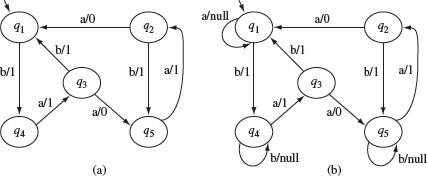
Example 5.21   Consider the FSM in Figure 5.19(a) that is similar to the one in Figure 5.13. Note that states q₁, q₄, and q₅ have no transitions corresponding to inputs a, b, and b, respectively. Thus, this machine does not satisfy the completeness assumption.

As shown in Figure 5.19(b), additional edges are added to this machine in states q₁, q₄, and q₅. These edges represent transitions that generate null output. Such transitions are also known as erroneous transitions. Figure 5.19(a) shows the core behavior corresponding to the machine in Figure 5.19(b).

While determining the UIO sequences for a machine, only the core behavior is considered. The UIO sequences for all states of the machine shown in Figure 5.19(a) are given below.

State (s)	UIO (s)
q1	b/1· a/1/· b/1· b/1
q2	a/0· b/1
q3	b/1· b/1
q4	a/1· b/1· b/1
q5	a/1· a/0· b/1

Note that the core behavior exhibited in Figure 5.19 is different from that in the original design in Figure 5.13. Self-loops that generate a null output, are generally not shown in a state diagram that depicts the core behavior. The impact of removing self-loops, that generate a non-null output, on the fault detection capability of the UIO method will be discussed in Section 5.8.9. In Figure 5.19, the set of core edges is {(q₁, q₄), (q₂, q₁), (q₂, q₅), (q₃, q₁), (q₃, q₅), (q₄, q₃), (q₅, q₂), (q₁, q₁), (q₂, q₂), (q₃, q₃), (q₄, q₄), (q₅, q₅)}.

Figure 5.19 (a) An incomplete FSM. (b) Addition of null transitions to satisfy the completeness assumption. 

The core-behavior of an FSM does not include self loops that generate null outputs.

During a test, one wishes to determine if the IUT behaves in accordance with its specification. An IUT is said to conform strongly to its specification if it generates the same output as its specification for all inputs. An IUT is said to conform weakly to its specification if it generates the same output as that generated by the corresponding core-FSM.

 

Example 5.22   Consider an IUT that is to be tested against its specification Μ as in Figure 5.13. Suppose that the IUT is started in state q₁ and the one symbol sequence a is input to it and the IUT outputs a null sequence, i.e. the IUT does not generate any output. In this case, the IUT does not conform strongly to M. However, on input a, this is exactly the behavior of the core-FSM. Thus, if the IUT behaves exactly as the core-FSM shown in Figure 5.19(a), then it conforms weakly to M.

5.8.4  Generation of UIO sequences

The UIO sequences are essential to the UIO-sequence method for generating tests from a given FSM. In this section, we present an algorithm for generating the UIO sequences. As mentioned earlier, a UIO sequence might not exist for one or more states in an FSM. In such a situation, a signature is used instead. An algorithm for generating UIO sequences for all states of a given FSM follows.

 

Procedure for generating UIO sequences

 

Input:	(a) An FSM M = (X, Y, Q, q0, δ, O) where |Q| = n. (b) State s ∈ Q.
Output:	UIO(s) contains a unique input/output sequence for state s; UIO(s) is empty if no such sequence exists.
Procedure:	gen-UIO(S)
/*	Set(l) denotes the set of all edges with label l.
	label(e) denotes the label of edge e.
	A label is of the kind a/b where a ∈ X and b ∈ Y.
	head(e) and tail(e) denote, respectively, the head and tail states of edge e. */

 

Step 1	For each distinct edge label el in the FSM, compute Set(el).
Step 2	Compute the set Oedges(s) of all outgoing edges for state s. Let NE = |Oedges|.
Step 3	For 1 ≤ i ≤ NE and each edge ei ∈ Oedges, compute Oled[i], Opattern[i], and Oend[i] as follows:
3.1	Oled[i] = Set(label(ei)) − {ei}.
3.2	Opattern[i] = label(ei).
3.3	Oend[i] = tail(ei).
Step 4	Apply algorithm gen-1-uio(s) to determine if UIO(s) consists of only one label.
Step 5	If simple UIO sequence found then return UIO(s) and terminate this algorithm, otherwise proceed to the next step.
Step 6	Apply the gen-long-uio(s) procedure to generate longer UIO(s).
Step 7	If longer UIO sequence found then return UIO(s) and terminate this algorithm, else return with an empty UIO(s)

 

End of procedure gen-uio.

 

Procedure gen-1-uio

Input:	State s ∈ Q.
Output:	UIO(s) of length 1 if it exists, an empty string otherwise.
Procedure:	gen-1-UIO (State S):

 

Step 1

If Oled[i] = Ø for 1 ≤ i ≤ NE then return UIO(s) = label(ei) otherwise return UIO(s) = "".

 

End of procedure gen-1-uio

 

Procedure for generating longer UIO sequences

Input:	(a) Oedges, Opattern, Oend, and Oled as computed in gen-uio.
	(b) State s ∈ Q.
Output:	UIO(s) contains a unique input/output sequence for state s and is empty if no such sequence exists.
Procedure:	gen-long-uio (State s)

 

Step 1	Let L denote the length of the UIO sequence being examined. Set L = 1. Let Oedges denote the set of outgoing edges from some state under consideration.
Step 2	Repeat steps below while L < 2n2 or the procedure is terminated prematurely.
2.1	Set L = L + 1 and k = 0. Counter k denotes the number of distinct patterns examined as candidates for UIO(s). The following steps attempt to find a UIO(s) of size L.
2.2	Repeat steps below for i = 1 to NE. Index i is used to select an element of Oend to be examined next. Note that Oend[i] is the tail state of the pattern in Opattern[i].
2.2.1	Let Tedges(t) denote the set of incoming edges to state t. Compute Tedges(Oend[i]).
2.2.2	For each edge te ∈ Tedges execute gen-L-UIO(te) until either all edges in Tedges have been considered or a UIO(s) is found.
2.3	Prepare for the next iteration. Set k = NE. For 1 ≤ j ≤ k, set Opattern[j] = Pattern[j], Oend[j] = End[j], and Oled[j] = Led[j]. If the loop termination condition is not satisfied, then go back to Step 2.1 and search for UIO of the next higher length, else return to gen-uio indicating a failure to find any UIO for state s.

 

End of procedure gen-long-uio

 

Procedure for generating UIO sequences of length L>1.

Input:	Edge te from procedure gen-long-UIO .
Output:	UIO(s) contains a unique input/output sequence of length L for state s and is empty if no such sequence exists.
Procedure:	gen-L-uio ( edge te)

 

Step 1	k = k + 1, Pattern[k] = Opattarn[k] · label(te). This could be a possible UIO.
Step 2	End[k] = tail(te) and Led[k] = Ø.
Step 3	For each pair oe ∈ Oled[i], where h = head(oe) and t = tail(oe), repeat the next step.
3.1	Execute the next step for each edge o ∈ Oedges(t).
3.1.1	If label(o) = label(te) then Led[k] = Led[k]∪{(head(oe), tail(o))}.
Step 4	If Led[k] = Ø, then UIO of length L has been found. Set UIO(s) = Pattern[k] and terminate this and all procedures up until the main procedure for finding UIO for a state. If Led[k] ≠ Ø, then no UIO of length L has been found corresponding to edge te. Return to the caller to make further attempts.

 

End of Procedure gen-L-uio

5.8.5  Explanation of gen-uio

The idea underlying the generation of a UIO sequence for state s can be explained as follows. Let M be the FSM under consideration and s a state in M for which a UIO is to be found. Let E(s) = e₁e₂ . . . e_k be a sequence of edges in M such that s = head(e₁), tail(e_i) = head(e_i+1), and 1 ≤ i < k.

 

For E(s), we define a string of edge labels as label(E(s)) = l₁ · l₂ · . . . l_k−1 · l_k, where l_i = label(e_i), 1 ≤ i ≤ k, is the label of edge e_i. For a given integer l > 0, we find if there is a sequence E(s) of edges starting from s such that label(E(s)) ≠ label(E(t)), s ≠ t for all states t in M. If there is such an E(s), then label(E(s)) is a UIO for state s. The uniqueness check is performed on E(s) starting with l = 1 and continuing for l = 2, 3, ... until a UIO is found or l = 2n², where n is the number of states in M. Note that there can be multiple UIOs for a given state though the algorithm generates only one UIO, if it exists.

The gen-uio algorithm is explained with reference to Figure 5.20. Algorithm gen-uio for state s begins with the computation of some sets used in the subsequent steps. First, the algorithm computes Set(el) for all distinct labels el in the FSM. Set(el) is the set of all edges that have el as their label.

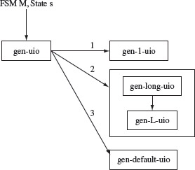
Figure 5.20 Flow of control across various procedures in gen-uio.

Next, the algorithm computes the set Oedges(s) which is the set of outgoing edges from state s. For each edge e in Oedges(s), the set Oled[e] is computed. Oled[e] contains all edges in Set(label(e)) except for the edge e. The tail state of reach edge in Oedges is saved in Oend[e]. The use of Oled will become clear later in Example 5.27.

 

Example 5.23   To find UIO(q₁) for machine M₁ in Figure 5.18, Set, Oedges and Oled are computed as follows.

Distinct labels in M₁ = {a/0, b/1, c/0, c/1}

Set(a/0) = {(1, 2), (2, 3), (3, 4)_a/0}

Set(b/1) = {(3, 4), (4, 5)}

Set(c/0) = {(5, 6)}

Set(c/1) = {(2, 6), (6, 1)}

Oedges(q) = {(1, 2)}, NE = 1

Oled[1] = {(2, 3), (3, 4)_a/0}

Oend[1] = q₂

Opattern[1] = a/0

Next, gen-1-uio is called in an attempt to generate a UIO of length 1. For each edge e_i ∈ Oedges, gen-1-uio initializes Opattern[i] to label(e_i) and Oend[i] to tail(e_i). Opattern and Oend are used subsequently by gen-uio in case a UIO of length 1 is not found. gen-1-uio now checks if the label of any of the outgoing edges from s is unique. This is done by checking if Oled[i] is empty for any e_i ∈ Oedges(s). Upon return from gen-1-uio, gen-uio terminates if a UIO of length 1 was found, otherwise it invokes gen-long-uio in an attempt to find a UIO of length greater than 1. gen-longer-uio attempts to find UIO of length L > 1 until it finds one, or L = 2n².

 

Example 5.24   As an example of a UIO of length 1, consider state q₅ in Machine M₁ in Figure 5.18. The set of outgoing edges for state q₅ is {(5, 6)}. The label of {(5, 6)} is c/0. Thus, from gen-uio and gen-1-uio, we get Oedges(q₅) = {(5, 6)}, Oled[1] = Ø, Oen[1] = q₆, and Opattern[1] = label(e₁) = c/0. As Oled[1] = Ø, state q₅ has a UIO of length 1 which is Opattern[1], i.e. c/0.

 

Example 5.25   As an example of a state for which a UIO of length 1 does not exist, consider state q₃ in Machine M₁ shown in Figure 5.18. For this state, we get the following sets:

Oedges(q₃) = {(3, 4)_a/0, (3, 4)_b/1}, NE = 2

Oled[1] = {(1, 2), (2, 3)}, Oled[2] = {(4, 5)} 

Opattern[1] = a/0, Opattern[2] = b/1

Oend[1] = q₄, Oend[2] = q₄

Opattern[1] = a/0, Opattern[2] = b/1

As no element of Oled is empty, gen-1-uio concludes that state q₃ has no UIO of length 1 and returns to gen-uio.

In the event gen-1-uio fails, procedure gen-long-uio is invoked. The task of gen-long-uio is to check if a UIO(s) of length two or more exists. To do so, it collaborates with its descendent gen-L-uio. An incremental approach is used where UIOs of increasing length, starting at two, are examined until either a UIO is found or one is unlikely to be found, i.e. a maximum length pattern has been examined.

To check if there is UIO of length L, gen-long-uio computes the set Tedges(t) for each edge e ∈ Oedges(s), where t = tail(e). For L = 2, Tedges(t) will be a set of edges outgoing from the tail state t of one of the edges of state s. However, in general, Tedges(t) will be the set of edges going out of a tail state of some edge outgoing from state s′, where s′ is a successor of s. After initializing Tedges, gen-L-uio is invoked iteratively for each element of Tedges(t). The task of gen-L-uio is to find whether or not there exists a UIO of length L.

 

Example 5.26   There is no UIO(q₁) of length one. Hence gen-long-uio is invoked. It begins by attempting to find a UIO of length two, i.e. L = 2. From gen-uio, we have Oedges(q₁) = {(1, 2)}. For the lone edge in Oedges, we get t = tail((1, 2)) = q₂. Hence Tedges(q₂), which is the set of edges out of state q₂, is computed as follows:

Tedges(q₂) = {(2, 3), (2, 6)}

 

The gen-long-uio procedure is invoked when there is no UIO sequence of length 1.

gen-L-uio is now invoked first with edge (2, 3) as input to determine if there is a UIO of length two. If this attempt fails, then gen-L-uio is invoked with edge (2, 6) as input.

To determine if there exists a UIO of length L corresponding to an edge in Tedges, gen-L-uio initializes Pattern[k] by catenating the label of edge te to Opattern[k]. Recall that Opattern[k] is of length (L – 1) and has been rejected as a possible UIO(s). Pattern[k] is of length L and is a candidate for UIO(s). Next, the tail of te is saved in End[k]. Here, k serves as a running counter of the number of patterns of length L examined.

Next, for each element of Oled[i], gen-L-uio attempts to determine if indeed Pattern[k] is a UIO(s). To understand this procedure, suppose that oe is an edge in Oled[i]. Recall that edge oe has the same label as the edge e_i and that e_i is not in Oled[i]. Let t be the tail state of oe and Oedges(t) the set of all outgoing edges from state t. Then, Led[k] is the set of all pairs (head(oe), tail(oe)) such that label(te) = label(oe) for all ο ∈ Oedges(t).

Note that an element of Led[k] is not an edge in the FSM. If Led[k] is empty after having completed the nested loops in Step 3, then Pattern[k] is indeed a UIO(s). In this case, the gen-uio procedure is terminated and Pattern[te] is the desired UIO. If Led[k] is not empty, then gen-L-uio returns to the caller for further attempts at finding UIO(s).

 

Example 5.27   Continuing Example 5.26, suppose that gen-L-uio is invoked with i = 1 and te = (2, 3). The goal of gen-L-uio is to determine if there is a path of length L starting from state head(te) that has its label same as Opattern[i] · label(te).

Pattern[i] is set to a/0 · a/0 because Opattern[i] = a/0 and label((2, 3)) = a/0. End[i] is set to tail(2, 3) which is q₃. The outer loop in Step 3 examines each element oe of Oled[1]. Let oe = (2, 3) for which we get h = q₂ and t = q₃. The set Oedges(q₃) = {(3, 4)_a/0, (3, 4)_b/1)}. Step 3.1 now iterates over the two elements of OutEedges(q₃) and updates Led[i]. At the end of this loop, we have Led[i] = {(2, 4)} because label((3, 4)_a/0) = label((2, 3)).

Continuing with the iteration over Oled[1], oe is set to (3, 4)_a/0 for which h = q₂ and t = q₄. The set Oedges(q₄) = {(4, 5)}. Iterating over Oedges(q₄) does not alter Led[i] because label((4, 5)) ≠ label((3, 4)_a/0).

The outer loop in Step 3 is now terminated. In the next step, i.e. Step 4, Pattern[i] is rejected and gen-L-uio returns to gen-long-uio.

Upon return from gen-L-uio, gen-long-uio once again invokes it with i = 1 and te = (2, 6). Led[2] is determined during this call. To do so, Pattern[2] is initialized to a/0 · c/1 because Opattern[i] = a/0 and label(2, 6) = c/1, and End[2] to q₆.

Once again, the procedure iterates over elements oe of Oled. For oe = (2, 3), we have as before, Oedges(q₃) = {(3, 4)_a/0, (3, 4)_b/1}. Step 3.1 now iterates over the two elements of Oedges(q₃). In Step 1, none of the checks is successful as label((2, 6)) is not equal to label((3, 4)_a/0) or to label((4, 5)). The outer loop in Step 3 is now terminated. In the next step, i.e. Step 4, Pattern[2] is accepted as UIO(q₁).

It important to note that Led[i] does not contain edges. Instead, it contains one or more pairs of states, (s₁, s₂) such that a path in the FSM from state s₁ to state s₂ has the same label as Pattern[i]. Thus, at the end of the loop in Step 3 of gen-L-uio, an empty Led[i] implies that there is no path of length L from head(te) to tail(te) with a label same as Pattern[i].

A call to gen-long-uio either terminates the gen-uio algorithm abruptly indicating that UIO(s) has been found, or returns normally indicating that UIO(s) is not found, and any remaining iterations should now be carried out. Upon a normal return from gen-L-uio, the execution of gen-long-uio resumes at Step 2.3. In this step, the existing Pattern, Led, and End data is transferred to Opattern, Oled, and Οend, respectively. This is done in preparation for the next iteration to determine if there exists a UIO of length (L + 1). In case a higher length sequence remains to be examined, the execution resumes from Step 2.2, else the gen-long-uio terminates without having determined a UIO(s).

 

Example 5.28   Consider M₂ in Figure 5.18. We invoke gen-uio(q₁) to find a UIO for state q₁. As required in Steps 1 and 2, we compute Set for each distinct label and the set of outgoing edges Oedges(q₁).

 

Distinct labels in M₂ = {a/0, a/1, b/0, b/1}

Set(a/0) = {(1, 2), (3, 2)}

Set(a/1) = {(2, 1)}

Set(b/0) = {(1, 3), (2, 3)}

Set(b/1) = {(3, 1)}

Oedges(q₁) = {(1, 2), (1, 3)}

NE = 2

Next, as directed in Step 3, we compute Oled and Οend for each edge in Oedges(q₁). The edges in Oedges are numbered sequentially so that edge (1, 2) is numbered 1 and edge (1, 3) is numbered 2.

Oled[1] = {(3, 2)}

Oled[2] = {(2, 3)}

Oend[1] = q₂

Oend[2] = q₃

Opattern[1] = a/0

Opattern[2] = b/0

gen-1-uio(q₁) is now invoked. As Oled[1] and Oled[2] are nonempty, gen-1-uio fails to find a UIO of length one and returns. We now move to Step 6 where procedure gen-long-uio is invoked. It begins by attempting to check if a UIO of length two exists. Towards this goal, the set Tedges is computed for each edge in Oedges at Step 2.2.1 of gen-long-uio. First, for i = 1, we have Oled[1] = (3, 2) whose tail is state q₂. Thus, we obtain Tedges(q₂) = {((2, 3), (2, 1)}.

The loop for iterating over the elements of Tedges begins at Step 2.2.2. Let te = (2, 3). gen-L-uio is invoked with te as input and the value of index i as 1. Inside gen-L-uio, k is incremented to 1 indicating that the first pattern of length two is to be examined. Pattern[1] is set to a/0 · b/0, End[1] to 3, and Led[1] initialized to the empty set.

The loop for iterating over the two elements of Oled begins at Step 3. Let oe = (3, 2) for which h = 3, t = 2, and Oedges(2) = {(2, 1), (2, 3)}. We now iterate over the elements of Oedges as indicated in Step 3.1. Let ο = (2, 1). As labels of (2, 1) and (2, 3) do not match, Led[1] remains unchanged. Next, ο = (2, 3). This time we compare labels of ο and te, which are the same edges. Hence, the two labels are the same. As directed in Step 3.1.1, we set Led[1] = (head(oe), tail(o)) = (3, 3). This terminates the iteration over Oedges. This also terminates the iteration over Oled as it contains only one element.

In Step 4, we find that Led[1] is not empty and therefore reject Pattern[1] as a UIO for state q₁. Notice that Led[1] contains a pair (3, 3) which implies that there is a path from state q₃ to q₃ with the label identical to that in Pattern[1]. A quick look at the state diagram of M₂ in Figure 5.18 reveals that indeed the path q₃ → q₂ → q₃ has the label a/0 · b/0 which is the same as in Pattern[1].

Control now returns to Step 2.2.2 in gen-long-uio. The next iteration over Tedges(q₂) is initiated with te = (2, 1). gen-L-uio is invoked once again but this time with index i = 1 and te = (2, 1). The next pattern of length two to be examined is Pattern[2] = a/0 · a/1. We now have End[2] = 1 and Led[2] = Ø. Iteration over elements of Oled[1] begins. Once again let oe = (3, 2) for which h = 3, t = 2, and Oedges(2) = {(2, 1), (2, 3)}. Iterating over the two elements of Oeges we find that the label of te matches that of edge (2, 1) and not of edge (2, 3). Hence, we get Led[2] = (head(oe), tail(2, 1)) = (3, 1) implying that Pattern[2] is the same as the label of the path from state q₃ to state q₁. The loop over Oled also terminates and control returns to gen-long-uio.

In gen-long-uio, the iteration over Tedges now terminates as we have examined both edges in Tedges. This also completes the iteration for i = 1 which corresponds to the first outgoing edge of state q₁. We now repeat Step 2.2.2 for i = 2. In this iteration, the second outgoing edge of state q₁, i.e. edge (1, 3), is considered. Without going into the fine details of each step, we leave it to you to verify that at the end of the iteration for i = 2, we get the following.

Pattern[3] = b/0 · a/0

Pattern[4] = b/0 · b/1

End[3] = 2

End[4] = 1

Led[3] = (2, 2)

Led[4] = (2, 1)

This completes the iteration set up in Step 2.2. We now move to Step 3. This step leads to the following values of Opattern, Oled, and Oend.

Opattern[1] = Pattern[1] = a/0 · b/0

Opattern[2] = Pattern[2] = a/0 · a/1

Opattern[3] = Pattern[3] = b/0 · a/0

Opattern[4] = Pattern[4] = b/0 · b/1

 

Oend[1] = End[1] = 3

Oend[2] = End[2] = 1

Oend[3] = End[3] = 2

Oend[4] = End[4] = 1

 

Oled[1] = Led[1] = (3, 3)

Oled[2] = Led[2] = (3, 1)

Oled[3] = Led[3] = (2, 2)

OIed[4] = Led[4] = (2, 1)

 

The while-loop continues with the new values of Opattern, Οend, and Oled. During this iteration L = 3 and hence patterns of length three will be examined as candidates for UIO(q₁). The patterns to be examined next will have at least one pattern in Opattern as its prefix. For example, one of the patterns examined for i = 1 is a/0 · b/0 · a/0.

The gen-L-uio procedure is invoked first with e = (1, 2) and te = (2, 3) in Step 2.2.2. It begins with Pattern[1] = a/0 · b/0 and End[1] = 3.

 

Example 5.29   This example illustrates the workings of procedure gen-uio(s) by tracing through the algorithm for Machine M₁ in Figure 5.18. The complete set of UIO sequences for this machine is given in Example 5.19. In this example, we sequence through gen-uio(s) for s = q₁. The trace follows.

gen-uio	Input : State q1
Step 1	Find the set of edges for each distinct label in M1. There are four distinct labels in M1, namely a/0, b/1, c/0, and c/1. The set of edges for each of these four labels is given below.
	Set(a/0) = {(1, 2), (2, 3), (3, 4)}
	Set(b/1) = {(3, 4), (4, 5)}
	Set(c/0) = {(5, 6)}
	Set(c/1) = {(2, 6), (6, 1)}
Step 2	It is easily seen from the state transition function of M1 that the set of outgoing edges from state q1 is {(1,2)}. Thus, we obtain Oedges(q1) = {(1, 2)} and NE = 1.
Step 3	For each edge in Oedges, we compute Oled, Opattern, and Oend.
	Oled[1] = {(1, 2), (2, 3), (3, 4)a/0} – {(1, 2)} = {(2, 3), (3, 4)a/0}.
	Opattern[1] = label((1, 2)) = a/0, and
	Oend[1] = tail((1, 2)) = 2.
Step 4	Procedure gen-1-UIO is invoked with state q1 as input. In this step, an attempt is made to determine if there exists a UIO sequence of length 1 for state q1.
gen-1-UIO	Input : State q1
Step 1	Now check if any element of Oled contains only one edge. From the computation done earlier, note that there is only one element in Oled, and that this element, Oled[1], contains two edges.
	Hence, there is no UIO(q1) with only a single label. The gen-1-UIO procedure is now terminated and the control returns to gen-UIO.
gen-uio	Input : State q1
Step 5	Determine if a simple UIO sequence was found. As it has not been found, move to the next step.
Step 6	Procedure gen-long-UIO is invoked in an attempt to generate a longer UIO(q1).
gen-long-UIO	Input : State q1
Step 1	L = 1.
Step 2	Start a loop to determine if a UIO(q1) of length greater than 1 exists. This loop terminates when a UIO is found or when L = 2n2, which for a machine with n = 6 states translates to L = 72. Currently, L is less than 72 and hence continue with the next step in this procedure.
Step 2.1	L = 2 and k = 0.
Step 2.2	Start another loop to iterate over the edges in Oedges. Set i = 1 and ei = (1, 2).
Step 2.2.1	t = tail((1, 2)) = 2. Tedges(2) = {(2, 3), (2, 6)}.
Step 2.2.2	Yet another loop begins at this point. Loop over the elements of Tedges. First set te = (2, 3) and invoke gen-L-UIO.
gen-L-UIO	Input : te = (2, 3)
Step 1	k = 1, Pattern[1] = Opattern[1] · label((2, 3)) = a/0 · a/0.
Step 2	End[1] = 3, Led[1] = Ø.
Step 3	Now iterate over elements of Oled[1] = {(2, 3), (3, 4)a/0}. First select oe = (2, 3) for which h = 2 and t = 3.
Step 3.1	Another loop is set up to iterate over elements of Oedges(q3) = {(3, 4)a/0, (3, 4)b/1}. Select o = (3, 4)a/0.
Step 3.1.1	As label((3, 4)a/0) = label((2, 3)), set Led[1] = {(2, 4)}.
	Next select o = (3, 4)b/1 and execute Step 3.1.1.
Step 3.1.1	As label((2, 3)) ≠ label((3, 4)b/1), no change is made to Led[1].
	The iteration over Oedges terminates.
	Next, continue from Step 3.1 with oe = (3, 4)a/0 for which h = 3 and t = 4.
Step 3.1	Another loop is set up to iterate over elements of Oedges(4) = {(4, 5)}, select o = (4, 5).
Step 3.1.1	As label((4, 5)) ≠ label((3, 4)a/0) no change is made to Led[1].
	The iterations over Oedges and Oled[1] terminate.
Step 4	Led[1] is not empty which implies that this attempt to find a UIO(q1) has failed. Note that in this attempt the algorithm checked if a/0 · a/0 is a valid UIO(q1). Now return to the caller.
gen-long-UIO	Input : State q1
Step 2.2.2	Select another element of Tedges and invoke gen-L-UIO (e, te). For this iteration te = (2, 6).
gen-L-UIO	Input : te = (2, 6)
Step 1	k = 2, Pattern[2] = Opattern[1] · label((2, 6)) = a/0 · c/1.
Step 2	End[2] = 6, Led[2] = Ø.
Step 3	Iterate over elements of Oled[1] = {(2, 3), (3, 4)a/0}. First select oe = (2, 3) for which h = 2 and t = 3.
Step 3.1	Another loop is set up to iterate over elements of Oedges(3) = {(3, 4)a/0, (3, 4)b/1}, select o = (3, 4)a/0.
Step 3.1.1	As label((3, 4)a/0) ≠ label((2, 6)), do not change Led[2].
	Next select o = (3, 4)b/1 and once again execute Step 3.1.1.
Step 3.1.1	As label((2, 6)) ≠ label((3, 4)b/1), do not change Led[2]. The iteration over Oedges terminates.
	Next continue from Step 3.1 with oe = (3, 4)a/0 for which h = 3 and t = 4.
Step 3.1	Another loop is set up to iterate over elements of Oedges(4) = {(4, 5)}, select o = (4, 5).
Step 3.1.1	As label((4, 5) ≠ label((2, 6)) no change is made to Led[2].
	The iterations over Oedges and Oled[2] terminate.
Step 4	Led[2] is empty. Hence UIO(q1) = Pattern[2] = a/0 · c/1. A UIO of length 2 for state q1 is found and hence the algorithm terminates.

5.8.6  Distinguishing signatures

As mentioned earlier, the gen-uio procedure might return an empty UIO(s) indicating that it failed to find a UIO for state s. In this case, we compute a signature that distinguishes s from other states one by one. We use Sig(s) to denote a signature of state s. Before we show the computation of such a signature, we need some definitions. Let W(q_i, q_j), i ≠ j be a sequence of edge labels that distinguishes states q_i and q_j. Note that W(q_i, q_j) is similar to the distinguishing sequence W for q_i and q_j except that we are now using edge labels of the kind a/b, where a is an input symbol and b an output symbol, instead of using only the input symbols.

 

Example 5.30   A quick inspection of M₂ in Figure 5.18 reveals the following distinguishing sequences.

W(q₁, q₂) = a/0

W(q₁, q₃) = b/0

W(q₂, q₃) = b/0

To check if indeed the above are correct distinguishing sequences, consider states q₁ and q₂. From the state transition function of M₂, we get O(q₁, a) = 0 ≠ O(q₂, a). Similarly, O(q₁, b) = 0 ≠ O(q₃, b), O(q₂, a) ≠ O(q₃, a) and O(q₂, b) ≠ O(q₃, b). For a machine more complex than M₂, one can find W(q_i, q_j) for all pairs of states q_i and q_j using the algorithm in Section 5.5 and using edge labels in the sequence instead of the input symbols.

We use P_i(j) to denote a sequence of edge labels along the shortest path from state q_j to q_i. P_i(j) is known as a transfer sequence for state q_j to move the machine to state q_i. When the inputs along the edge labels of P_i(j) are applied to a machine in state q_j, the machine moves to state q_i. For i = j, the null sequence is the transfer sequence. As we see later, P_i(j) is used to derive a signature when the gen-uio algorithm fails.

 

Example 5.31   For M₂, we have the following transfer sequences.

P₁(q₂) = a/1

P₁(q₃) = b/1

P₂(q₁) = a/0

P₂(q₃) = a/0

P₃(q₁) = b/0

P₃(q₂) = b/0

For M₁ in Figure 5.18, we get the following subset of transfer sequences (you may derive the others by inspecting the transition function of M₁).

P₁(q₅) = c/0 · c/1

P₅(q₂) = a/0 · a/0 · b/1 or P₅(2) = a/0 · b/1 · b/1

P₆(q₁) = a/0 · c/1

A transfer sequence P_i(j) can be found by finding the shortest path from state q_j to q_i and catenating in order the labels of the edges along this path.

To understand how the signature is computed, suppose that gen-uio fails to find a UIO for some state q_i ∈ Q where Q is the set of n states in machine Μ under consideration. The signature for s consists of two parts. The first part of the sequence is W(q_i, q₁) which distinguishes q_i from q₁.

Now suppose that the application of sequence W(q_i, q₁) to state q_i takes the machine to some state t₁. The second part of the signature for q_i consists of pairs P_i(t_k) · W(q_i, q_k+1) for 1 ≤ k < n. Notice that the second part can be further split into two sequences.

The first sequence, P_i(t_k), transfers the machine from t_k back to q_i. The second sequence, W(q_i, q_k+1), applies a sequence that distinguishes q_i from state q_k+1. Thus, in essence, the signature makes use of the sequences that distinguish q_i from all other states in the machine and the transfer sequences that move the machine back to state q_i prior to applying another distinguishing sequence. Given that q₁ ∈ Q is the starting state of M, a compact definition of the signature for state q_i ∈ Q follows.

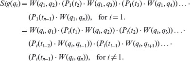
Example 5.32   We have seen earlier that gen-long-uio fails to generate a UIO sequence for state q₁ in M₂ shown in Figure 5.18. Let us therefore apply the method described above for the construction of a signature for state q₁. The desired signature can be found by substituting the appropriate values in the following formula.

Sig(q₁) = W(q₁, q₂) · (P₁(t₁) · W(q₁, q₃))

From Example 5.30, we have the following distinguishing sequences for state q₁.

W(q₁, q₂) = a/0

W(q₁, q₃) = b/0

The application of W(q₁, q₂) to state q₁ takes M₂ to state q₂. Hence we need the transfer sequence P₁(q₂) to bring M₂ back to state q₁. From Example 5.31 we get P₁(q₂) = a/1. Substituting these values in the formula for Sig(q₁), we obtain the desired signature.

 

Sig(q₁) = a/0 · a/1 · b/0

 

Later, while deriving test cases from UIO of different states, we will use signatures for states that do not possess a UIO.

5.8.7  Test generation

Let Μ = (X, Y, Q, q₁, δ, O) be an FSM from which we need to generate tests to test an implementation for conformance. Let Ε denote the set of core edges in M. m is the total number of core edges in M. Recall that edges corresponding to a reset input in each state are included in E. The following procedure is used to construct a total of m tests, each corresponding to the tour of an edge.

 

1. Find the UIO for each state in M.
2. Find the shortest path from the initial state to each of the remaining states. As before, the shortest path from the initial state q₁ to any other state q_i ∈ Q is denoted by P_i(q₁).
3. Construct an edge tour for each edge in M. Let TE(e) denote a subsequence that generates a tour for edge e. TE(e) is constructed as follows

    

   TE(e) = P_head(e)(1) · label(e) · UIO(tail(e)).

    

4. This step is optional. It is used to combine the Μ test subsequences generated in the previous step into one test sequence that generates the tour of all edges. This sequence is denoted by ΤA. It is sometimes referred to as β-sequence. TA is obtained by catenating pairs of reset input and edge tour subsequences as follows

   TA = X_e∈E((Re/null) · TE(e)).

TA is useful when the IUT can be brought automatically to its start state by applying an Re. In this case, the application of TA will likely shorten the time to test the IUT. While testing an IUT, the application of Re might be possible automatically through a script that sends a “kill process” signal to terminate the IUT and, upon the receipt of an acknowledgment that the process has terminated, may restart the IUT for the next test.

The next example illustrates the test generation procedure using the UIO sequences generated from M₁ shown in Figure 5.18.

 

Example 5.33   The UIO sequences for each of the six states in M₁ are reproduced below for convenience. Also included in the rightmost column are the shortest paths from state q₁ to the state corresponding to the state in the leftmost column.

State(s)	UIO (s)	Pi(q1)
q1 q2 q3 q4 q5 q6	a/0· c/1 c/1· c/1 b/1· b/1 b/1· c/0 c/0 c/1· a/0	null a/0 a/0· a/0 a/0· a/0· a/0 a/0· a/0· a/0· b/1 a/0· c/1

We consider only the core edges while developing tests for each edge. For example, the self-loop in state q₅ corresponding to inputs a and b, not shown in Figure 5.18, is ignored as it is not part of the core behavior of M₁. Also note that edge (q₆, q₁) will be considered twice, one corresponding to the label c/0 and the other corresponding to label Re/null. Using the formula given above, we obtain the following tests for each of the 14 core edges.

Test count	Edge (e)	TE(e)
1 2 3 4 5 6 7 8 9 10 11 12 13 14	q1, q2 q1, q1 q2, q3 q2, q6 q2, q1 q3, q4 q3, q4 q3, q1 q4, q5 q4, q1 q5, q6 q5, q1 q6, q1 q6, q1	a/0· c/1· c/1 Re/null/· Re/null/· a/0· c/1 a/0· a/0· b/1· b/1 a/0· c/1· c/1· a/0 a/0· Re/null· a/0· c/1 a/0· a/0· a/0· b/1· c/0 a/0· a/0· b/1· b/1· c/0 a/0· a/0· Re/null· a/0· c/1 a/0· a/0· a/0· c/0 a/0· a/0· a/0· Re/null· a/0· c/1 a/0· a/0· b/1· c/0· c/1 a/0· a/0· a/0· b/1· Re/null· a/0· c/1 a/0· c/1· c/1· a/0· c/1 a/0· c/1· Re/null· a/0· c/1

The 14 tests derived above can be combined into a β-sequence and applied to the IUT. This sequence will exercise only the core edges. Thus, for example, the self-loops in state q₅, corresponding to inputs a and b will not be exercised by the tests given above. It is also important to note that each TE(e) subsequence is applied with the IUT in its start state implying that a Re input is applied to the IUT prior to exercising it with the input portion of TE(e).

5.8.8  Test optimization

The set of test subsequences TE(e) can often be reduced by doing a simple optimization. For example, if TE(e₁) is a subsequence of test TE(e₂), then ΤΕ(e₁) is redundant. This is because the edges toured by ΤΕ(e₁) are also toured by TE(e₂), and in the same order. Identification and elimination of subsequences that are fully contained in another subsequence generally leads to a reduction in the size of the test suite. In addition, if two tests are identical, then one of them can be removed from further consideration. (See Exercise 5.21.)

 

Example 5.34   In an attempt to reduce the size of the test set derived in Example 5.33, we examine each test and check if it is contained in any of the remaining tests. We find that test 3 is fully contained in test 7, test 1 is contained in test 4, and test 4 is contained in test 13. Thus, the reduced set of tests consists of 11 tests: 2, 5, 6, 7, 8, 9, 10, 11, 12, 13, and 14 given in Example 5.33.

The tests derived in Example 5.33 are useful for a weak conformance test. To perform a strong conformance test of the IUT against the specification, we need to derive tests for non-core edges as well. The method for deriving such tests is the same as that given earlier for deriving TE(e) for the tour of edge e except that e now includes non-core edges.

 

Example 5.35   We continue Example 5.33for M₁ and derive additional tests needed for strong conformance. To do so, we need to identify the non-core edges. There are 10 non-core edges corresponding to the six states. Figure 5.21 shows the state diagram of M₁ with both core and non-core edges shown. Tests that tour the non-core edges can be generated easily using the formula for TE given earlier. The 10 tests follow.

 

Test count	Edge (e)	TE(e)
1 2 3 4 5 6 7 8 9 10	(q1, q1)b/null (q1, q1)c/null (q2, q2)b/null (q3, q3)c/null (q4, q4)a/null (q4, q4)c/null (q5, q5)a/null (q5, q5)b/null (q6, q6)a/null (q6, q6)b/null	b/null· a/0· c/1 c/null· a/0· c/1 a/0· b/null· c/1· c/1 a/0· a/0· c/null· b/1· b/1 a/0· a/0· a/0· a/null· b/1· c/0 a/0· a/0· a/0· c/null· b/1· c/0 a/0· a/0· a/0· b/1· a/null· c/0 a/0· a/0· a/0· b/1· b/null· c/0 a/0· c/1· a/null· c/1· a/0 a/0· c/1· b/null· c/1· a/0

Figure 5.21 Machine Μ₁, from Figure 5.18 with all non-core edges shown as dashed lines.

Note that a test for non-core edge e is similar to the tests for core edges in that the test first moves the machine to head(e). It then traverses the edge itself. Finally, it applies UIO(tail(e)) starting at state tail(e). Thus, in all, we have 21 tests to check for strong conformance of an IUT against M.

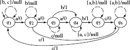
5.8.9  Fault detection

Tests generated using the UIO sequences are able to detect all operation and transfer errors. However, combination faults, such as an operation error and a transfer error might not be detectable. The next two examples illustrate the fault detection ability of the UIO method.

 

Example 5.36   Consider the transition diagram in Figure 5.22. Suppose that this diagram represents the state transitions in an IUT to be tested for strong conformance against machine M₁ in Figure 5.21. The IUT has two errors. State q₂ has a transfer error due to which δ(q₂, c) = q₅ instead of δ(q₂, c) = q₆. State q₃ has an operation error due to which O(q₃, b) is undefined.

Figure 5.22 State diagram of an IUT containing two faults. State q₂ has a transfer error and q₃ has an operation error. The behavior of this IUT is to be tested against that of the machine in Figure 5.21. Non-core edges are not shown.

To test the IUT against its specification as in Figure 5.21, one needs to apply the β sequence to the IUT and observe its behavior. The β sequence is obtained by combining all subsequences derived for weak and strong conformance in the earlier examples. However, as such a β sequence is too long to be presented here, we use an alternate method to show how the faults will be detected.

First, consider the transfer error in state q₂. Let us apply the input portion of test 4, which is TE(q₂, q₆), to the IUT. We assume that the IUT is in its start state, i.e. q₁, prior to the application of the test. From Example 5.33, we obtain the input portion as acca. The expected behavior of the IUT for this input is determined by tracing the behavior of the machine in Figure 5.21. Such a trace gives us O(q₁, acca) = 0110. However, when the same input is applied to the IUT, we obtain O(q₁, acca) = 010null.

As the IUT behaves differently than its specification, TE(q₂, q₆) has been able to discover the fault. Note that if test 4 has been excluded due to optimization, then test 13 can be used instead. In this case, the expected behavior is O(q₁, accac) = 01101, whereas the IUT generates O(q₁, accac) = 010null1 which also reveals a fault in the IUT.

Next, let us consider the operation error in state q₃ along the edge (q₃, q₄)_c/1. We use test 7. The input portion of this test is aabbc. For the specification, we have O(q₁, aabbc) = 00110. Assuming that this test is applied to the IUT in its start state, we get O(q₁, aabbc) = 00nullnull1 which is different from the expected output and thus test 7 has revealed the operation fault. (Also see Exercise 5.10.)

 

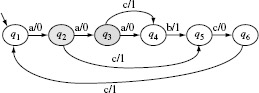
Example 5.37   Consider the specification shown in Figure 5.23(a). We want to check if tests generated using the UIO method will be able to reveal the transfer error in the IUT shown in Figure 5.23(b). UIO sequences and shortest paths from the start state to the remaining two states are given below.

 

State(s)	UIO (s)	Pi(q1)
q1 q2 q3	a/1 a/0· a/1 b/1· a/1 (also a/0· a/0)	null a/0 b/1

Figure 5.23 State diagram of an FSM for which a test sequence derived using the UIO approach does not reveal the error. (a) Specification FSM. (b) State diagram of a faulty IUT.

Given below are tests for touring each of the nine core edges including three edges that bring each state to state q₁ upon reset. Notice that we have added the Re/null transition at the start of each test sequence to indicate explicitly that the machine starts in state q₁ prior to the test being applied.

Test count	Edge (e)	TE(e)
Edges (e) from each state to state q1, label(e) = Re/null
1	q1, q1	Re/null· Re/null· a/1
2	q2, q1	Re/null· a/1Re/null· a/1
3	q3, q1	Re/null· b/1· Re/null· a/1
Edges shown in Figure 5.23(a)
4	q1, q2	Re/null· a/1· a/0· a/1
5	q1, q3	Re/null· b/1· b/1· a/1
6	q2, q1	Re/null· a/1· a/0· a/1
7	q2, q3	Re/null· a/1· b/1· b/1· a/1
8	q3, q1	Re/null· b/1· b/1· a/1
9	q3, q2	Re/null· b/1· a/0· a/0· a/1

To test the IUT let us apply the input portion bba of test 5 that tours the edge (q₁, q₃). The expected output is 111. The output generated by the IUT is also 111. Hence, the tour of edge (q₁, q₃) fails to reveal the transfer error in state q₁. However, test 9 that tours edge (q₃, q₂) does reveal the error because the IUT generates the output 1101, whereas the expected output is 1001, ignoring the null output. Note that tests 4 and 6 are identical and so are tests 5 and 8. Thus, an optimal test sequence for this example is the set containing tests 1, 2, 3, 4, 5, 7, and 9.

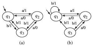
5.9  Automata Theoretic Versus Control-Flow Based Techniques

The test generation techniques described in this chapter fall under the automata theoretic category. There exist other techniques that fall under the control-flow based category. Here, we compare the fault detection effectiveness of some techniques in the two categories.

Several empirical studies have aimed at assessing the fault detection effectiveness of test sequences generated from FSMs by various test generation methods. Here we compare the fault detection effectiveness of the W and Wp-methods with four control-flow based criteria to assess the adequacy of tests. Some of the control theoretic can be applied to assess the adequacy of tests derived from FSMs against the FSM itself. In this section, we define four such criteria and show that tests derived from the W- and Wp-methods are superior in terms of their fault detection effectiveness than the four control-flow based methods considered.

Tests generated using the W- and Wp-methods guarantee the detection of all missing transitions, incorrect transitions, extra or missing states, and errors in the output associated with a transition given that the underlying assumptions listed in Section 5.6.1 hold. We show through an example that tests generated using these methods are more effective in detecting faults than the tests that are found adequate with respect to state cover, branch cover, switch cover, and the boundary interior cover test adequacy criteria. First, a few definitions before we illustrate this fact.

State cover:

A test set Τ is considered adequate with respect to the state cover criterion for an FSM Μ if the execution of Μ against each element of Τ causes each state in Μ to be visited at least once.

 

Transition cover:

A test set Τ is considered adequate with respect to the branch, or transition, cover criterion for an FSM Μ if the execution of Μ against each element of Τ causes each transition in Μ to be taken at least once.

Switch cover:

A test set Τ is considered adequate with respect to the 1-switch cover criterion for an FSM Μ if the execution of Μ against each element of Τ causes each pair of transitions (tr₁, tr₂) in Μ to be taken at least once, where for some input substring ab ∈ X*, tr₁ : q_i = δ(q_j, a) and tr₂ : q_k = δ(q_i, b) and q_i, q_j, q_k are states in M.

Boundary-interior cover:

A test set Τ is considered adequate with respect to the boundary-interior cover criterion for an FSM Μ if the execution of Μ against each element of Τ causes each loop body to be traversed zero times and at least once. Exiting the loop upon arrival covers the “boundary” condition and entering it and traversing the body at least once covers the “interior” condition.

The next example illustrates weaknesses of the state cover, branch cover, switch cover, and the boundary interior cover test adequacy criteria.

 

Example 5.38   This example is due to T.S. Chow. Machine M₁ in Figure 5.24 represents the correct design while M′₁ has an operation and a transfer error in state q₂. Note that M₁ has two states and four transitions.

Figure 5.24 Machine M′₁ contains a transfer fault with respect to machine M₁ in state q₂.

Consider the input sequence t = aabb. t covers all states and transitions in M₁ and hence is adequate with respect to the state coverage and transition coverage criteria. We obtain δ_M1(q_l, t) = 0111 and δ_M1′(q_l, t) = 0100. Thus, the operation error is detected but not the transfer error.

Next, consider machine M₂ in Figure 5.25 that represents correct design while M′₂ has a transfer error in state q₃. In order for a test set to be adequate with respect to the switch cover criterion, it must cause the following set of branch pairs to be exercised.

Figure 5.25 Machine M′₂ contains a transfer fault with respect to machine M₂ in state q₃.

The following table lists a set of test sequences adequate with respect to the switch cover criterion but do not reveal the transfer error in state q₃. The second column in the table shows the output generated and the rightmost column lists the switches covered.

Test sequence (t)	OM2(q1,t)(=OM′2(q1, t))	Switches covered
abbaaab   aaba aabb baab bb	0111001   0110 0110 0001 01	(tr1, tr2), (tr2, tr2), (tr2, tr3), (tr3, tr4), (tr4, tr4), (tr4, tr5) (tr1, tr3), (tr3, tr5), (tr5, tr1) (tr1, tr3), (tr3, tr5), (tr5, tr6) (tr6, tr4), (tr4, tr4), (tr4, tr5) (tr6, tr5)

A simple inspection of machine M₂ in Figure 5.25 reveals that all states are 1-distinguishable, i.e. for each pair of states (q_i, q_j), there exists a string of length 1 that distinguishes q_i from q_j, 1 ≤ (i, j) ≤ 3, i ≠ j. Later we define an n-switch cover and show how to construct one that reveals all transfer and operation errors for an FSM that is n-distinguishable.

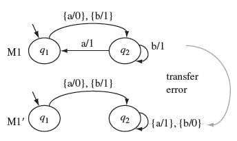
5.9.1  n-switch-cover

The switch-cover criterion can be generalized to an n-switch cover criterion as follows. An n-switch is a sequence of (n + 1) transitions. For example, for machine M₃ in Figure 5.26, transition sequence tr₁ is a 0-switch, tr₁, tr₂ is a 1-switch, tr₁, tr₂, tr₃ is a 2-switch, and transition sequence tr₆, tr₅, tr₁, tr₃ is a 3-switch. For a given integer n > 0, we can define an n-switch set for a transition tr as the set of all n-switches with tr as the prefix. For example, for each of the six transitions in Figure 5.26, we have the following 1-switch sets.

 

tr₁ : {(tr₁, tr₂), (tr₁, tr₃)}

tr₂ : {(tr₂, tr₂), (tr₂, tr₃)}

tr₃ : {(tr₃, tr₄), (tr₃, tr₅)}

tr₄ : {(tr₄, tr₄), (tr₄, tr₅)}

tr₅ : {(tr₅, tr₆), (tr₅, tr₁)}

tr₆ : {(tr₆, tr₄), (tr₆, tr₅)}

  

Figure 5.26 Machine M′₃ contains a transfer fault with respect to machine M₃ in state q₂.

An n-switch set S for a transition tr in FSM Μ is considered covered by a set Τ of test sequences if exercising Μ against elements of Τ causes each transition sequence in S to be traversed. Τ is considered an n-switch set cover, if it covers all n-switch sets for FSM M. It can be shown that an n-switch set cover can detect all transfer, operation, extra, and missing state errors in a minimal FSM that is n-distinguishable (see Exercise 5.28). Given a minimal, 1-distinguishable FSM M, the next example demonstrates a procedure to obtain a 1-switch cover using the testing tree of M.

 

Example 5.39   Figure 5.27 shows a testing tree for machine M₃ in Figure 5.26. To obtain the 1-switch cover, we traverse the testing tree from the root and enumerate all complete paths. Each path is represented by the sequence s of input symbols that label the corresponding links in the tree. The sequence s corresponding to each path is concatenated with the input alphabet of Μ as s.x where x ∈ Χ, X being the input alphabet. Traversing the testing tree in Figure 5.27 and concatenating as described gives us the following 1-switch cover.

 

Τ = {aba, abb, aaa, aab, baa, bab, bba, bbb}

Figure 5.27 Testing tree of machine M₃ in Figure 5.26.

We leave it to you to verify that T is a 1-switch cover for M₃. Note that test aba ∈ Τ distinguishes M₃ from M′₃ as O_M3(q₁, abb) = 000 ≠ O_M′3(q₁, abb). Exercise 5.30 asks for the derivation of a test set from M₂ in Figure 5.25 that is adequate with respect to 1-switch cover criterion.

5.9.2  Comparing automata theoretic methods

Figure 5.28 shows the relative fault detection effectiveness of the transition tour (TT), Unique Input/Output (UIO), UIOv, Distinguishing Sequence (DS) Wp-, and W-methods. As is shown in the figure, the W-method, UIOv, Wp, and DS can detect all faults using the fault model described in Section 5.4.

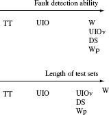
Figure 5.28 Relative fault detection effectiveness and length of the test sets of various automata theoretic techniques.

The distinguishing sequence method constructs an input sequence x from an FSM Μ such that O(q_i, x) is different for each q_iin M. Sequences so constructed are able to detect all faults in our fault model. The UIO method is able to detect all output faults along transitions but not necessarily all transfer faults.

Note that the transition tour method has the lowest fault detection capability. In this method, test sequences are generated randomly until all transitions in the underlying FSM are covered. Redundant sequences are removed using a minimization procedure. One reason for the low fault detection ability of the TT method is that it checks only whether or not a transition has been covered and does not check the correctness of the start and tail states of the transition (see Exercise 5.25).

 

The relative lengths of test sequences is shown in Figure 5.28. Once again the W-method generates the longest, and the largest, set of test sequences while the TT method the shortest. From the relative lengths and fault detection relationships, we observe that larger tests tend to be more powerful than shorter tests. However, we also observe that smaller tests can be as powerful in their fault detection ability as the larger tests as indicated by comparing the fault detection effectiveness of the Wp- with that of the W-method.

 

5.10  Tools

There are only a few freely available tools for generating tests from finite state models. However, a number of commercial tools are available that enable the tasks of model specification, exploration, and test generation. Some are mentioned below.

Spec Explorer: This tool from Microsoft is a giant in terms of what it offers to a tester. It allows the representation of a meta state model in Spec# and Asml languages that are based on C#. This model is an expression of the program’s intended behavior. What a program must do and what it must not do are specified in the Spec# model. The model need not express all of a program’s intended behavior. Instead, one may create several models from different points of views. From the model, the tool generates a number of FSMs that sample the program’s behavior. Tests are generated from each machine.

Documentation and link: http://research.microsoft.com/en-us/projects/specexplorer/

T-UPPAAL: This is a powerful tool for testing embedded real-time systems. The input to T-UPPAAL is a model of the system under test as a timed automata. Using this formal model, T-UPPAAL generates and executes timed test sequences.

Documentation and link: http://people.cs.aau.dk/~marius/tuppaal/

 

ModelJUnit: This is a Java library that extends JUnit. An FSM or EFSM model is specified as a set of Java classes. Tests are generated from these models.

Documentation and link: http://czt.sourceforge.net/modeljunit/index.html

WMethod: This is an easy-to-use tool to generate tests from an FSM. It takes an FSM as input and generates tests using the W-method described in this chapter.

Documentation and link: http://www.cs.purdue.edu/homes/apm/foundationsBook/

 

Exercises

5.1 Modify the DIGDEC machine shown in Figure 5.3 so that it accepts a string over the alphabet X = {d, *}. For example, strings such as s = 324*41*9*199**230* are valid inputs. An asterisk causes the machine to execute the OUT(num) function where num denotes the decimal number corresponding to the digits received prior to the current asterisk but after any previous asterisk. Thus, the output of the machine for input string s will be

OUT(324) OUT(41) OUT(9) OUT(199) OUT(230)

Notice that the machine does not perform any action if it receives an asterisk following another asterisk.

5.2 Show that (a) V-equivalence and equivalence of states and machines as defined in Section 5.2.3 are equivalence relations, i.e. they obey the reflexive, symmetric, and transitive laws; (b) if two states are k-distinguishable for any k > 0, then they are also distinguishable for any n ≥ k.

5.3 Show that it is not necessary for equivalent machines to have an equal number of states.

5.4 Show that the set W of Example 5.7 is a characterization set for the machine in Figure 5.13.

5.5 Prove that the FSM Μ must be a minimal machine for the existence of a characterization set.

5.6 Prove that the method for the construction of k-equivalence partitions described in Example 5.8 will always converge, i.e. there will be a table P_n, n > 0, such that P_n = P_n+1.

5.7 The W-procedure for the construction of the W-set from a set of k-equivalence partitions is given on page 239. This is a brute force procedure that determines a distinguishing sequence for every pair of states. From Example 5.9, we know that two or more pairs of states might be distinguishable by the same input sequence. Rewrite the W-procedure by making use of this fact.

5.8 Prove that the k-equivalence partition of a machine is unique.

5.9 Prove that in an FSM with n states, at most n – 1 constructions of the equivalence classes are needed, i.e. one needs to construct only P₁, P₂, ...,P_n–1.

5.10 Given the FSM of Example 5.6, construct all mutants that can be obtained by adding a state to M.

5.11 Generate a set Τ of input sequences that distinguish all mutants in Figure 5.12 from machine M.

5.12 Show that any extra or missing state error in the implementation of design Μ will be detected by at least one test generated using the W-method.

5.13 Construct the characterization set W and the transition cover for the machine in Figure 5.23(a). Using the W-method, construct set Ζ assuming that m = 3 and derive a test set Τ. Does any element of Τ reveal the transfer error in the IUT of Figure 5.23(b)? Compare Τ with the test set in Example 5.37 with respect to the number of tests and the average size of test sequences.

5.14 Consider the design specification Μ as shown in Figure 5.15(a). Further, consider an implementation M₃ of Μ as shown in Figure 5.29. Find all tests in T₁ and T₂ from Example 5.17 that reveal the error in M₃.

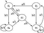
Figure 5.29 An implementation of Μ shown Figure 5.15(a) with a transfer error in state q₁, on input a.

5.15 Consider the design specification in Figure 5.30(a). It contains three states q₀, q₁, and q₂. The input alphabet X = {a, b, c}, and the output alphabet is Y = {0, 1}. (a) Derive a transition cover set P, the state cover set S, the characterization set W, and state identification sets for each of the three states. (b) From M, derive a test set T_w using the W-method and test set T_wp using the Wp-method. Compare the sizes of the two sets, (c) Figure 5.30(b) shows the transition diagram of an implementation of Μ that contains a transfer error in state q₂. Which tests in T_w and T_wp reveal this error? (d) Figure 5.30(c) shows the transition diagram of an implementation of Μ that contains an extra state q₃, and a transfer error in state q₂. Which tests in T_w and T_wp reveal this error ?

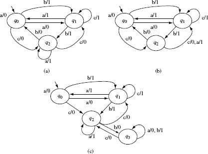
Figure 5.30 Three FSMs. (a) Design specification machine, (b) and (c) are machine indicating an erroneous implementation of the FSM in (a).

5.16 (a) Given an FSM Μ = (Χ, Y, Q, q₀, δ, O) where |X| = n_x, |Y| = n_y, |Q| = n_z, calculate the upper bound on the number of tests that will be generated using the W-method. (b) Under what condition(s) will the number of tests generated by the Wp-method be the same as those generated by the W-method?

5.17 Using the tests generated in Example 5.18, determine at least one test for each of the two machines in Figure 5.16 that will reveal the error. Is it necessary to apply phase 2 testing to reveal the error in each of the two machines ?

5.18 What is the difference between sequences in the W set and the UIO sequences ? Find UIO sequences for each state in the machine with transition diagram shown in Figure 5.13. Find the distinguishing signature for states for which a UIO sequence does not exist.

5.19 What will be the value of counter k when control arrives at Step 2.3 in procedure gen-long-uio?

5.20 For machine M₂ used in Example 5.32, what output sequences are generated when the input portion of Sig(q₁) is applied to states q₂ and q₃?

5.21 Suppose that tests ΤΕ(e₁) and TE(e₂) are derived using the method in Section 5.8.7 for a given FSM M. Is it possible that TE(e_l) = TE(e₂)?

5.22 Generate UIO sequences for all states in the specification shown in Figure 5.13. Using the sequences so generated, develop tests for weak conformance testing of an IUT built that must behave as per the specification given.

5.23 Generate tests for weak conformance testing of machine M₂ in Figure 5.18. Use the UIO sequences for M₂ given on page 259.

5.24 Consider an implementation of the machine shown in Figure 5.21. The state diagram of the implementation is shown in Figure 5.31. Note that the IUT has two errors, a transfer error in state q₂ and an operation error in state q₆. In Example 5.36, the transfer error in q₂ is revealed by test 4 (and 13). Are any of these tests successful in revealing the error in q₂ ? Is there any test derived earlier that will reveal the error in q₂ ? Which one of the tests derived in Example 5.33 and 5.35 will reveal the error in q₆ ?

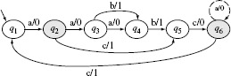
Figure 5.31 State diagram of an erroneous implementation of the machine in Figure 5.21.

5.25 Transition tours is a technique to generate tests from specification FSMs. A transition tour is an input sequence that when applied to an FSM in its start state traverses each edge at least once. (a) Find a transition tour for each of the two FSMs shown in Figure 5.18. (b) Show that a transition tour is able to detect all operation errors but may not be able to detect all transfer errors. Assume that the FSM specification satisfies the assumptions in Section 5.6.1. (c) Compare the size of tests generated using transition tours and the W-method.

5.26 In Example 5.38, we developed adequate tests to show that certain errors in the IUT are not detected. Derive tests using the W-method, and then using the Wp-method, and show that each test set derived detects all errors shown in Figure 5.32.

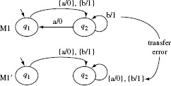
Figure 5.32 A transfer error.

5.27 FSM models considered in this chapter are pure in the sense that they capture only the control flow and ignore data definitions and uses. In this exercise, you will learn how to enhance a test set derived using any of the methods described in this chapter by accounting for data flows.

Figure 5.33 shows machine M, an augmented version of the FSM in Figure 5.13. We assume that the IUT corresponding to the FSM in Figure 5.33 uses a local variable Z. This variable is defined along transitions tr₁ = (q₁, q₄) and tr₃ = (q₃, q₅). Variable Ζ is used along transitions tr₂ = (q₂, q₁) and tr₄ = (q₃, q₁). Also, x and y are parameters of, respectively, inputs b and a. A data flow path for variable Ζ is a sequence Tr of transitions such that Ζ is defined on one transition along Tr and subsequently used along another transition also in Tr. For example, tr₁, tr₅, tr₄ is a data flow path for Ζ in M, where Ζ is defined along tr₁ and used along tr₄. We consider only finite length paths and those with only one definition and one corresponding use along a path.

While testing the IUT against M, we must ensure that all data flow paths are tested. This is to detect faults in the defining or usage transitions. (a) Enumerate all data flow paths for variable Ζ in M. (b) Derive tests, i.e. input sequences, that will traverse all data flow paths derived in (a). (c) Consider a test set Τ derived for Μ using the W-method. Does exercising Μ against all elements of Τ exercise all data flow paths derived in (a) ? (Note: Chapter 7 provides details of data-flow based assessment of test adequacy and enhancement of tests.)

Figure 5.33 FSM of Figure 5.13 augmented with definition and use of local variable Z.

5.28 Let T be a set of test inputs that forms an n-switch set cover for a minimal n-distinguishable FSM M. Prove that Τ can detect all transfer, operation, extra, and missing state errors in M.

5.29 Show that a test set Τ that is adequate with respect to the boundary-interior coverage criterion may not be adequate with respect to the 1-switch cover criterion.

5.30 Derive a test set Τ from M₂ shown in Figure 5.25 that is adequate with respect to the 1-switch cover criterion. Which test in Τ distinguishes M₂ from M′₂ and thereby reveals the error ? Compare Τ derived in this exercise with the test given in Example 5.38 and identify a property of the method used to construct Τ that allows Τ to distinguish M₂ from M′₂.