8

Test Adequacy Assessment using Program Mutation

The purpose of this chapter is to introduce Program Mutation as a technique for the assessment of test adequacy and the enhancement of test sets. The chapter also focuses on the design and use of mutation operators for procedural and objected-oriented programming languages.

8.1  Introduction

Program mutation is a powerful technique for the assessment of the goodness of tests. It provides a set of strong criteria for test assessment and enhancement. If your tests are adequate with respect to some other adequacy criterion, such as the modified condition/decision coverage (MC/DC) criterion, then chances are that these are not adequate with respect to most criteria offered by program mutation.

 

Program mutation is a technique to assess and enhance your tests. Hereafter we will refer to “program mutation” as “mutation.” When testers use mutation to assess the adequacy of their tests, and possibly enhance them, we say that they are using mutation testing. Sometimes the act of assessing test adequacy using mutation is also referred to as mutation analysis.

 

Given that mutation requires access to all or portions of the source code, it is considered as a white-box, or code-based, technique. Some refer to mutation testing as fault injection testing. However, it must be noted that fault-injection testing is a separate area in its own right and must be distinguished from mutation testing as a technique for test adequacy and enhancement.

Mutation has also been used as a black-box technique. In this case, it is used to mutate specifications and, in the case of web applications, messages that flow between a client and a server. This chapter focuses on the mutation of computer programs written in high-level languages such as Fortran, C, and Java.

While mutation of computer programs requires access to the source code of the application under test, some variants can do without. Interface mutation requires access only to the interface of the application under test. Run-time fault injection, a technique similar to mutation, requires only the binary version of the application under test.

Mutation can be used to assess and enhance tests for program units, such as C functions and Java classes. It can also be used to assess and enhance tests for an integrated set of components. Thus, as explained in the remainder of this chapter, mutation is a powerful technique for use during unit, integration, and system testing.

 

A cautionary note: Mutation is a significantly different way of assessing test adequacy than what we have discussed in the previous chapters. Thus, while reading this chapter, you will likely have questions of the kind “Why this …” or “Why that …” With patience, you will find that most, if not all, of your questions are answered in this chapter.

8.2  Mutation and Mutants

Mutation is the act of changing a program, albeit only slightly. If Ρ denotes the original program under test and Μ a program obtained by slightly changing P, then Μ is known as a mutant of Ρ and Ρ the parent of M. Given that Ρ is syntactically correct, and hence compiles, Μ must be syntactically correct. Μ might or might not exhibit the behavior of Ρ from which it is derived.

 

The term “to mutate” refers to the act of mutation. To “mutate” a program means to change it. Of course, for the purpose of test assessment, we mutate by introducing only “slight” changes.

 

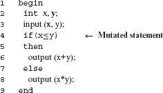
Example 8.1   Consider the following simple program.

Program P8.1

1 begin

2   int x, y;

3   input (x, y);

4   if (x<y)

5      output (x+y);

6   else

7      output (x*y);

8 end

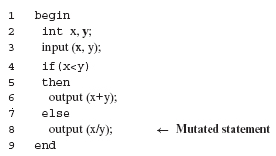
A large variety of changes can be made to P8.1 such that the resultant program is syntactically correct. Below we list two mutants of P8.1. Mutant M1 is obtained by replacing the < operator by the ≤ operator. Mutant M2 is obtained by replacing the * operator by the / operator.

Mutant M1 of Program P8.1

Mutant M2 of Program P8.1

Notice that the changes made in the original program are simple. For example, we have not added any chunk of code to the original program to generate a mutant. Also, only one change has been made to the parent to obtain its mutant.

8.2.1  First order and higher order mutants

Mutants generated by introducing only a single change to a program under test are also known as first order mutants. Second order mutants are created by making two simple changes, third order by making three simple changes, and so on. One can generate a second order mutant by creating a first order mutant of another first order mutant. Similarly, an nth order mutant can be created by creating a first order mutant of an (n – 1)^th order mutant.

 

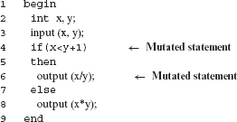
Example 8.2   Once again let us consider Program P8.1. We can obtain a second order mutant of this program in a variety of ways. Here is a second order mutant obtained by replacing variable y in the if statement by the expression y+1, and replacing operator + in the expression x+y by the operator /.

Mutant M3 of Program P8.1

Mutants, other than first order, are also known as higher order mutants. First order mutants are the ones generally used in practice. There are two reasons why first order mutants are preferred to higher order mutants. One reason is that there are many more higher order mutants of a program than first order mutants. For example, 528,906 second order mutants are generated for program FIND that contains only 28 lines of Fortran code. Such a large number of mutants create a scalability problem during adequacy assessment. Another reason has to do with the coupling effect and is explained in Section 8.6.2.

 

Note that so far we have used the term “simple change” without explaining what we mean by “simple” and what is a “complex” change. An answer to this question appears in the following sections.

8.2.2  Syntax and semantics of mutants

In the examples presented so far, we mutated a program by making simple syntactic changes. Can we mutate using semantic changes? Yes, we certainly can. However, note that syntax is the carrier of semantics in computer programs. Thus, given a program Ρ written in a well-defined programming language, a “semantic change” in Ρ is made by making one or more syntactic changes. A few illustrative examples follow.

 

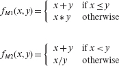
Example 8.3   Let f_P8.1(x, y) denote the function computed by Program P8.1. We can write f(x, y) as follows:

Let f_M1(x, y) and f_M2(x, y) denote the functions computed by M1 and M2, respectively. We can write f_M1(x, y) and f_M2(x, y) as follows:

Notice that the three functions f_P8.1(x, y), f_M1(x, y), and f_M2(x, y) are different. Thus, we have changed the semantics of P8.1 by changing its syntax.

The previous example illustrates the meaning of “syntax is the carrier of semantics.” Mutation might, at first thought, seem to be “just” a simple syntactic change made to a program. In effect, such a simple syntactic change could have a drastic effect, or it might have no effect at all, on program semantics. The next two examples illustrate why.

Example 8.4   Nuclear reactors are increasingly relying on the use of software for control. Despite the intensive use of safety mechanisms, such as the use of 400,000 liters of cool heavy water moderator, the control software must continually monitor various reactor parameters and respond appropriately to conditions that could lead to a meltdown. For example, the Darlington Nuclear Generating Station located near Toronto, Canada, uses two independent computer–based shutdown systems. Though formal methods can be, and have been, used to convince the regulatory organizations that the software is reliable, a thorough testing of such systems is inevitable.

 

Thorough testing of critical software systems is inevitable even after the software has been formally verified.

While the decision logic in a software-based emergency shutdown system would be quite complex, the highly simplified procedure below indicates that simple changes to a control program might lead to disastrous consequences. Assume that the checkTemp procedure is invoked by the reactor monitoring system with three most recent sensory readings of the reactor temperature. The procedure returns a danger signal to the caller through variable danger.

Program P8.2

1   enum dangerLevel {none, moderate, high, veryHigh};

2   procedure checkTemp (currentTemp, maxTemp) {

3     float currentTemp[3], maxTemp; int highCount=0;

4     enum dangerLevel danger;

5     danger=none;

6     if (currentTemp[0]>maxTemp)

7       highCount=1;

8     if (currentTemp[1]>maxTemp)

9       highCount=highCount+1;

10    if (currentTemp[2]) >maxTemp)

11      highCount=highCount+1;

12    if (highCount==1) danger=moderate;

13    if (highCount==2) danger=high;

14    if (highCount==3) danger=veryHigh;

15    return(danger);

16   }

 

Procedure checkTemp compares each of the three temperature readings against the maximum allowed. A “none” signal is returned if none of the three readings is above the maximum allowed. Otherwise, a “moderate,” “high,” or “veryHigh” signal is returned depending on, respectively, whether one, two, or three readings are above the allowable maximum. Now consider the following mutant of P8.2 obtained by replacing the constant “veryHigh” with another constant “none” at line 14.

Mutant M1 of Program P8.2

1   enum dangerLevel {none, moderate, high, veryHigh};

2   procedure checkTemp (currentTemp, maxTemp){

3     float currentTemp[3], maxTemp; int highCount=0;

4     enum dangerLevel danger;

5     danger=none;

6     if (currentTemp[0]>maxTemp)

7       highCount=1;

8     if (currentTemp[1]>maxTemp)

9       highCount=highCount+1;

10    if (currentTemp[2]) >maxTemp)

11      highCount=highCount+1;

12    if (highCount==1) danger=moderate;

13    if (highCount==2) danger=high;

14    if (highCount==3) danger=none; ← Mutated statement

15    return(danger);

16   }

 

A simple syntactic change in a critical software system may lead to a disastrous change in its run time behavior.

Notice the difference in the behaviors of P8.2 and M1. Program P8.2 returns “veryHigh” signal when all three temperature readings are higher than the maximum allowable, its mutant M1 returns the “none” signal under the same circumstances.

While the syntactic change made to the program is trivial, the resultant change in its behavior could lead to an incorrect operation of the reactor shutdown software potentially causing a major environmental and human disaster. It is such changes in behavior that we refer to as drastic. Indeed, the term “drastic” in the context of software testing often refers to the nature of the possible consequence of a program’s, or its mutant’s, behavior.

Example 8.5   While a simple change in a program might create a mutant whose behavior differs drastically from its parent, another mutant might behave exactly the same as the original program. Let us examine the following mutant obtained by replacing the == operator at line 12 in P8.2 by the ≥ operator.

Mutant M2 of Program P8.2

1   enum dangerLevel {none, moderate, high, veryHigh};

2   procedure checkTemp (currentTemp, maxTemp) {

3     float currentTemp[3], maxTemp; int highCount=0;

4     enum dangerLevel danger;

5     danger=none;

6     if (currentTemp[0]>maxTemp)

7       highCount=1;

8     if (currentTemp[1]>maxTemp)

9       highCount=highCount+1;

10    if (currentTemp[2]) >maxTemp)

11      highCount=highCount+1;

12    if (highCount≥1) danger=moderate; ← Mutated statement

13    if (highCount==2) danger=high;

14    if (highCount==3) danger=veryHigh;

15    return(danger) ;

16   }

 

It is easy to check that for all triples of input temperature values and the maximum allowable temperature, P8.2 and M2 will return the same value of danger. Certainly, during execution, M2 will exhibit a different behavior than that of P8.2. However, the values returned by both the program and its mutant will be identical.

 

The behavior of a program Ρ and its mutant Μ can be compared at different points during execution. In most practical applications of mutation testing the behavior compared by an examination the observable (external) outputs of Ρ and Μ during or at the end of execution.

As shown in the examples above, while a mutant might behave differently than its parent during execution, in mutation testing the behavior of the two entities are considered identical if they exhibit identical behaviors at the specified points of observation. Thus, when comparing the behavior of a mutant with its parent, one must be clear about what are the points of observation. This leads us to strong and weak mutations.

8.2.3  Strong and weak mutations

We mentioned earlier that a mutant is considered distinguished from its parent when the two behave differently. A natural question to ask is “At what point during program execution should the behaviors be observed ?” We deal with two kinds of observations external and internal. Suppose we decide to observe the behavior of a procedure soon after its termination. In this case we observe the return value, and any side effects in terms of changes to values of global variables and data files. We shall refer to this mode of observation as external.

 

An internal observation refers to the observation of the state of a program, and its mutant, during their respective executions. Internal observations could be done in a variety of ways that differ in where the program state is observed. One could observe at each state change, or at specific points in the program.

Strong mutation testing uses external observation. Thus, a mutant and its parent are allowed to run to completion at which point their respective outputs are compared. Weak mutation testing uses internal observation. It is possible that a mutant behaves similar to its parent under strong mutation but not under weak mutation.

Example 8.6   Suppose we decide to compare the behaviors of Program P8.2 and its mutant M2 using external observation. As mentioned in the previous example, we will notice no difference in the behaviors of the two programs as both return the same value of variable danger for all inputs.

Instead, suppose we decide to use internal observation to compare the behaviors of Program P8.2 and M2. Further, the state of each program is observed at the end of the execution of each source line. The states of the two programs will differ when observed soon after line 12 for the following input t:

For the inputs above, the states of P8.2 and M2 observed soon after the execution of the statement at line 12 are as follows:

	danger	highCount
P8.2	none	2
M2	moderate	2

A program and its mutant might be equivalent under strong mutation but not under weak mutation.

Note that while the inputs are also a part of a program’s state, we have excluded them from the table above as they do not change during the execution of the program and its mutant. The two states shown above are clearly different. However, in this example, the difference observed in the states of the program and its mutant does not effect their respective return values, which remain identical.

For all inputs, M2 behaves identically to its parent P8.2 under external observation. Hence, M2 is considered equivalent to P8.2 under strong mutation. However, as revealed in the table above, M2 is distinguishable from P8.2 by test case t. Thus, the two are not equivalent under weak mutation.

8.2.4  Why mutate?

It is natural to wonder why a program should be mutated. Before we answer this question, let us consider the following scenario likely to arise in practice.

 

Suppose you have developed a program, say, P. You have tested P. You found quite a few faults in Ρ during testing. You have fixed all these faults and have retested P. You have even made sure that your test set is adequate with respect to the MC/DC criterion. After all this tremendous effort you have put into testing P, you are now justifiably confident that Ρ is correct with respect to its requirements.

Happy and confident, you are about to release Ρ to another group within your company. At this juncture in the project, someone takes a look at your program and, pointing to a line in your source code, asks “Should this expression be

 

boundary<corner, or

 

boundary<corner+1 ?” ”

 

Scenarios such as the one above arise during informal discussions with colleagues, and also during formal code reviews. A programmer is encouraged to show why an alternate solution to a problem is not the correct, or a better, than the one selected. The alternate solution could lead to a program significantly different from the current one. It could also be a simple mutant as in the scenario above.

 

There are several ways a programmer could argue in favor of the existing solution such as boundary<corner in the scenario above. One way is to give a performance related argument that shows why the given solution is better than the alternate proposed in terms of the performance of the application.

Another way is to show that the current solution is correct and preferred, and the proposed alternate is incorrect or not preferred. If the proposed alternate is a mutant of the original solution, then the programmer needs to simply show that the mutant behaves differently than the current solution and is incorrect. This can be done by proposing a test case and showing that the current solution and the proposed solutions are different and the current solution is correct.

It is also possible that the proposed alternate is equivalent to the current solution. However, this needs to be shown for all possible inputs and requires a much stronger argument than the one used to show that the alternate solution is incorrect.

 

Mutation offers a systematic way of generating a number of scenarios similar to the one described above. It places the burden of proof on the tester, or the developer that the program under test is correct while the mutant created is indeed incorrect. As we show in the remainder of this chapter, testing using mutation often leads to the discovery of subtle flaws in the program under test. This discovery usually takes place when a tester tries to show that the mutant is an incorrect solution to the problem at hand.

8.3  Test Assessment Using Mutation

Now that we know what mutation is, and what mutants look like, let us understand how mutation is used for assessing the adequacy of a test set. The problem of test assessment using mutation can be stated as follows.

Let Ρ be a program under test, Τ a test set for P, and R the set of requirements that Ρ must meet. Suppose that Ρ has been tested against all tests in Τ and found to be correct with respect to R on each test case. We want to know how good is Τ ?

 

Mutation offers a way of answering the question stated above. As explained later in this section, given Ρ and T, a quantitative assessment of the goodness of Τ is obtained by computing a mutation score of Τ. Mutation score is a number between 0 and 1. A score of 1 means that Τ is adequate with respect to mutation. A score lower than 1 means that Τ is inadequate with respect to mutation. An inadequate test set can be enhanced by the addition of test cases that increase the mutation score.

8.3.1  A procedure for test adequacy assessment

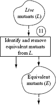
Let us now dive into a procedure for assessing the adequacy of a test set. One such procedure is illustrated in Figure 8.1. It is important to note that Figure 8.1 shows one possible sequence of 12 steps for assessing the adequacy of a given suite of tests using mutation; other sequencings are possible and discussed later in this section.

Do not be concerned if Figure 8.1 looks confusing and rather jumbled. Also, some terms used in the figure have not been defined yet. Any confusion should be easily overcome by going through the step-by-step explanation that follows. All terms used in the figure are defined as we proceed with the explanation of the assessment process.

For the sake of simplicity, we use Program P8.1 throughout our explanation through a series of examples. Certainly, P8.1 does not represent the kind of programs for which mutation is likely to be used in commercial and research environments. However, it serves our instructional purpose in this section: that of explaining various steps in Figure 8.1. Also, and again for simplicity, we assume that Program P8.1 is correct as per its requirements. In Section 8.8, we will see how the assessment of adequacy using mutation helps in the detection of faults in the program under test.

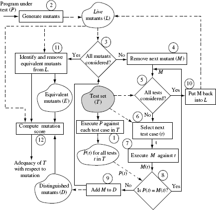
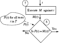
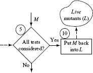
Figure 8.1 A procedure used in the assessment of the adequacy of a test set using mutation. Solid lines point to the next process step. Dashed lines indicate data transfer between a data repository and a process step. L, D, and Ε denote, respectively, the set of live, distinguished, and equivalent mutants defined in the text. P(t)and M(t)indicate, respectively, the program and mutant behaviors observed upon their execution against test case t.

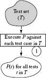
Step 1: Program execution

The first step in assessing the adequacy of a test set Τ with respect to program Ρ and requirements R, is to execute Ρ against each test case in Τ. Let P(t) denote the observed behavior of Ρ when executed against t. Generally, the observed behavior is expressed as a set of values of output variables in P. However, it might also relate to the performance of P.

This step might not be necessary if Ρ has already been executed against all elements in Τ and P(t) recorded in a database. In any case, the end result of executing Step 1 is a database of P(t) for all t ∈ Τ.

At this point we assume that P(t) is correct with respect to R for all t ∈ T. If P(t) is found to be incorrect, then Ρ must be corrected and Step 1 executed again. The point to be noted here is that test adequacy assessment using mutation begins when Ρ has been found to be correct with respect to the test set Τ.

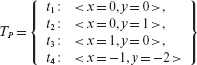
Example 8.7   Consider Program P8.1 which we shall refer to as P. Ρ is supposed to compute the following function f(x, y).

Suppose we have tested Ρ against the following set of tests.

The database of P(t) for all t ∈ T_P, is tabulated below.

Test case (t)	Expected output f (x, y)	Observed output P(t)
t1	0	0
t2	1	1
t3	0	0
t4	1	2

Note that P(t) computes function f(x, y), for all t ∈ T_P. Hence, the condition that P(t) be correct on all inputs from T_P, is satisfied. We can now proceed further with adequacy assessment.

 

Step 2: Mutant generation

The next step in test adequacy assessment is the generation of mutants. While we have shown what a mutant looks like and how it is generated, we have not given any systematic procedure to generate a set of mutants given a program. We will do so in Section 8.4.

 

For now we assume that the following mutants have been generated from Ρ by (a) altering the arithmetic operators such that any occurrence of the addition operator (+) is replaced by the subtraction operator (–) and that of the multiplication operator (*) by the divide operator (/), and (b) replacing each occurrence of an integer variable ν by ν + 1.

 

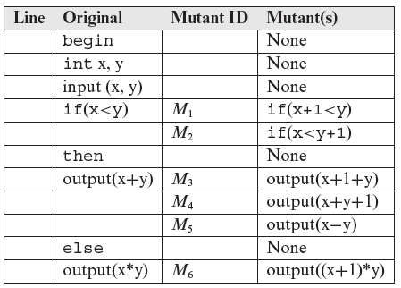
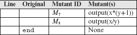
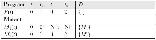
Example 8.8   By mutating the program as mentioned above, we obtain a total of eight mutants, labeled M₁ through M₈, shown in the following table. Note that we have not listed the complete mutant programs for the sake of saving space. A typical mutant will look just like Program P8.1 with one of the statements replaced by the mutant in the table below.

In the table above, notice that we have not mutated the declaration, input, then, and else statements. The reason for not mutating these statements is given later in Section 8.4. Of course, markers begin and end are not mutated.

At the end of Step 2, we have a set of eight mutants. We refer to these eight mutants as live mutants. These mutants are live because we have not yet distinguished them, from the original program. We will make an attempt to do so in the next few steps. Thus we obtain the set L = {M₁, M₂, M₃, M₄, M₅, M₆, M₇, M₈}. Note that distinguishing a mutant from its parent is sometimes referred to as killing a mutant.

 

Steps 3 and 4: Select next mutant

 

In Steps 3 and 4 we select the next mutant to be considered. This mutant must not have been selected earlier. Notice that at this point we are starting a loop that will cycle through all mutants in L until each mutant has been selected. Obviously, we select the next mutant only if there is a mutant remaining in L. This check is made in Step 3. If there are live mutants in L that have never been selected in any previous step, then a mutant is selected arbitrarily. The selected mutant is removed from L.

 

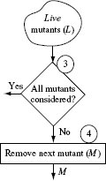
Example 8.9   In Step 3 eight mutants remain in L and hence we move to Step 4 and select any one of these eight. The choice of which mutant to select is arbitrary. Hence, let us select mutant M₁. After moving M₁ from L, we have L = {M₂, M₃, M₄, M₅, M₆, M₇, M₈}

 

Steps 5 and 6: Select next test case

 

Having selected a mutant M, we now attempt to find whether or not at least one of the tests in Τ can distinguish it from its parent P. To do so, we need to execute Μ against tests in Τ. Thus at this point we enter another loop that is executed for each selected mutant. The loop terminates when all tests are exhausted, or Μ is distinguished by some test, whichever happens earlier.

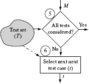
Example 8.10   Now that we have selected M₁, we need to check if can be distinguished by Τ from P. In Step 5 we select the next test. Again, any of the tests in T_P, against which M₁ has not been executed so far, can be selected. Let us select t₁: < x = 0, y = 0 >.

 

A mutant whose behavior is observed to be different from its parent program is considered “distinguished.” It is removed from further consideration.

Steps 7, 8, and 9: Mutant execution and classification

 

So far we have selected a mutant Μ for execution against test case t. In Step 7 we execute the Μ against t. In Step 8 we check if the output generated by executing Μ against t is the same or different from that generated by executing Ρ against t.

Example 8.11   So far we have selected mutant M₁ and test case t₁. In Step 7 we execute M₁ against t₁. Given the inputs x = 0 and y = 0, condition x + 1 < y is false leading to 0 as the output. Thus we see that P(t₁) = M₁(t₁). This implies that test case t₁ is unable to distinguish M₁ from P. At Step 8, the condition P(t) = M(t) is true for t = t₁. Hence we return to Step 5.

In Steps 5 and 6 we select the next test case, t₂, and execute M1 against t₂. In Step 8 we notice that P(t₂) ≠ M(t₂) as M(t₂) = 0. This terminates the test execution loop that started at Step 5 and we follow Step 9. Mutant M1 is added to the set of distinguished (or killed) mutants.

Example 8.12   For the sake of completeness, let us go through the entire mutant execution loop that started at Step 3. We have already considered mutant M₁. Next, we select mutant M₂ and execute it against tests in Τ until either it is distinguished or all tests are exhausted.

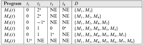
The results of executing Steps 3 through 9 are summarized in the following table. Column D indicates the contents of set D of distinguished mutants. As indicated, all mutants except M₂ are distinguished by T. Initially, all mutants are live.

As per Step 8 in Figure 8.1, execution of a mutant is interrupted soon after it has been distinguished. Entries marked NE in the table below indicate that the mutant in the corresponding row was not executed against the test case in the corresponding column. Note that mutant M₈ is distinguished by t₁ because its output is undefined (indicated by the entry marked “U”) due to division by 0. This implies that P(t₁) ≠ M₈(t₁). The first test case distinguishing a mutant is marked with an asterisk (*).

U: Output undefined. NE: Mutant not executed. ∗: First test to distinguish the mutant in the corresponding row.

 

Step 10: Live mutants

 

When none of the tests in Τ is able to distinguish mutant Μ from its parent Ρ, Μ is placed back into the set of live mutants. Of course, any mutant that is returned to the set of live mutants is not selected in Step 4 as it has already been selected once.

 

Example 8.13   In our example, there is only one mutant, M₂, that could not be distinguished by T_P. M₂ is returned to the set of live mutants in Step 10. Notice, however, that M₂ will not be selected again for classification as it has been selected once.

 

Step 11: Equivalent mutants

After having executed all mutants, one checks if there are any mutants remain live, i.e. set L is non-empty. Any remaining live mutants are tested for equivalence to their parent program. A mutant Μ is considered equivalent to its parent Ρ if for each test input from the input domain of P, the observed behavior of Μ is identical to that of P. We discuss the issue of determining whether or not a mutant is equivalent, in Section 8.7. The following example illustrates the process with respect to P8.1.

 

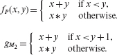
Example 8.14   Note from Example 8.13 that no test in T_P is able to distinguish M₂ from P and hence M₂ is live. We ask: is M₂ equivalent to P? An answer to such questions requires careful analysis of the behavior of the two programs: the parent and its mutant. In this case, let f_P(x, y) be the function computed by P and g_M2(x, y) that computed by M₂. The two functions follow.

 

To obtain an accurate mutation score for test Τ, one needs to determine which of the live mutants are equivalent to the parent program.

Rather than show that M₂ is equivalent to P, let us first attempt to find x = x₁ and y = y₁ such that f_P(x₁, y₁) ≠ g_M2 (x₁, y₁). A simple examination of the two functions reveals that the following two conditions, denoted as C₁ and C₂, must hold for f_P(x₁, y₁) ≠ g_M2 (x₁, y₁).

For the conjunct of C₁ and C₂ to hold, we must have x₁ = y₁ ≠ 0. We note that while test case t₁ satisfies C₁, it fails to satisfy C₂. However, the following test case does satisfy both C₁ and C₂.

 

t: < x = 1, y = 1 >

 

A simple computation reveals that P(t) = 1 and M₂(t) = 2. Thus we have shown that M₂ can be distinguished by at least one test case.

Hence, M₂ is not equivalent to its parent P. As there is only one live mutant in L that we have already examined for equivalence, we are done with Step 11. Set E of equivalent mutants remains empty.

 

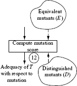
Step 12: Computation of mutation score

 

This is the final step in the assessment of test adequacy. Given sets L, D, and E, the mutation score, denoted by MS(T) of a test set Τ is computed as follows.

 

It is important to note that set L contains only the live mutants, none of which is equivalent to the parent. As is evident from the formula above, a mutation score is always between 0 and 1.

Given that |M| denotes the total number of mutants generated in Step 2, the following definition of mutation score is also used.

If a test set Τ distinguishes all mutants, except those that are equivalent, then |L| = 0 and the mutation score is 1. If T does not distinguish any mutant, then |D| = 0 and the mutation score is 0.

 

An interesting case arises when a test set does not distinguish any mutant and all mutants generated are equivalent to the original program. In this case, |D| = |L| = 0 and the mutant score is undefined. Hence we ask, Is the test set hopelessly inadequate ? The answer: No it is not. In this case, the set of mutants generated is insufficient to assess the adequacy of the test set. In practice, it is rare, if not impossible, to find a situation where |L| = |D| = 0 and all the generated mutants are equivalent to the parent. This fact will be evident when we discuss mutation operators in Section 8.4.

 

Note that a mutation score for a test set is computed with respect to a given set of mutants. Thus, there is no “golden” mutation score that remains fixed for a given test set. One will likely obtain different mutation scores for a test set evaluated against a different set of mutants. Thus, while a test set T might be perfectly adequate, i.e. MS(T) = 1 with respect to a given set of mutants, it might be perfectly inadequate, i.e. MS(T) = 0 with respect to another.

 

Example 8.15   Continuing with the illustrative example, it is easy to compute the mutation score for T_P as given in Example 8.7. At the start, there are eight mutants in Example 8.8. At the end of Step 11 there is one live mutant, seven distinguished mutants, and no equivalent mutant. Thus, |D| = 7, |L| = 1, and |E| = 0. This gives us MS(T_P) = 7/(7 + 1) = 0.875.

Test case t in Example 8.14 distinguishes the lone live mutant M₂ from its parent. Suppose t is added to T_P such that the test set so modified now contains five test cases. What is the revised mutation score for ? Obviously, However, T_P has been enhanced by adding t.

8.3.2  Alternate procedures for test adequacy assessment

Several variations of the procedure described in the previous section are possible, and often recommended. Let us start at Step 2. As indicated in Figure 8.1, Step 2 implies that all mutants are generated before test execution. However, an incremental approach might be better suited given the large number of mutants that will likely be created even for short programs, or for short functions within an application.

 

Using an incremental approach for the assessment of test adequacy, one generates mutants from only a subset of the mutation operators. The given test set is evaluated against this subset of mutants and a mutation score computed. If the score is less than 1, additional tests are created to ensure a score close to 1. This cycle is repeated with additional subsets of mutant operators and the test set further enhanced. The process may continue until all mutant operators have been considered.

The incremental approach allows an incremental enhancement of the test set at hand. This is in contrast to enhancing the test set at the end of the assessment process when a large number of mutants might remain live thereby overwhelming a tester.

It is also possible to use a multi-tester version of the process illustrated in Figure 8.1. Each tester can be assigned a subset of the mutation operators. The testers share a common test set. Each tester computes the adequacy with respect to the mutants generated by the operators assigned and enhances the test set. New tests so created are made available to the other testers through a common test repository. While this method of concurrent assessment of test adequacy might reduce the time to develop an adequate test set, it might lead to redundant tests (see Exercise 8.11).

8.3.3  “Distinguished” versus “killed” mutants

As mentioned earlier, a mutant that behaves differently than its parent program on some test input is considered killed. However, for the sake of promoting a sense of calm and peace during mutation testing, we prefer to use the term distinguished in lieu of killed. A cautionary note: most literature on mutation testing uses the term “killed.” Some people prefer to say that “a mutant has been detected” implying that the mutant referred to is distinguished from its parent.

 

Of course, a “distinguished mutant” is not distinguished in the sense of a “distinguished professor” or a “distinguished lady.” It is considered “distinguished from its parent by a test case.” Certainly, if a program mutant could feel and act like humans do, it probably will be happy to be considered “distinguished” like some of us do. Other possible terms for a distinguished mutant include extinguished and terminated.

8.3.4  Conditions for distinguishing a mutant

A test case t that distinguishes a mutant M from its parent P must satisfy the following three conditions labeled as C₁, C₂, and C₃.

1. C₁: Reachability: Must force the execution of a path from the start statement of Μ to the point of the mutated statement.
2. C₂: State infection: Must cause the state of M and P to differ consequent to some execution of the mutated statement.
3. C₃: State propagation: Must ensure that the difference in the states of M and P, created due to the execution of the mutated statement, propagates until after the end of mutant execution.

 

Thus a mutant is considered distinguished only when test t satisfies C₁ ^ C₂ ^ C₃. To be more precise, condition C₁ is necessary for C₂ which in turn is necessary for C₃. The following example illustrates the three conditions. Note that condition C₂ need not be true during the first execution of the mutated statement, though it must hold during some execution. Also, all program variables, and the location of program control, constitute program state at any instant during program execution.

A mutant is considered equivalent to the program under test if there is no test case in the input domain of P that satisfies each of the three conditions above. It is important to note that equivalence is based on identical behavior of the mutant and the program over the entire input domain and not just the test set whose adequacy is being assessed.

Example 8.16   Consider mutant M1 of Program P8.2. The reachability condition requires that control arrive at line 14. As this is a straight line program, with a return at the end, every test case will satisfy the reachability condition.

The state infection condition implies that after execution of the statement at line 14, the state of the mutant must differ from that of its parent. Let danger_P and danger_M denote the values of variable danger soon after the execution of line 14. The state infection condition is satisfied when danger_P ≠ danger_M. Any test case for which highcount = 3 satisfies the state infection condition.

Finally, as line 14 is the last statement in the mutant that can effect the state, no more changes can occur to the value of danger. Hence the state propagation condition is satisfied trivially by any test case that satisfies the state infection condition. Following is a test case that satisfies all three conditions.

 

t : < currentTemp = [20, 34, 29], maxTemp = 18 >

 

For test case t, we get P(t) = veryHigh and M(t) = none thereby distinguishing the mutant from its parent.

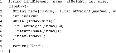
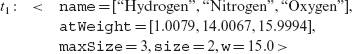
Example 8.17   Next consider function findElement, in P8.3, that searches for a chemical element whose atomic weight is greater than w. The function is required to return the name of the first such element found amongst the first size elements, or return “None” if no such element is found. Arrays name and atWeight contain, respectively, the element names and of the corresponding atomic weights. A global constant maxSize is the size the two arrays. Consider a mutant of P8.3 obtained by replacing the loop condition by index ≤ size.

Program P8.3

The reachability condition to distinguish this mutant is satisfied by any test case that causes findElement to be invoked. Let C_P and C_M denote, respectively, the loop conditions in P8.3 and its mutant. The state infection condition is satisfied by a test case for which the relation C_P ≠ C_M holds during some loop iteration.

The state propagation condition is satisfied when the value returned by the mutant differs from the one returned by its parent. The following test satisfies all three conditions.

Upon execution against t₁, the loop in P8.3 terminates unsuccessfully and the program returns the string “None.” On the contrary, when executing the mutant against t₁, the loop continues until index=size when it finds an element with atomic weight greater than w. While P8.3 returns the string “None,” the mutant returns “Oxygen.” Thus t₁ satisfies all three conditions for distinguishing the mutant from its parent. (Also see Exercises 8.8 and 8.10.)

8.4  Mutation Operators

In the previous sections, we gave examples of mutations obtained by making different kinds of changes to the program under test. Up until now, we have generated mutants in an ad hoc manner. However, there exists a systematic method, and a set of guidelines, for the generation of mutants that can be automated. One such systematic method and a set of guidelines are described in this section. We begin our discussion by learning what is a mutation operator and how is it used.

 

A mutation operator is a generative device. Other names used for mutation operators include mutagenic operator, mutant operator, and simply operator. In the remainder of this chapter, the terms “mutation operator” and “operator” are used interchangeably when there is no confusion.

Each mutation operator is assigned a unique name for ease of reference. For example, ABS and ROR are two names of mutation operators whose functions are explained in Example 8.18.

 

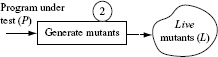
As shown in Figure 8.2, when applied to a syntactically correct program P, a mutation operator generates a set of syntactically correct mutants of P. We apply one or more mutation operators to P to generate a variety of mutants. A mutation operator might generate no mutants or one or more mutants. This is illustrated in the next example.

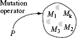
Figure 8.2 A set of k mutants M₁,M₂,...,M_kof P generated by applying a mutation operator. The number of mutants generated, k, depends on P and the mutation operator; k could be 0.

Example 8.18   Consider an operator named CCR. When applied to a program, CCR generates mutants by replacing each occurrence of a constant c by some other constant d; both c and d must appear in P. When applied to P8.1, CCR will not generate any mutant as the program does not contain any constant.

Next, consider an operator named ABS. When applied, ABS generates mutants by replacing each occurrence of an arithmetic expression e by the expression abs(e). Here it is assumed that abs denotes the “absolute value” function found in many programming languages. The following eight mutants are generated when ABS is applied to P8.1.

Location	Statement	Mutant
Line 4	if(x<y)	if(abs(x)<y)
		if(x<abs(y))
Line 5	output(x+y)	output(abs(x)+y)
		output(x+abs(y))
		output(abs(x+y))
Line 7	output(x*y)	output(abs(x)*y)
		output(x*abs(y))
		output(abs(x*y))

Note that the input statement and declarations have not been mutated. Declarations are not mutated and are considered the source for variables names and types to be used for certain types of mutations discussed later in this section. The input statement has not been mutated as adding an abs operator to an input value will lead to a syntactically incorrect program.

8.4.1  Operator types

Mutation operators are designed to model simple programming mistakes that programmers make. Faults in programs could be much more complex than the simple mistakes modeled by a mutation operator. However, it has been found that, despite the simplicity of mutations, complex faults are discovered while trying to distinguish mutants from their parent. We return to this suspicious sounding statement in Section 8.6.2.

 

It is to be noted that some mutation tools provide mutation operators designed explicitly to enforce code and domain coverage. The STRP is one such operator for languages C and Fortran. When applied to a program, it creates one mutant for each statement by replacing the statement with a trap condition. Such a mutant is considered distinguished from its parent when control arrives at the replaced statement. A test set that distinguishes all STRP mutants is considered adequate with respect to the statement coverage criterion.

The VDTR operator for C ensures that the given test set is adequate with respect to domain coverage for appropriate variables in the program under test. The domain is partitioned into a set of negative values, 0, and positive values. Thus, for an integer variable, domain coverage is obtained, and the corresponding mutants distinguished, by ensuring that the variables takes on any negative value, 0, and any positive value, during some execution of the program under test.

 

While a set of mutation operators is specific to a programming language, it can nevertheless be partitioned into a small set of generic categories. One such categorization appears in Table 8.1. While reading the examples in the table, read the right arrow (→) as mutates to. Also, note that in the first entry, constant 1 has been changed to 3, as constant 3 appears in another statement (y=y*3).

 

Table 8.1 A sample of generic categories of mutation operators and the common programming mistakes modeled.

Category	Mistake modeled	Examples
Constant mutation	Incorrect constant	x=x+1;→x=+3; y=y*3;→y=y*1;
Operator mutations	Incorrect operator	if(x<y)→if(x≤y) x++→++x
Statement mutation	Incorrectly placed statement	z=x+1;→delete
Variable mutations	Incorrectly used variable	z=x+1;→z=y+1; z=x+y;→z=abs(x)+y;

Only a set of four generic categories are shown in Table 8.1. As shown later in this section, in practice, there are many mutation operators under each category. The number and type of mutation operators under each category depend on the programming language for which the operators are designed.

The constant mutations category consists of operators that model mistakes made in the use of constants. Constants of different types, such as floats, integers, and booleans, are used in mutations. The domain of any mutation operator in this category is the set of constants appearing in the program that is mutated; a mutation operator does not invent constants. Thus, in the example that appears in Table 8.1, statement x=x+1 has been mutated to x=x+3 because constant 3 appears in another statement, i.e. in y=y*3.

The operator mutations category contains mutation operators that model common mistakes made in relation to the use of operators. Mistakes modeled include the incorrect use of arithmetic operators, relational operators, logical operators, and any other types of operators the language provides.

 

The statement mutation category consists of operators that model various mistakes made by programmers in the placement of statements in a program. These mistakes include incorrect placement of a statement, missing statement, incorrect loop termination, and incorrect loop formation.

The variable mutations category contains operators that model a common mistake programmers make when they incorrectly use a variable while formulating a logical or an arithmetic expression. Two incorrect uses are illustrated in Table 8.1. The first is the use of an incorrect variable x, a y should have been used instead. The second is an incorrect use of x, its absolute value should have been used. As with constant mutation operators, the domain of variable mutation operators includes all variables declared and used in the program being mutated. Mutation operators do not manufacture variables!

8.4.2  Language dependence of mutation operators

While it is possible to categorize mutation operators into a few generic categories, as in the previous section, the operators themselves are dependent on the syntax of the programming language. For example, for a program written in ANSI C (hereafter referred to as C), one needs to use mutation operators for C. A Java program is mutated using mutation operators designed for the Java language.

There are at least three reasons for the dependence of mutation operators on language syntax. First, given that the program being mutated is syntactically correct, a mutation operator must produce a mutant that is also syntactically correct. To do so requires that a valid syntactic construct be mapped to another valid syntactic construct in the same language.

 

Second, the domain of a mutation operator is determined by the syntax rules of a programming language. For example, in Java, the domain of a mutation operator that replaces one relational operator by another is {<, <=, >, >=, ! =, = =}.

Third, peculiarities of language syntax have an effect on the kind of mistakes that a programmer could make. Note that aspects of a language such as procedural versus object oriented, are captured in the language syntax.

Example 8.19   The Access Modifier Change (AMC) operator in Java replaces one access modifier, e.g. private, by another, e.g. public. This mutation models mistakes made by Java programmers in controlling the access of variables and methods.

While incorrect scoping is possible in C, the notion of access control is made explicit in Java though a variety of access modifiers and their combinations. Hence the AMC operator is justified for mutating Java programs. There is no matching operator for mutating C programs due to the absence of explicit access control; access control in C is implied by the location of declarations and can incorrect the placement of declarations often be checked by a compiler.

Example 8.20   Suppose x, y, and z are integer variables declared appropriately in a C program. The following is a valid C statement:

 

S: z=(x<y) ?0: 1;

 

Suppose now that we wish to mutate the relational operator in S. The relational operator < can be replaced by any one of the remaining five relational operators in C, namely = =, ! =, >, <=, and >=. Such a replacement would produce a valid statement in C, and in many other languages too given that the statement to be mutated is valid in that language.

However, C also allows the presence of any arithmetic operator in place of the < operator in the statement above. Hence, the < can also be replaced by any addition and multiplication operator from the set {+,–, *, /, %}. Thus, for example, while the replacement of < in S by the operator + will lead to a valid C statement, this would not be allowed in several other languages such as in Java and Fortran. This example illustrates that the domain of a mutation operator that mutates a relational operator is different in C than it is in Java.

This example also illustrates that the types of mistakes made by a programmer using C are different from those that a programmer might make, for instance, when using Java. It is perfectly legitimate to think that a C programmer has S as

 

S’: z=(x+y)? 0: 1;

 

for whatever reasons, whereas the intention was to code it as S. While both S and S' are syntactically correct, they might to different program behavior, only one of them being correct. It is easy to construct a large number of such examples of mutations, and mistakes, that a programmer might be able to make in one programming language but not in another.

The example above suggests that the design of mutation operators is a language dependent activity. Further, while it is possible to design mutation operators for a given programming language through guesses on what simple mistakes might a programmer make, a scientific approach is to base the design on empirical data. Such empirical data consolidates the common programming mistakes. In fact mutation operators for a variety of programming languages have been designed based on a mix of empirical evidence and collective programming experience of the design team.

8.5  Design of Mutation Operators

8.5.1  Goodness criteria for mutation operators

Mutation is a tool to assess the goodness of a test set for a given program. It does so with the help of a set of mutation operators that mutate the program under test into an often large number of mutants. Suppose that a test set T_P for program P is adequate with respect to a set of mutation operators M. What does this adequacy imply regarding the correctness of P ? This question leads us to the following definition.

Ideal set of mutation operators: Let Ρ_L denote the set of all programs in some language L. Let M_L be a set of mutation operators for L. M_L is considered ideal if (a) for any P ∈ Ρ, and any test set T_P against which Ρ is found to be correct with respect to its specification S, the adequacy of T_P with respect to M_L implies correctness of Ρ with respect to S and (b) there does not exist any M'_L smaller in size than M_L for which property (a) is satisfied.

 

Thus, an ideal set of mutant operators is minimal in size and ensures that adequacy with respect to this set implies correctness. While it is impossible to construct an ideal set of mutation operators for any but the most trivial of languages, it is possible to construct one that ensures correctness with relatively high probability. It is precisely such set of mutation operators that we desire. The implication of probabilistic correctness is best understood with respect to the “competent programmer hypothesis” and the “coupling effect” explained in Sections 8.6.1 and 8.6.2.

Properties (a) and (b), given in the definition of an ideal set of mutation operators, relate to the fault detection effectiveness and the cost of mutation testing. We seek a set of mutation operators that would force a tester into designing test cases that reveal as many faults as possible. Thus we desire high fault detection effectiveness. However, in addition, we would like to obtain high fault detection effectiveness at the lowest cost measured in terms of the number of mutants to be considered. The tasks of compiling, executing, and analyzing mutants are time consuming and must be minimized. The cost of mutation testing is generally lowered by a reduction in the number of mutants generated.

8.5.2  Guidelines

The guidelines here serve two purposes. One, they provide a basis on which to decide whether or not something should be mutated. Second, they help in understanding and critiquing an existing set of mutation operators such as the ones described later in this chapter.

It is to be noted that the design of mutation operators is as much of an art as it is science. Extensive experimentation, and experience with other mutation systems, is necessary to determine the goodness of a set of mutation operators for some language. However, to gain such experience, one needs to develop a set of mutation operators.

Empirical data on common mistakes serves as a basis for the design of mutation operators. In the early days of mutation research, mutation operators were designed based on empirical data available from various error studies. The effectiveness of these operators has been studied extensively. The guidelines provided here are based on past error studies, experience with mutation systems, and empirical studies to assess how effective are mutation operators in detecting complex errors in programs.

 

1. Syntactic correctness: A mutation operator must generate a syntactically correct program.
2. Representativeness: A mutation operator must model a common fault that is simple. Note that real faults in programs are often not simple. For example, a programmer might need to change significant portions of the code in order to correct a mistake that led to a fault. However, mutation operators are designed to model only simple faults, many of them taken together make up a complex fault.

   We emphasize that simple faults, e.g. a < operator mistyped as a > operator, could creep in due to a variety of reasons. However, there is no way to guarantee that for all applications, a simple fault will not lead to a disastrous consequence, e.g. a multimillion dollar rocket failure. Thus the term “simple fault” must not be equated with “simple,” “inconsequential,” or “low severity” failures.

3. Minimality and effectiveness: The set of mutation operators should be as small and effective as possible.
4. Precise definition: The domain and range of a mutation operator must be clearly specified; both depend on the programming language at hand. For example, a mutation operator to mutate a binary arithmetic operator, e.g. +, will have + in its domain as well in the range. However, in some languages, e.g. in C, replacement of a binary arithmetic operator by a logical operator, e.g. && will lead to a valid program. Thus all such syntax preserving replacements must be considered while defining the range.