8.6  Founding Principles of Mutation Testing

Mutation testing is a powerful testing technique for achieving correct, or close to correct, programs. It rests on two fundamental principles. One principle is commonly known as the competent programmer hypothesis (CPH), or the competent programmer assumption. The other is known as the coupling effect. We discuss these next.

 

8.6.1  The competent programmer hypothesis

The CPH arises from a simple observation made of practicing programmers. The hypothesis states that given a problem statement, a programmer writes a program Ρ that is in the general neighborhood of the set of correct programs.

An extreme interpretation of CPH is that when asked to write a program to find the account balance, given an account number, a programmer is unlikely to write a program that deposits money into an account. Of course, while such a situation is unlikely to arise, a devious programmer might certainly write such a program.

 

A more reasonable interpretation of the CPH is that the program written to satisfy a set of requirements will be a few mutants away from a correct program. Thus, while the first version of the program might be incorrect, it could be corrected by a series of simple mutations. One might argue against the CPH by claiming something like “What about a missing condition as the fault ? One would need to add the missing condition in order to arrive at a correct program.” Indeed, given a correct program P_c, one of its mutants is obtained by removing the condition from a conditional statement. Thus a missing condition does correspond to a simple mutant.

The CPH assumes that the programmer knows of an algorithm to solve the problem at hand, and if not, will find one prior to writing the program. It is thus safe to assume that when asked to write a program to sort a list of numbers, a competent program knows of, and makes use of, at least one sorting algorithm. Certainly, mistakes could be made while coding the algorithm. Such mistakes will lead to a program that can be corrected by applying one or more first order mutations.

8.6.2  The coupling effect

While the CPH arises out of observations of programmer behavior, the coupling effect is observed empirically. The coupling effect has been paraphrased by DeMillo, Lipton, and Sayward as follows.

 

Test data that distinguishes all programs differing from a correct one by only simple errors is so sensitive that it also implicitly distinguishes more complex errors.

Stated alternately, again in the words of DeMillo, Lipton, and Sayward “ . . . seemingly simple tests can be quite sensitive via the coupling effect.” As explained earlier, a “seemingly simple” first order mutant could be either equivalent to its parent or not. For some input, a non-equivalent mutant forces a slight perturbation in the state space of the program under test. This perturbation takes place at the point of mutation and has the potential of infecting the entire state of the program. It is during an analysis of the behavior of the mutant in relation to that of its parent that one discovers complex faults.

Extensive experimentation has revealed that a test set adequate with respect to a set of first order mutants, and is very close to being adequate with respect to second order mutants. Note that it may be easy to discover a fault that is a combination of many first order mutations. Almost any test will likely discover such a fault. It is the subtle faults that are close to first order mutations that are often difficult to detect. However, due to the coupling effect, a test set that distinguishes first order mutants is likely to cause an erroneous program under test to fail. This error detection aspect of mutation testing is explained in more detail in Section 8.8.

8.7  Equivalent Mutants

Given a mutant M of program P, we say that M is equivalent to P if P(t) = M(t) for all possible test inputs t. In other words, if Μ and Ρ behave identically on all possible inputs, then the two are equivalent.

The meaning of “behave identically” should be considered carefully. In strong mutation, the behavior of a mutant is compared with that of its parent at the end of their respective executions. Thus, for example, an equivalent mutant might follow a path different from that of its parent but the two might produce an identical output at termination.

A mutant that is equivalent under strong mutation might be distinguished from its parent under weak mutation. This is because in weak mutation the behavior of a mutant and its parent is generally compared at some intermediate point of execution.

The general problem of determining whether or not a mutant is equivalent to its parent is undecidable and equivalent to the halting problem. Hence, in most practical situations, determination of equivalent mutants is done by the tester through careful analysis. Some methods for the automated detection of equivalent mutants are pointed under bibliographic notes.

 

It should be noted that the problem of deciding the equivalence of a mutant in mutation testing is analogous to that of deciding whether or a given path is infeasible in, say, MC/DC or data flow testing. Hence, it is unwise to consider the problem of isolating equivalent mutants from non-equivalent ones as something that makes mutation testing less attractive than any other form of coverage-based assessment of test adequacy.

8.8  Fault Detection Using Mutation

Mutation offers a quantitative criterion to assess the adequacy of a test set. A test set T_P for program P, inadequate with respect to a set of mutants, offers an opportunity to construct new tests that will hopefully exercise Ρ in ways different from those it has already been exercised. This in turn raises the possibility of detecting hidden faults that so far have remained undetected despite the execution of Ρ against T_P. In this section, we show how mutants force the construction of new tests that reveal faults not necessarily modeled directly by the mutation operators.

 

We begin with an illustrative example that shows how a missing condition fault is detected in an attempt to distinguish a mutant created using a mutation operator analogous to the VLSR operator in C.

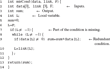
Example 8.21   Consider a function named misCond. It takes zero or more sequence of integers in array data as input. It is required to sum all integers in the sequence starting from the first integer and terminating at the first 0. Thus, for example, if the input sequence is (6 5 0), then the program must output 11. For the sequence (6 5 0 4), misCond must also output 11.

Array link specifies the starting location of each sequence in data. Array subscripts are assumed to begin at 0. An integer F points to the first element of a sequence in data to be summed. link(F) points to the second element of this sequence, link(link(F)) to the third element, and so on. A – 1 in a link entry implies the end of a sequence that begins at data(F).

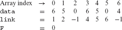
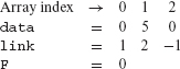
Sample input data is shown below, data contains the two sequences (6 5 0) and (6 5 0 4). F is 0 indicating that the function needs to sum the sequence starting at data(F) which is (6 5 0). Setting F to 3 specifies the second of the two sequences in data.

In the sample inputs shown above, the sequence is stored in contiguous locations in data. However, this is not necessary and link can be used to specify an arbitrary storage pattern.

Function misCond has a missing condition error. The condition at line 7 should be

 

((L ≠ – l) and (data[L] ≠0)).

 

Let us consider a mutant Μ of misCond created by mutating line 9 to the following:

 

if(data[F] ≠0) sum = sum + data[L];

 

We will show that Μ is an error-revealing mutant. Notice that variable L has been replaced by F. This is a typical mutant generated by several mutation testing tools when mutating with the variable replacement operator, e.g. the VLSR operator in C.

 

A mutant Μ is considered “error-revealing” when a test that distinguishes Μ also reveals an error in its parent program.

We will now determine a test case that distinguishes Μ from misCond. Let C_P and C_M denote the two conditions data(L) ≠ 0 and data(F) ≠ 0, respectively. Let SUM_P and SUM_M denote, respectively, the values of SUM when control reaches the end of misCond and M. Any test case t that distinguishes Μ must satisfy the following conditions:

1. Reachability: There must be a path from the start of misCond to the mutated statement at line 9.
2. State infection: C_P ≠ C_M must hold at least once through the loop.
3. State propagation: SUM_P ≠ SUM_M.

We must have L = F ≠ – 1 for the reachability condition to hold. During the first iteration of the loop we have F=L due to the initialization statement immediately preceding the start of the loop. This initialization forces C_P = C_M during the first iteration. Therefore, the loop must be traversed at least twice implying that link(F) ≠ – 1. Any one of the following two conditions could be true during the second or subsequent loop traversals.

However, (8.1) will not guarantee state propagation because adding 0 to SUM will not alter its value from the previous iteration. Condition (8.2) will guarantee state propagation but only if the sum of the second and any subsequent elements of the sequence being considered is non-zero.

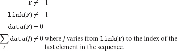
In summary, a test case t must satisfy the following conditions for misCond(t) ≠ M(t):

Suppose P_c denotes the correct version of misCond. It is easy to check that for any t that satisfies the four conditions above, we get P_c(t) = 0, whereas the incorrect function misCond (t) ≠ 0. Hence test case t causes misCond to fail thereby revealing the existence of a fault. A sample error-revealing test case follows.

Exercises 8.19 and 8.20 provide additional examples of error revealing mutants. Exercise 8.21 is designed to illustrate the strength of mutation with respect to path oriented adequacy criteria.

In the above example, we have shown that an attempt to distinguish the variable replacement operator forces the construction of a test case that causes the program under test to fail. We now ask: Are there other mutations of misCond that might reveal the fault ? In general, such questions are difficult, if not impossible, to answer without the aid of a tool that automates the mutant generation process. Next we formalize the notion of an error revealing mutant such as the one we have seen in the previous example.

8.9  Types of Mutants

We now provide a formalization of the error detection process exemplified above. Let Ρ denote the program under test that must conform to specification S. D denotes the input domain of Ρ derived from S. Each mutant of Ρ has the potential of revealing one or more possible errors in P. However, for one reason or another it may not reveal any error. From a tester’s point of view, we classify a mutant into one of three types: error revealing, error hinting, and reliability indicating. Let P_c denote a correct version of P. Consider the following three types of mutants.

 

A mutant Μ is said to be of type error revealing (ε) for program Ρ if and only if ∀t∈D such that P(t) ≠ M(t), P(t) ≠ P_c(t) and that there exists at least one such test case, t is considered to be an error revealing test case.

A mutant Μ is said to be of type error hinting (H), if and only if Ρ ≡ Μ and P_c ≢ Μ.

A mutant Μ is said to be ot type reliability indicating (R) it and only it P(t) ≠ M(t) for some t ∈ D and P_c(t) = P(t).

 

Let S_x denote the set of all mutants of type x. From the definition of equivalence, we have S_ε ∩ S_H =∅ and S_H ∩ S_R =∅. A test case that distinguishes a mutant either reveals the error in which case it belongs to S_ε, or else it does not reveal the error in which case it belongs to S_R. Thus S_ε ∩ S_R = ∅.

During testing a tool such as MuJava or Proteum generates mutants of Ρ and executes them against all tests in Τ. It is during this process that one determines the category to which a mutant belongs. There is no easy, or automated way, to find which of the generated mutants belongs to which of the three classes mentioned above. However, experiments have revealed that if there is an error in P, then with high probability at least one of the mutants is error revealing.

8.10  Mutation Operators for C

In this section, we take a detailed look at the mutation operators designed for the C programming language. As mentioned earlier, the entire set of 77 mutation operators is divided into four categories: constant mutations, operator mutations, statement mutations, and variable mutations. The contents of this section should be particularly useful to those undertaking the task of designing mutation operators and developing tools for mutation testing.

 

The set of mutation operators introduced in this section was designed at Purdue University by a group of researchers led by Richard A. Demillo. This set is perhaps the largest, most comprehensive, and the only set of of mutation operators known for C. Josè Maldonado’s research group at the University of Saõ Carlos at Saõ Carlos, Brazil, has implemented the complete set of C mutation operators in a tool named Proteum. In Section 8.12, we compare the set of mutation operators with those for some other languages. Section 8.15 points to some tools to assist a tester in mutation testing.

8.10.1  What is not mutated ?

Every mutation operator has a possibly infinite domain on which it operates. The domain itself consists of instances of syntactic entities, which appear within the program under test, mutated by the operator. For example, the mutation operator that replaces a while statement by a do-while statement has all instances of the while statements in its domain. This example, however, illustrates a situation in which the domain is known.

 

Consider a C function having only one declaration statement int x, y, z. What kind of syntactic aberrations can one expect in this declaration? One aberration could be that though the programmer intended z to be a real variable, it was declared as an integer. Certainly, a mutation operator can be defined to model such an error. However, the list of such aberrations is possibly infinite and, if not impossible, difficult to enumerate. The primary source of this difficulty is the infinite set of type and identifier associations to select from. Thus it becomes difficult to determine the domain for any mutant operator that might operate on a declaration.

The above reasoning leads us to treat declarations as universe defining entities in a program. The universe defined by a declaration, such as the one mentioned above, is treated as a collection of facts. Declaration int x, y, z states three facts, one for each of the three identifiers. Once we regard declarations to be program entities that state facts, we cannot mutate them because we have assumed that there is no scope for any syntactic aberration. With this reasoning as the basis, declarations in a C program are not mutated. Errors in declarations are expected to manifest through one or more mutants.

Following is the complete list of entities that are not mutated.

• Declarations
• The address operator (&)
• Format strings in input-output functions
• Function declaration headers
• Control line
• Function name indicating a function call. Note that actual parameters in a call are mutated, but the function name is not. This implies that I/O function names such as scanf, printf, open, and so on are not mutated
• Preprocessor conditionals

8.10.2  Linearization

In C, the definition of a statement is recursive. For the purpose of understanding various mutation operators in the statement mutations category, we introduce the concept of linearization and reduced linearized sequence.

Let S denote a syntactic construct that can be parsed as a C statement. Note that statement is a syntactic category in C. For an iterative or selection statement denoted by S, ^cS denotes the condition controlling the execution of S. If S is a for statement, then ^eS denotes the expression executed immediately after one execution of the loop body and immediately before the next iteration of the loop body, if any, is about to begin. Again, if S is a for statement, then ⁱS denotes the initialization expression executed exactly once for each execution of S. If the controlling condition is missing, then ^cS defaults to true.

Using the above notation, if S is an if statement, we shall refer to the execution of S in an execution sequence as ^cS. If S denotes a for statement, then in an execution sequence we shall refer to the execution of S by one reference to ⁱS, one or more references to ^cS, and zero or more references to ^eS. If S is a compound statement, then referring to S in an execution sequence merely refers to any storage allocation activity.

Example 8.22   Consider the following for statement:

 

for (m=0, n=0; isdigit(s[i]); i++)

    n = 10* n + (s[i]) - ’0’);

 

Denoting the above for statement by S, we get,

 

ⁱS: m=0, n=0

^cS: isdigit(s[i]), and

^eS: i++.

 

If S denotes the following for statement,

then we have,

 

ⁱS:; (the null expression-statement),

^cS: true, and

^eS:; (the null expression-statement).

 

Let T_f and T_s denote, respectively, the parse trees of function f and statement S. A node of T_s is said to be identifiable if it is labeled by any one of the following syntactic categories:

• statement
• labeled statement
• expression statement
• compound statement
• selection statement
• iteration statement
• jump statement

A linearization of S is obtained by traversing T_s in preorder and listing, in sequence, only the identifiable nodes of T_s.

 

For any X, let denote the sequence X_j X_j+1 . . . X_i−1 X_i. Let denote the linearization of S. If S_i S_i+1 is a pair of adjacent elements in S_L such that S_i+1 is the direct descendent of S_i in T_S and there is no other direct descendent of S_i then S_iS_i+1 is considered to be a collapsible pair with S_i being the head of the pair. A reduced linearized sequence of S, abbreviated as RLS, is obtained by recursively replacing all collapsible elements of S_L by their heads. The RLS of a function is obtained by considering the entire body of the function as S and finding the RLS of S. The RLS, obtained by the above method, will yield a statement sequence in which the indices of the statements are not increasing in steps of 1. We shall always simplify the RLS by renumbering its elements, so that for any two adjacent elements S_iS_j, we have j = i+1.

We shall refer to the RLS of a function f and a statement S by RLS(f) and RLS(S), respectively.

8.10.3  Execution sequence

Though most mutation operators are designed to simulate simple faults, the expectation of mutation-based testing is that such operators will eventually reveal one or more errors in the program. In this section, we provide some basic definitions that are useful in understanding such operators and their dynamic effects on the program under test.

When f executes, the elements of RLS(f) will be executed in an order determined by the test case and any path conditions in RLS(f). Let be the execution sequence of for test case t, where S_j, 1 ≤ j ≤ m − 1 is any one of S_i, 1 ≤ i ≤ n and S_i is not a return statement. We assume that f terminates on t. Thus S_m = R^', where R' is R or any other return statement in RLS(f).

Any proper prefix of E(f, t), where S_k = R', is a prematurely terminating execution sequence (subsequently referred to as PTES for brevity) and is denoted by E^p(f, t). is known as the suffix of E(f, t) and is denoted by E^s(f, t); E^s(f, t); E^l(f, t) denotes the last statement of the execution sequence of f. If f is terminating, E^l(f, t)=return.

Let and be two execution sequences. We say that E₁ and E₂ are identical if and only if i = k, j = l, and S_q = Q_q, i ≤ q ≤ j. As a simple example, if f and f' consist of one assignment each, namely, a = b + c and a = b – c, respectively, then there is no t for which E(f, t) and E(f', t) are identical. It must be noted that the output generated by two execution sequences may be the same even though the sequences are not identical. In the above example, for any test case t that has c = 0, P_f(t) = P_f'(t).

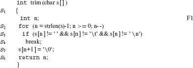
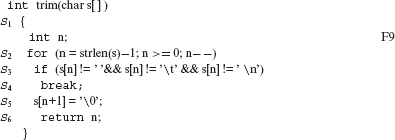
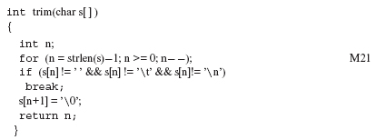
Example 8.23   Consider the function trim defined below. Note that this and several other illustrative examples in this chapter borrow program fragments for mutation from the well-known book by Brian Kernighan and Dennis Ritchie titled “The C programming Language.”

/* This function is from p 65 of Kernighan and Ritchie’s book. */

We have RLS(trim) = S₁ S₂ S₃ S₄ S₅ S₆. Let the test case t be such that the input parameter s evaluates to ab (a space character follows b), then the execution sequence E(trim, t) is: S₁ ⁱS₂ ^cS₂ ^cS₃ ^cS₂ ^cS₃ S₄ S₅ S₆. S₁ ⁱS₂ is one prefix of E(f, t) and S₄ S₅ S₆ is one suffix of E(trim, t). Note that there are several other prefixes and suffixes of E(trim, t). S₁ ⁱS₂ ^cS₂ S₆ is a proper prefix of E(f, t).

 

The reduced linearized sequence of a statement aids in determining the domain of mutation operators that have statements in their domain.

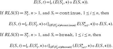
Analogous to the execution sequence for RLS(f), we define the execution sequence of RLS(S) denoted by E(S, t) with E^p(S, t), E^S(S, t), and E^l(S, t) corresponding to the usual interpretation.

The composition of two execution sequences and is written as E₁ ο E₂. The conditional composition of E₁ and E₂ with respect to condition c is written as E₁ |_c E₂. It is defined as:

In the above definition, condition c is assumed to be evaluated after the entire E₁ has been executed. Note that ο has the same effect as |_true. ο associates from left to right and |_c associates from right to left. Thus, we have:

E(f, *) (E(S, *)) denotes the execution sequence of function f (statement S) on the current values of all the variables used by f (S). We shall use this notation while defining execution sequences of C functions and statements.

Let S, S₁, and S₂ denote a C statement other than break, continue, goto, and switch, unless specified otherwise. The following rules can be used to determine execution sequences for any C function.

 

R 1 E({ },t) is the null sequence.

R 2 E({ }, t) ο E(S, t) = E(S, t) = E(S, t) ο E({ })

R 3

R 4 If S is an assignment-expression, then E(S, t) = S.

R 5 For any statement S, E(S, t) = RLS(S), if RLS(S) contains no statements other than zero or more assignment-expressions. If RLS(S) contains any statement other than the assignment-expression, the above equality is not guaranteed due to the possible presence of conditional and iterative statements.

R 6 If S = S₁; S₂; then E(S, t) = E(S₁, t) ο E(S₂, ∗).

R 7 If S = while (c) S'₁ , then

R 8 If S = do S₁while(c); then

 

 

If RLS(S) contains a continue, or a break, then its execution sequence can be derived using the method indicated for the while statement.

R 9 If S = if (c) S₁, then

 

 

R 10 If S = if (c) S₁ else: S₂, then

Example 8.24   Consider S₃, the if statement, in F1. We have RLS(S₃) = S₃ S₄. Assuming the test case of the Example 8.23 and n = 3, we get E(S₃, *) = ^cS₃. If n = 2, then E(S₃, *) = ^cS₃ S₄. Similarly, for S₂, which is a for statement, we get E(S₂,*) = ⁱS₂ ^cS₂ ^cS₃ ^cS₂ ^cS₃ S₄. For the entire function body, we get E(trim, t) = S₁ E(S₂, *) ο E(S₅, *) ο E(S₆, *).

8.10.4  Effect of an execution sequence

As before, let P denote the program under test, f a function in P, that is to be mutated, and t a test case. Assuming that P terminates, let P_f (t) denote the output generated by executing P on t. The subscript f with P is to emphasize the fact that it is the function f that is being mutated.

 

We say that E(f, *) has a distinguishable effect on the output of P, if P_f (t) ≠ P_f' (t), where f' is a mutant of f. We consider E(f, *) to be a distinguishing execution sequence (DES) of P_f(t) with respect to f'.

Given f and its mutant f', for a test case t to distinguish f', it is necessary, but not sufficient, that E(f, t) be different from E(f', t). The sufficiency condition is that P_f(t) ≠ P_f'(t) implying that E(f, t) is a DES for P_f(t) with respect to f'.

While describing the mutant operators, we shall often use DES to indicate when a test case is sufficient to distinguish between a program and its mutant. Examining the execution sequences of a function, or a statement, can be useful in constructing a test case that distinguishes a mutant.

Example 8.25   To illustrate the notion of the effect of an execution sequence, consider the function trim defined in F1. Suppose that the output of interest is the string denoted by s. If the test case t is such that s consists of the three characters a, b, and space, in that order, then E(trim, t) generates the string ab as the output. As this is the intended output, we consider it to be correct.

Now suppose that we modify trim by mutating S₄ in F1 to continue. Denoting the modified function by trim', we get

 

E(trim', t) = S₁ ⁱS₂ ^cS₂ ^cS₃ ^eS₂ ^cS₃ ^eS₂ ^cS₃ S₄ ^eS₂ ^cS₃ S₄ ^eS₂ S₅ S₆).

 

The output generated due to E(trim', t) is different from that generated due to E(trim, t). Thus, E(trim, t) is a DES for P_trim(t) with respect to the function trim'.

DESs are essential to kill mutants. To obtain a DES for function f, a suitable test case t needs to be constructed such that E(f, t) is a DES for P_f(t) with respect to f'.

8.10.5  Global and local identifier sets

For defining variable mutations in Section 8.10.10, we need the concept of global and local sets, defined in this section, and global and local reference sets, defined in the next section.

 

Let f denote a C function to be mutated. An identifier denoting a variable, that can be used inside f, but is not declared in f, is considered global to f. Let G_f denote the set of all such global identifiers for f. Note that any external identifier is in G_f unless it is also declared in f. While computing G_f , it is assumed that all files specified in one or more # include control lines have been included by the C preprocessor. Thus any global declaration within the files listed in a # include also contributes to G_f .

Let L_f denote the set of all identifiers declared either as parameters of f or at the head of its body. Identifiers denoting functions do not belong to G_f or L_f .

In C, it is possible for a function f to have nested compound statements such that an inner compound statement S has declarations at its head. In such a situation, the global and local sets for S can be computed using the scope rules in C.

We define GS_f , GP_f , GT_f , and GA_f as subsets of G_f which consist of, respectively, identifiers declared as scalars, pointers to an entity, structures, and arrays. Note that these four subsets are pairwise disjoint. Similarly, we define LS_f , LP_f , LT_f , and LA_f as the pairwise disjoint subsets of L_f .

8.10.6  Global and local reference sets

Use of an identifier within an expression is considered a reference. In general, a reference can be multilevel implying that it can be composed of one or more subreferences. Thus, for example, if ps is a pointer to a structure with components a and b, then in (*ps).a, ps is a reference and *ps and (*ps).a are two subreferences. Further, *ps.a is a 3-level reference. At level 1, we have ps, at level 2 we have (*ps), and finally at level 3 we have (*ps).a. Note that in C, (*ps).a has the same meaning as ps–>a.

 

The global and local reference sets consist of references at level 2 or higher. Any references at level 1 are in the global and local sets defined earlier. We shall use GR_f and LR_f to denote, respectively, the global and local reference sets for function f.

Referencing a component of an array or a structure may yield a scalar quantity. Similarly, dereferencing a pointer may also yield a scalar quantity. All such references are known as scalar references. Let GRS_f and LRS_f denote sets of all such global and local scalar references, respectively. If a reference is constructed from an element declared in the global scope of f, then it is a global reference, otherwise it is a local reference.

We now define GS'_f and LS'_f by augmenting GS_f and LS_f as follows:

GS'_f and LS'_f are termed as scalar global and local reference sets for function f, respectively.

Similarly, we define array, pointer, and structure reference sets denoted by GRA_f , GRP_f , GRT_f , LRA_f , LRP_f , and LRT_f . Using these, we can construct the augmented global and local sets GA'_f , GP'_f , GT'_f , LA'_f , LP'_f , and LT'_f .

For example, if an array is a member of a structure, then a reference to this member is an array reference and hence belongs to the array reference set. Similarly, if a structure is an element of an array, then a reference to an element of this array is a structure reference and hence belongs to the structure reference set.

On an initial examination, our definition of global and local reference sets might appear to be ambiguous especially with respect to a pointer to an entity. An entity in the present context can be a scalar, an array, a structure, or a pointer. Function references are not mutated. However, if fp is a pointer to some entity, then fp is in set GRP_f or LRP_f depending on its place of declaration. On the other hand, if fp is an entity of pointer(s), then it is in any one of the sets GRX_f or LRX_f where X could be any one of the letters A, P, or T.

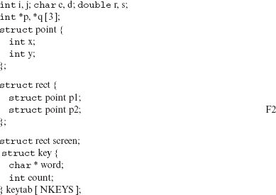
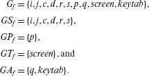
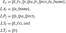
Example 8.26   To illustrate our definitions, consider the following external declarations for function f.

The global sets corresponding to the above declarations are

Note that structure components x, y, word, and count do not belong to any global set. Type names, such as rect and key above, are not in any global set. Further, type names do not participate in mutation due to reasons outlined in Section 8.10.1.

Now, suppose that the following declarations are within function f .

 

int fi; double fx; int *fp; int (*fpa) (20)

struct rect fr; struct rect *fprct;

int fa [10]; char *fname [nchar]

 

Then the local sets for f are

To illustrate reference sets, suppose that f contains the following references (the specific statement context in which these references are made is of no concern for the moment).

 

i * j + fi

r + s – fx + fa[ i ]

*p + = 1

*q [j ] = *p

screen . p1 = screen . p2

screen . p1 . x = i

keytab [j ] . count = *p

p = q[i ]

fr = screen

*fname [j ] = keytab [ i ] .word

fprct = & screen

 

The global and local reference sets corresponding to the above references are

The above sets can be used to augment the local sets.

Analogous to the global and local sets of variables, we define global and local sets of constants: GC_f and LC_f . GC_f is the set of all constants global to f. LC_f is the set of all constants local to f. Note that a constant can be used within a declaration or in an expression.

We define GCI_f , GCR_f , GCC_f , and GCP_f to be subsets of GC_f consisting of only integer, real, character, and pointer constants. GCP_f consists of only null. LCI_f , LCR_f , LCC_f , and LCP_f are defined similarly.

8.10.7  Mutating program constants

We begin our introduction to the mutation operators for C with operators that mutate constants. These operators model coincidental correctness and, in this sense, are similar to scalar variable replacement operators discussed later in Section 8.10.10. A complete list of such operators is available in Table 8.2.

 

Table 8.2 Mutation operators for the C programming language that mutate program constants.

Mutop	Domain	Description
CGCR	Constants	Constant replacement using global constants
CLSR	Constants	Constant for scalar replacement using local constants
CGSR	Constants	Constant for scalar replacement using global constants
CRCR	Constants	Required constant replacement
CLCR	Constants	Constant replacement using local constants

Required constant replacement

 

Let I and R denote, respectively, the sets {0, 1, –1, u_i} and {0.0, 1.0, –1.0, u_r}. u_i and u_r denote user specified integer and real constants, respectively. Use of a variable, where an element of I or R was the correct choice, is the fault modeled by CRCR.

Each scalar reference is replaced systematically by elements of I or R. If the scalar reference is integral, I is used. For references that are of type floating, R is used. Reference to an entity via a pointer is replaced by null. Left operands of the assignment operators as well as the ++ and – – operators are not mutated.

 

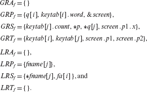
Example 8.27   Consider the statement k=j+ *p, where k and j are integers and p is a pointer to an integer. When applied to the above statement, the CRCR mutation operator generates the following mutants.

A CRCR mutant encourages a tester to design at least one test case that forces the variable replaced to take on values other than from the set I or R. Thus such a mutant attempts to overcome coincidental correctness of P.

 

Constant for Constant Replacement

 

Just as a programmer may mistakenly use one identifier for another, a possibility exists that one may use a constant for another. Mutation operators CGCR and CLCR model such faults. These two operators mutate constants in f using, respectively, the sets GC_f and LC_f .

Example 8.28   Suppose that constant 5 appears in an expression, and GC_f = {0,1.99,' c'}, then 5 will be mutated to 0, 1.99, and 'c' thereby producing three mutants. 

Pointer constant, null, is not mutated. Left operands of assignment, ++ and – – operators are also not mutated.

 

Constant for Scalar Replacement

 

Use of a scalar variable, instead of a constant, is the fault modeled by mutation operators CGSR and CLSR. CGSR mutates all occurrences of scalar variables or scalar references by constants from the set GC_f . CLSR is similar to CGSR except that it uses LC_f for mutation. Left operands of assignment, ++ and – – operators are not mutated.

 

8.10.8  Mutating operators

Mutation operators in this category model common errors made while using various operators in C. Do not be confused with the overloaded use of the term “operator.” We use the term “mutation operator” to refer to a mutation operator as discussed earlier, and the term “operator” to refer to the operators in C such as the arithmetic operator + or the relational operator <.

8.10.9  Binary operator mutations

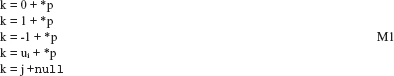
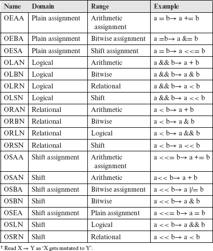
The incorrect choice of a binary C-operator within an expression is the fault modeled by this mutation operator. The binary mutation operators fall into two categories: Comparable Operator Replacement (Ocor) and Incomparable Operator Replacement (Oior). Within each subcategory, the mutation operators correspond to either the non-assignment or to the assignment operators in C. Tables 8.3, 8.4, and 8.5 list all binary mutation operators in C.

 

Each binary mutation operator systematically replaces a C operator in its domain by operators in its range. The domain and range for all mutation operators in this category are specified in Tables 8.3, 8.4, and 8.5. In certain contexts, only a subset of arithmetic operators is used. For example, it is illegal to add two pointers, though a pointer may be subtracted from another. All mutation operators that mutate C-operators, are assumed to recognize such exceptional cases to retain the syntactic validity of the mutant.

 

Table 8.3 Domain and range of mutation operators in Ocor.

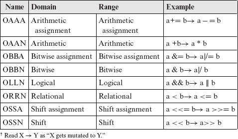
Table 8.4 Domain and range of mutation operators in Oior: arithmetic and bitwise.

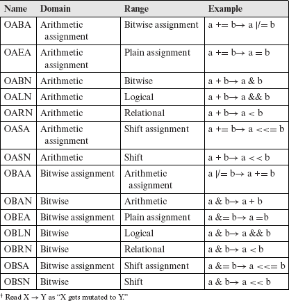
Table 8.5 Domain and Range of mutation operators in Oior: plain, logical, and relational.

Unary operator mutations

 

Mutations in this subcategory consist of mutation operators that model faults in the use of unary operators and conditions. Operators in this category fall into the five subcategories described in the following.

 

Increment/Decrement: The ++ and – – operators are used frequently in C programs. The ΟΡΡΟ and OMMO mutation operators model the faults that arise from the incorrect use of these C operators. The incorrect uses modeled are: (a) ++ (or – –) used instead of – – (or ++) and (b) prefix increment (decrement) used instead of postfix increment (decrement).

The ΟΡΡΟ operator generates two mutants. An expression such as ++x is mutated to x++ and – –x. An expression, such as x++, will be mutated to ++x and x– –. The OMMO operator behaves similarly. It mutates – –x to x– – and ++x. It also mutates x– – to – –x and x++. Both the operators will not mutate an expression if its value is not used. For example, an expression such as i++ in a for header will not be mutated, thereby avoiding the creation of an equivalent mutant. An expression such as *x++ will be mutated to *++x and *x– –.

Logical Negation: Often, the sense of the condition used in iterative and selective statements is reversed. OLNG models this fault. Consider the expression x op y, where op can be any one of the two logical operators: && and ||. OLNG will generate three mutants of such an expression as follows: x op !y, !x op y, and !(x op y).

Logical Context Negation: In selective and iterative statements, excluding the switch, often the sense of the controlling condition is reversed. OCNG models this fault. The controlling condition in the iterative and selection statements is negated. The following examples illustrate how OCNG mutates expressions in iterative and selective statements.

 

if (expression) statement →

    if (! expression) statement

 

if (expression) statement else statement →

    if (! expression) statement else statement

 

while (expression) statement →

    while (! expression) statement

 

do statement while (expression) →

    do statement while (! expression)

 

for (expression; expression; expression) statement →

    for (expression; ! expression, expression)statement

 

expression ? expression : conditional expression →

    !expression ? expression : conditional expression

 

When applied on an iteration statement, application of the OCNG operator may generate mutants with infinite loops. Further, this application may also generate mutants generated by OLNG. Note that a condition such as (x<y) in an if statement will not be mutated by OLNG. However, the condition ((x<y&&p>q) will be mutated by both OLNG and OCNG to (!(x<y)&&(p>q)).

Bitwise Negation: The sense of the bitwise expressions may often be reversed. Thus, instead of using (or not using) the one’s complement operator, the programmer may not use (or may use) the bitwise negation operator. The OBNG operator models this fault.

Consider an expression of the form x op y, where op is one of the bitwise operators: |/ and &. The OBNG operator mutates this expression to: x op~ y,~ x op y, and ~(x op y). OBNG does not consider the iterative and conditional operators as special cases. Thus, for example, a statement such as if (x && a |/ b) p = q will get mutated to the following statements by OBNG:

 

if (x && a |/~ b)p = q

if (x &&~ a |/b)p = q

if (x &&~ (a |/b))p = q

 

Indirection Operator Precedence Mutation: Expressions constructed using a combination of ++, – –, and the indirection operator (*), can often contain precedence faults. For example, using *p++ when (*p)++ was meant, is one such fault. OIPM operator models such faults.

OIPM mutates a reference of the form * x op to (*x) op and op (*x), where op can be ++ and – –. Recall that in C, * x op implies * (x op). If op is of the form [y], then only (*x) op is generated. For example, a reference such as *x[p] will be mutated to (*x)[p].

The above definition is for the case when only one indirection operator has been used to form the reference. In general, there could be several indirection operators used in formulating a reference. For example, if x is declared as int ***x, then ***x++ is a valid reference in C. A more general definition of OIPM takes care of this case.

Consider the following reference x op. OIPM systematically mutates this reference to the following references:

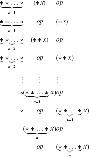
Multiple indirection operators are used infrequently. Hence, in most cases, we expect OIPM to generate two mutants for each reference involving the indirection operator.

Cast Operator Replacement: A cast operator, referred to as cast, is used to explicitly indicate the type of an operand. Faults in such usage are modeled by OCOR.

Every occurrence of a cast operator is mutated by OCOR. Casts are mutated in accordance with the restrictions listed below. These restrictions are derived from the rules of C as specified in the ANSI C standard. While reading the cast mutations described below, ↔ may be read as “gets mutated to.” All entities to the left of ↔ get mutated to the entities on its right and vice versa. The notation X* can be read as “X and all mutations of X excluding duplicates.”

 

char ↔ signed char unsigned char

int* float*

 

int ↔ signed int unsigned int

short int long int

signed long int signed long int

float* char*

 

float ↔ double long double

int* char*

 

double ↔ char* int*

float*

Example 8.29   Consider the statement:

return (unsigned int) (next/65536) % 32768

 

Sample mutants generated when OCOR is applied to the above statement are shown below (only cast mutations are listed).

 

short int long int

float double

 

Note that the cast operators, other than those described in this section, are not mutated. For example, the casts in the following statement are not mutated:

 

 

The decision not to mutate certain casts was motivated by their infrequent use and the low probability of a fault that could be modeled by mutation. For example, a cast such as void ** is used infrequently and when used, the chances of it being mistaken for, say, an int, appear to be low.

8.10.10  Mutating statements

We now describe each one of the mutation operators that mutate entire statements or their key syntactic elements. A complete list of such operators is given in Table 8.6. For each mutation operator, its definition and the fault modeled is provided. The domain of a mutation operator is described in terms of the effected syntactic entity.

 

Table 8.6 List of mutation operators for statements in C.

Mutop	Domain	Description
SBRC	break	break replacement by continue
SBRn	break	Break out to nth level
SCRB	continue	continue replacement by break
SDWD SGLR	do-while goto	do-while replacement by while goto label replacement
SMVB	Statement	Move brace up and down
SRSR	return	return replacement
SSDL	Statement	Statement deletion
SSOM	Statement	Sequence Operator Mutation
STRI	if Statement	Trap on if condition
STRP	Statement	Trap on statement execution
SMTC	Iterative statements	n-trip continue
SSWM	switch statement	switch statement mutation
SMTT	Iterative statement	n–trip trap
SWDD	while	while replacement by do-while

Recall that some statement mutation operators are included to ensure code coverage and do not model any specific fault. The STRP is one such operator.

The operator and variable mutations described in subsequent sections, also effect statements. However, they are not intended to model faults in the explicit composition of the selection, iteration, and jump statements.

Trap on Statement Execution

 

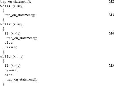
This operator is intended to reveal unreachable code in the program. Each statement is systematically replaced by trap_on_statement(). Mutant execution terminates when trap_on_statement is executed. The mutant is considered distinguished.

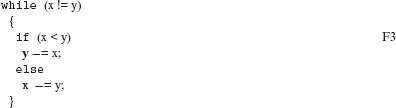
Example 8.30   Consider the following program fragment:

Application of STRP to the above statement generates a total of four mutants shown in M2, M3, M4, and M5. Test cases that distinguish all these four mutants are sufficient to guarantee that all four statements in F3 have been executed at least once.

If STRP is used with the RAP set to include the entire program, the tester will be forced to design test cases that guarantee that all statements have been executed. Failure to design such a test set implies that there is some unreachable code in the program.

 

Trap on if Condition

 

The STRI mutation operator is designed to provide branch analysis for any if-statements in P. When used in addition to the STRP, SSWM, and SMTT operators, complete branch analysis can be performed. STRI generates two mutants for each if statement.

Example 8.31   The two mutants generated for statement if (e)S are as follows:

Here ν is assumed to be a new scalar identifier not declared in P.

The type of ν is the same as that of e.

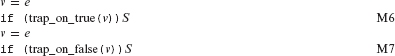
When trap_on_true (trap_on_false) is executed, the mutant is distinguished if the function argument value is true (false). If the argument value is not true (false), then the function returns false (true) and the mutant execution continues.

The STRI operator encourages the tester to generate test cases so that each branch specified by an if statement in P, is exercised at least once. For an implementor of a mutation-based tool, it is useful to note that STRI provides partial branch analysis for if statements. For example, consider a statement of the form: if (c) S₁ else S₂. The STRI operator will have this statement replaced by the following statements to generate two mutants.

• if (c) trap_on_statement() else S₂
• if (c) S₁ else trap_on_statement()

Distinguishing both these mutants implies that both the branches of the if-else statement have been traversed. However, when used with a if statement without an else clause, STRI may fail to provide coverage of both the branches.

 

Statement Deletion

 

SSDL is designed to show that each statement in Ρ has an effect on the output. SSDL encourages the tester to design a test set that causes all statements in the RAP to be executed and generates outputs that are different from the program under test. When applied on P, SSDL systematically deletes each statement in RLS(f).

Example 8.32   When SSDL is applied to F3, four mutants are generated as shown in M8, M9, M10, and M1l.

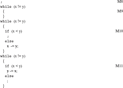
To maintain the syntactic validity of the mutant, SSDL ensures that the semicolons are retained when a statement is deleted. In accordance with the syntax of C, the semicolon appears only at the end of (i) expression-statement and (ii) do-while iteration-statement. Thus, while mutating an expression-statement, SSDL deletes the optional expression from the statement, retaining the semicolon. Similarly, while mutating a do-while iteration-statement, the semicolon that terminates this statement is retained. In other cases, such as the selection-statement, the semicolon automatically gets retained as it is not a part of the syntactic entity being mutated.

 

return Statement Replacement

When a function f executes on test case t, it is possible that due to some fault in the composition of f, certain suffixes of E(f, t) do not affect the output of P. In other words, a suffix may not be a DES of P_f(t) with respect to f ' obtained by replacing an element of RLS(f) by a return. The SRSR operator models such faults.

If E(f, t) = s^m₁ R, then there are m + 1 possible suffixes of E(f, t). These are enumerated below:

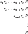
In case f consists of loops, m could be made arbitrarily large by manipulating the test cases. The SRSR operator creates mutants that generate a subset of all possible PMES’s of E(f, t).

Let R₁,R₂, . . . ,R_k be the k return statements in f . If there is no such statement, a parameterless return is assumed to be placed at the end of the text of f. Thus, for our purpose, k ≥ 1. The SRSR operator will systematically replace each statement in RLS(f) by each one of the k return statements. The SRSR operator encourages the tester to generate at least one test case that ensures that E^s(f, i) is a DES for the program under test.

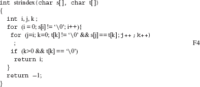
Example 8.33   Consider the following function definition:

/* This is an example from p 69 of Kernighan and Ritichie’s book.*/

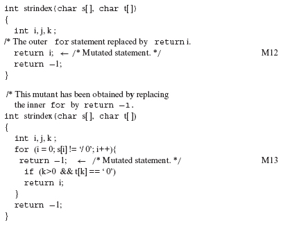
A total of six mutants are generated when the SRSR operator is applied to strindex., two of which are Μ12 and Μ13.

Note that both Μ12 and Μ13 generate the shortest possible PMES for f.

 

goto Label Replacement

In some function f, the destination of a goto may be incorrect. Altering this destination is expected to generate an execution sequence different from E(f , t). Suppose that goto L and goto M are two goto statements in f. We say that these are two goto statements are distinct if L and M are different labels. Let goto l₁, goto l₂, . . ., goto l_n be n distinct goto statements in f. The SGLR operator systematically mutates label l_i in goto l_i to (n – 1) labels l₁, l₂, . . . , l_i−1, l_i+1, . . . , l_n. If n=1, no mutants are generated by SGLR.

 

continue Replacement by break

A continue statement terminates the current iteration of the immediately surrounding loop and initiates the next iteration. Instead of the continue, the programmer might have intended a break that forces the loop to terminate. This is one fault modeled by SCRB. Incorrect placement of continue is another fault that SCRB expects to reveal. SCRB replaces the continue statement by break.

 

Given S that denotes the innermost loop that contains the continue statement, the SCRB operator encourages the tester to construct a test case t to show that E(S,*) is a DES for P_s(t) with respect to the mutated S.

 

break Replacement by continue

 

Using break instead of a continue or misplacing a break are the two faults modeled by SBRC. The break statement is replaced by continue. If S denotes the innermost loop containing the break statement, then SBRC encourages the tester to construct a test case t to show that E(S, t) is a DES for P_s(t) with respect to S', where S' is a mutant of S.

 

Break Out to nth Enclosing Level

 

Execution of a break inside a loop forces the loop to terminate. This causes the resumption of execution of the outer loop, if any. However, the condition that caused the execution of break might be intended to terminate the execution of the immediately enclosing loop, or in general, the n^th enclosing loop. This is the fault modeled by SBRn.

Let a break (or a continue) statement be inside a loop nested n levels deep. A statement with only one enclosing loop is considered to be nested one level deep. The SBRn operator systematically replaces break (or continue) by the function break_out_to_level_n(j), for 2 ≤ j ≤ n. When a SBRn mutant executes, the execution of the mutated statement causes the loop, inside which the mutated statement is nested, and the j enclosing loops, to terminate.

Let S' denote the loop immediately enclosing a break or a continue statement and nested n, n > 0, levels inside the loop S in function f. The SBRn operator encourages the tester to construct a test case t to show that E^S(S, t) is a DES of f with respect to P_f(t) and the mutated S. The exact expression for E(S, t) can be derived for f and its mutant from the execution sequence construction rules listed in Section 8.10.3.

The SBRn operator has no effect on the following constructs:

• break or continue statements that are nested only one level deep.
• A break intended to terminate the execution of a switch statement. Note that a break inside a loop nested in one of the cases of a switch, is subject to mutation by SBRn and SBRC.

Continue Out to nth Enclosing Level

 

This operator is similar to SBRn. It replaces a nested break or a continue by the function continue_out_to_level_n(j), 2 ≤ j ≤ n.

The SCRn operator has no effect on the following constructs:

• break or continue statements that are nested only one level deep.
• A continue statement intended to terminate the execution of a switch statement. Note that a continue inside a loop nested in one of the cases of a switch is subject to mutation by SCRn and SCRB.

while Replacement by do-while

 

Though a rare occurrence, it is possible that a while is used instead of a do-while. The SWDD operator models this fault. The while statement is replaced by the do-while statement.

Example 8.34   Consider the following loop:

 

/* This loop is from p 69 of Kernighan and Ritchie’s book. */

When the SWDD operator is applied, the above loop is mutated to the following.

do-while Replacement by while

 

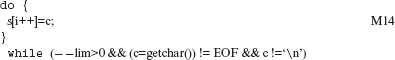
The do-while statement may have been used in a program when the while statement would have been the correct choice. The SDWD operator models this fault. A do-while statement is replaced by a while statement.

Example 8.35   Consider the following do-while statement in P:

/* This loop is from p 64 of Kernighan and Ritchie’s book.*/

It is mutated by the SDWD operator to the following loop.

Notice that the only test data that can distinguish the above mutant is one that sets n to 0 immediately prior to the loop execution. This test case ensures that E(S, *), S being the original do-while statement, is a DES for P_s(t) with respect to the mutated statement, i.e. the while statement.

 

Multiple Trip Trap

 

For every loop in P, we would like to ensure that the loop body satisfied the following two conditions:

• C1: the loop has been executed more than once.
• C2: the loop has an effect on the output of P.

The STRP operator replaces the loop body with the trap_on_statement. A test case that distinguishes such a mutant implies that the loop body has been executed at least once. However, this does not ensure two conditions mentioned above. The SMTT and SMTC operators are designed to ensure C1 and C2.

The SMTT operator introduces a guard in front of the loop body. The guard is a logical function named trap_after_n^th_loop_iteration(n). When the guard is evaluated the n^th time through the loop, it distinguishes the mutant. The value of n is decided by the tester.

Example 8.36   Consider the following for statement:

 

/* This loop is taken from p 87 of Kernighan and Ritchie’s book. */

Assuming that n = 2, this will be mutated by the SMTT operator to the following.

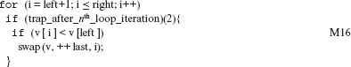
For each loop in the program under test, the SMTT operator encourages the tester to construct a test case so that the loop is iterated at least twice.

 

Multiple Trip Continue

 

An SMTT mutant may be distinguished by a test case that forces the mutated loop to be executed twice. However, it does not ensure condition C2 mentioned earlier. The SMTC operator is designed to ensure C2.

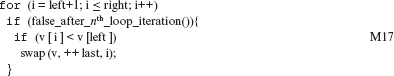
SMTC introduces a guard in front of the loop body. The guard is a logical function named false_after_n^th_loop_iteration(n). During the first n iterations of the loop, false_after_n^th_loop_iteration() evaluates to true, thus letting the loop body execute. During the (n + l)^th and subsequent iterations, if any, it evaluates to false. Thus a loop mutated by SMTC will iterate as many times as the loop condition demands. However, the loop body will not be executed during the second and any subsequent iteration.

Example 8.37   The loop in F7 is mutated by the SMTC operator to the loop in Μ17.

The SMTC operator may generate mutants containing infinite loops. This is specially true when the execution of the loop body effects one or more variables used in the loop condition.

For a function f, and each loop S in RAP(f), SMTC encourages the tester to construct a test case t which causes the loop to be executed more than once such that E(f, t) is a DES of P_f(t)with respect to the mutated loop. Note that SMTC is stronger than SMTT. This implies that a test case that distinguishes an SMTC mutant for statement S, will also distinguish an SMTT mutant of S.

 

Sequence Operator Mutation

 

Use of the comma operator results in the left to right evaluation of a sequence of expressions and forces the value of the rightmost expression to be the result. For example, in the statement f (a, (b = 1, b + 2), c), function f has three parameters. The second parameter has the value 3. The programmer may use an incorrect sequence of expressions thereby forcing the incorrect value to be the result. The SSOM operator is designed to model this fault.

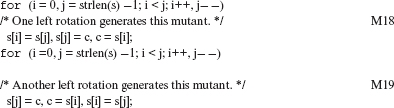
Let e₁, e₂, . . . , e_n denote an expression consisting of a sequence of n sub-expressions. According to the syntax of C, each e_i can be an assignment-expression separated by the comma operator. The SSOM operator generates (n – 1) mutants of this expression by rotating left the sequence one sub-expression at a time.

Example 8.38   Consider the following statement:

/* This loop is taken from p 63 of Keringuan and Ritchie’s book. */

The following two mutants are generated when the SSOM operator is applied on the body of the above loop.

When SSOM is applied to the for statement in the above program, it generates two additional mutants, one by mutating the expression (i = 0, j = strlen(s) – 1 ) to (j = strlen (s) – 1 , i = 0), and the other by mutating the expression (i++, j– –) to (j– –, i++).

The SSOM operator is likely to generate several mutants equivalent to the parent. The mutants generated by mutating the expressions in the for statement in the above example, are equivalent. In general, if the subexpressions do not depend on each other then the mutants generated will be equivalent to their parent.

 

Move Brace Up or Down

 

The closing brace (}) is used in C to indicate the end of a compound statement. It is possible for a programmer to incorrectly place the closing brace thereby including, or excluding, some statements within a compound statement. The SMVB operator models this fault.

 

A statement immediately following the loop body is pushed inside the body. This corresponds to moving the closing brace down by one statement. The last statement inside the loop body is pushed out of the body. This corresponds to moving the closing brace up by one statement.

A compound statement that consists of only one statement may not have explicit braces surrounding it. However, the beginning of a compound statement is considered to have an implied opening brace and the semicolon at its end is considered to be an implied closing brace. To be precise, the semicolon at the end of the statement inside the loop body is considered as a semicolon followed by a closing brace.

 

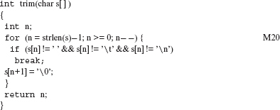
Example 8.39   Consider again the function trim from Kernighan and Ritchie’s book.

 

/* This function is from Kernighan and Ritchie’s book. */

The following two mutants are generated when trim is mutated using the SMVB operator.

/* This is a mutant generated by SMVB. In this one, the for loop body extends to include the s [n+1 ] = ’’ statement. */

/* This is another mutant generated by SMVB. In this one the for loop body becomes empty. */

In certain cases, moving the brace may include, or exclude, a large piece of code. For examp le, suppose that a while loop with a substantial amount of code in its body, follows the closing brace. Moving the brace down will cause the entire while loop to be moved into the loop body that is being mutated. A C programmer is not likely to make such an error. However, there is a good chance of such a mutant being distinguished quickly during mutant execution.

 

Switch Statement Mutation

 

Errors in the formulation of the cases in a switch statement are modeled by SSWM. The expression e in the switch statement is replaced by the trap_on_case function. The input to this function is a condition formulated as e = a, where a is one of the case labels in the switch body. This generates a total of n mutants of a switch statement assuming that there are n case labels. In addition, one mutant is generated with the input condition for trap_on_case set to e = d, where d is computed as d = e! = c₁&&e! = c₂&&. . . e! = c_n. The next example exhibits some mutants generated by SSWM.

 

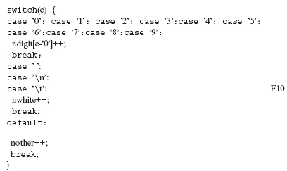
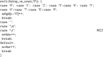
Example 8.40   Consider the following program fragment:

 

/* This fragment is from a program of Kernighan and Ritchie’s book.

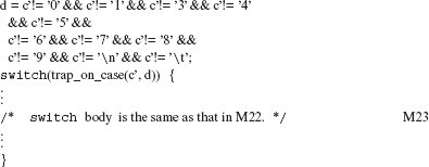
The SSWM operator will generate a total of 14 mutants for F10. Two of them appear in M22 and M23.

c’=c; /* This is to ensure that side effects in c occur once. */

A test set that distinguishes all mutants generated by SSWM ensures that all cases, including the default case, have been covered. We refer to this coverage as case coverage. Note that the STRP operator may not provide case coverage especially when there is fall-through code in the switch body. This also implies that some of the mutants generated when STRP mutates the cases in a switch body, may be equivalent to those generated by SSWM.

Example 8.41   Consider the following program fragment:

 

/* This is an example of fall-through code. */

One of the mutants generated by STRP when applied on Fll will have the putc(’ ’) in the second case replaced by trap_on_statement(). A test case that forces the expression c to evaluate to ‘ ’ and n evaluate to any value not equal to 1, is sufficient to kill such a mutant. On the contrary, an SSWM mutant will encourage the tester to construct a test case that forces the value of c to be ’ ’.

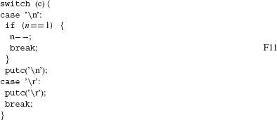
It may, however, be noted that both the STRP and the SSWM serve different purposes when applied on the switch statement. Whereas SSWM mutants are designed to provide case coverage, mutants generated when STRP is applied to a switch statement, are designed to provide statement coverage within the switch body.

8.10.11  Mutating program variables

Incorrect use of identifiers can often induce program faults that remain unnoticed for quite long. Variable mutations are designed to model such faults. Table 8.7 lists all variable mutation operators for C.

 

Scalar Variable Reference Replacement

 

Use of an incorrect scalar variable is the fault modeled by the two mutant operators: VGSR and VLSR. VGSR mutates all scalar variable references by using GS'_f as the range. VLSR mutates all scalar variable references by using LS'_f as the range of the mutation operator. Types are ignored during scalar variable replacement. For example, if i is an integer and x a real, i will be replaced by x and vice versa.

Entire scalar references are mutated. For example, if screen is as declared in Example 8.26, and screen . p1. x is a reference, then the entire reference, i.e. screen . p1. x, will be mutated. p1 or x will not be mutated separately by any one of these two operators. The individual components of a structure may be mutated by the VSCR operator. screen itself may be mutated by one of the strucuture reference replacement operators. We often say that an entity x may be mutated by an operator. This implies that there may be no other entity y to which x can be mutated. Similarly, in a reference such as *p, for p as declared above, *p will be mutated. p alone may be mutated by one of the pointer reference replacement operators. As another example, the entire reference q [i] will be mutated, q itself may be mutated by one of the array reference replacement operators.

 

Table 8.7 List of mutation operators for variables in C.

Mutop	Domain	Description
VASM	Array subscript	Array reference subscript mutation
VDTR	Scalar reference	Absolute value mutation
VGAR	Array reference	Mutate array references using global array references
VGLA	Array reference	Mutate array references using both global and local array references
VGPR	Pointer reference	Mutate pointer references using global pointer references
VGSR	Scalar reference	Mutate scalar references using global scalar references
VGTR	Structure reference	Mutate structure references using global structure references
VLAR	Array reference	Mutate array references using local array references
VLPR	Pointer reference	Mutate pointer references using local pointer references
VLSR	Scalar reference	Mutate scalar references using local scalar references
VLTR	Structure reference	Mutate structure references using local structure references
VSCR	Structure component	Structure component replacement
VTWD	Scalar expression	Twiddle mutations

Array Reference Replacement

 

Incorrect use of an array variable is the fault modeled by two mutation operators: VGAR and VLAR. These operators mutate an array reference in function f using, respectively, the sets GA'_f and LA'_f. Types are preserved while mutating array references. Here, name equivalence of types as defined in C is assumed. Thus, if a and b are, respectively, arrays of integers and pointers to integers, a will not be replaced by b and viceversa.

8.10.12  Structure Reference Replacement

Incorrect use of structure variables is modeled by two mutation operators VGTR and VLTR. These operators mutate a structure reference in function f using, respectively, the sets GT'_f and LT'_f . Types are preserved while mutating structures. For example, if s and t denote two structures of different types then s will not be replaced by t and viceversa. Again, name equivalence is used for types as in C.

 

Pointer Reference Replacement

 

Incorrect use of a pointer variable is modeled by two mutation operators VGPR and VLPR. These operators mutate a pointer reference in function f using, respectively, the sets GP'_f and LP'_f. Types are preserved while performing mutation. For example, if p and q are pointers to an integer and structure, respectively, then p will not be replaced by q, and viceversa.

 

Structure Component Replacement

 

Often one may use the wrong component of a structure. VSCR models such faults. Here, structure refers to data elements declared using the struct type specifier. Let s be a variable of some structure type. Let s.c₁.c₂ . . . .c_n be a reference to one of its components declared at level n within the structure. c_i, 1 ≤ i ≤ n, denotes an identifier declared at level i within s. VSCR systematically mutates each identifier at level i by all the other type compatible identifiers at the same level.

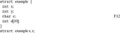
Example 8.42   Consider the following structure declaration:

Reference s.x will be mutated to s.y and s.c by VSCR. Another reference s.d[j] will be mutated to s.x, s.y, and s.c. Note that the reference to s itself will be mutated to r by one of VGSR or VLSR operators.

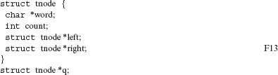
Next, suppose that we have a pointer to example declared as struct example *p; A reference such as p–>x will be mutated to p–>y and p–>c. Now, consider the following recursive structure:

A reference such as q–>left will be mutated to q–>right. Note that left, or any field of a structure, will not be mutated by VGSR or by VLSR operators. This is because a field of a structure does not belong to any of the global or local sets, or reference sets, defined earlier. Also, a reference such as q–>count will not be mutated by VSCR because there is no other compatible field in F13.

 

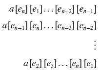
Array reference subscript mutation

 

While referencing an element of a multidimensional array, the order of the subscripts may be incorrectly specified. VASM models this fault. Let a denote an n-dimensional array, n > 1. A reference such as a [e₁][e₂] . . . [e_n] with e_t, 1 ≤ i ≤ n, denoting a subscript expression, will be mutated by rotating the subscript list. Thus, the above reference generates the following (n – 1) mutants when VASM is applied:

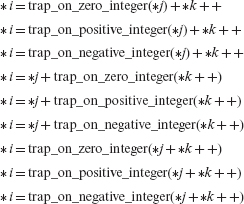
Domain traps

 

The VDTR operator provides domain coverage for scalar variables. The domain partition consists of three subdomains: one containing negative values, one containing a zero, and one containing only the positive values.

VDTR mutates each scalar reference x of type t in an expression, by f(x), where f could be one of the several functions shown in Table 8.8. Note that all functions listed in Table 8.8 for a type t are applied on x. When any of these functions is executed, the mutant is distinguished. Thus, if i, j, and k are pointers to integers, then the statement *i = *j + *k ++ is mutated by VDTR to the following statements.

 

Table 8.8 Functions used by the VDTR operator.

Function † introduced	Description
trap_on_negative_x	Mutant distinguished if argument is negative, else return argument value.
trap_on_positive_x	Mutant distinguished if argument is positive, else return argument value.
trap_on_zero_x	Mutant distinguished if argument is zero, else return argument value.

† x can be integer, real, or double. It is integer if the argument type is int, short, signed, or char. It is real if the argument type is float. It is double if the argument is of type double or long.

 

In the above example, *k ++ is a reference to a scalar, therefore the trap function has been applied to the entire reference. Instead, if the reference was (*k)+ +, then the mutant would be f(*k)++,f being any of the relevant functions.

 

Twiddle mutations

 

Values of variables or expressions can often be off the desired value by ±1. The twiddle mutations model such faults. Twiddle mutations are useful for checking boundary conditions for scalar variables.

 

Each scalar reference x is replaced by pred(x) and succ(x), where pred and succ return, respectively, the immediate predecessor and the immediate successor of the current value of the argument. When applied to a float argument, a small value is added (by succ) to, or subtracted (by pred) from, the argument. This value can be user defined, such as ±.01, or may default to an implementation defined value.

Example 8.43   Consider the assignment: p = a + b Assuming that p, a, and b are integers, VTWD will generate the following two mutants.

Pointer variables are not mutated. However, a scalar reference constructed using a pointer is mutated as defined above. For example, if p is a pointer to an integer, then *p is mutated. Some mutants may cause overflow or underflow faults implying that they are distinguished.

8.11  Mutation Operators for Java

Java, like many others, is an object-oriented programming language. Any such language provides syntactic constructs to encapsulate data and procedures into objects. Classes serve as templates for objects. Procedures within a class are commonly referred to as methods. A method is written using traditional programming constructs such as assignments, conditionals, and loops.

The existence of classes, and the inheritance mechanism in Java, offers a programmer ample opportunities to make mistakes that end up in program faults. Thus the mutation operators for mutating Java programs are divided into two generic categories: traditional mutation operators and class mutation operators.

 

Mutation operators for Java have evolved over a period and are a result of research contributions of several people. The specific set of operators discussed here was proposed by Yu-Seung Ma, Tong-rae Kwon, and Jeff Offutt. We have decided to describe the operators proposed by this group as these operators have been implemented in the μJava (also known as muJava system) mutation system discussed briefly in Section 8.15. Sebastian Danicic from Goldsmiths College University of London has also implemented a set of mutation operators in a tool named Lava. Mutation operators in Lava belong to the “traditional mutation operators” category described in Section 8.11.1. Yet another tool named Jester, developed by Ivan Moore, has another set of operators that also fall into the “traditional mutation operators” category.

Though a large class of mutation operators developed procedural languages such as Fortran and C are applicable to Java methods, a few of these have been selected and grouped into the “traditional” category. Mutation operators specific to the object-oriented paradigm and Java syntax are grouped into the “class mutation operators” category.

The five mutation operators in the “traditional” category are listed in Table 8.9. The class related mutation operators are further subdivided into inheritance, polymorphism and dynamic binding, method overloading, OO, and Java-specific categories. Operators in these four categories are listed in Tables 8.9 through 8.13. We will now describe the operators in each class with examples. We use the notation

to indicate that mutant operator MutOp when applied to program segment Ρ creates mutant Q as one of the several possible mutants.

 

8.11.1  Traditional mutation operators

Arithmetic expressions have the potential of producing values that are not expected by the code that follows. For example, an assignment x = y + z might generate a negative value for x, which causes a portion of the following code to fail. The ABS operator generates mutants by replacing each component in an arithmetic expression by its absolute value. Mutants generated for x = y + z are are follows:

 

Table 8.9 Mutation operators for Java that model faults due to common programming mistakes made in procedural programming.

Mutop	Domain	Description
ABS	Arithmetic expressions	Replaces an arithmetic expression e by abs(e).
AOR	Binary arithmetic operator	Replaces a binary arithmetic operator by another binary arithmetic operator valid in the context.
LCR	Logical connectors	Replaces a logical connector by another.
ROR	Relational operator	Replaces a relational operator by another.
UOI	Arithmetic or logical expressions	Insert a unary operator such as the unary minus or the logical not.

The remaining traditional operators for Java have their correspondence with the mutation operators for C. The AOR operator is similar to OAAN, LCR to OBBN, ROR to ORRN, and UOI to OLNG and VTWD. Note that two similar operators, when applied to programs in different languages, will likely generate a different number of mutants.

8.11.2  Inheritence

Subclassing can be used in Java to hide methods and variables. A subclass C can declare variable x, hiding its declaration, if any, in parent(C). Similarly, C can declare a method m hiding its declaration, if any, in parent(C). The IHD, IHI, IOD, and IOP operators model faults that creep into a Java program due to mistakes in redeclaration of class variables and methods in a corresponding subclass.

Example 8.44   As shown next, the IHD mutation operator removes the declaration of a variable that overrides its declaration in the parent class.

Removal of the declaration for dist in the subclass exposes the instance of dist in the parent class. The IHI operator does the reverse of this process by adding a declaration as in the following:

 

Table 8.10 Mutation operators for Java that model faults related to inheritance.

Mutop	Domain	Description
IHD	Variables	Removes the declaration of variable x in subclass C if x is declared parent(C).
IHI	Subclasses	Adds a declaration for variable x to a subclass C if x is declared in the parrent(C).
IOD	Methods	Removes declaration of method m from a subclass C if m is declared in parent(C).
IOP	Methods	Inside a subclass, move a call super.M(..) inside method m to the beginning of m, end of m, one statement down in m, and one statement up in m.
IOR	Methods	Given that method f1 calls method f2 in parent(C), rename f2 to f'2 if f2 is overridden by subclass C.
ISK	Accesses to parent class	Replace explicit reference to variable x in parent(C) given that x is overridden in subclass C.
IPC	super calls	Delete the super keyword from the constructor in a subclass C.

As illustrated next, IOD exposes a method otherwise hidden in a subclass through overriding.

As shown below, the IOP operator changes the position of any call to an overridden method made using the super keyword. Only one mutant is shown whereas up to three additional mutants could be created by moving the call to the parent’s version of orbit one statement up, one statement down, at the beginning, and the end of the calling method (see Exercise 8.18).

As shown next, method orbit in class planet calls method check. The IOR operator renames this call to, say, j_check.

Given an object X of type farPlanet, X.orbit ( ) will now invoke the subclass version of check and not that of the parent class. Distinguishing an IOR mutant requires a test case to show that X.orbit ( ) must invoke check of the parent class and not that of the subclass.

The ISK operator generates a mutant by deleting, one at a time, occurrences of the super keyword from a subclass. This forces the construction of a test case to show that indeed the parent’s version of the hidden variable or method is intended in the subclass and not the version declared in the subclass.

Lastly, the IPC operator in the inheritance fault modeling category creates mutants by replacing any call to the default constructor of the parent class.

This completes our illustration of all mutation operators that model faults related to the use of inheritance mechanism in Java. Exercise 8.17 asks you to develop conditions that a test case must satisfy to distinguish mutants created by each operator.

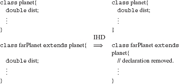
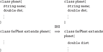
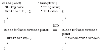
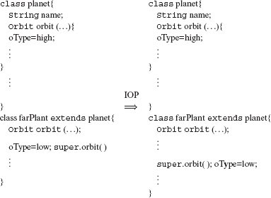
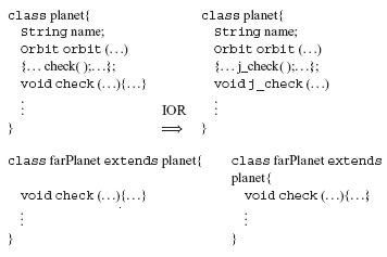
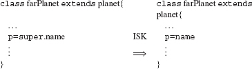
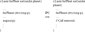
8.11.3  Polymorphism and dynamic binding

Mutation operators related to polymorphism model faults related to Java’s polymorphism features. The operators force the construction of test cases that ensure that the type bindings used in the program under test are correct and the other syntactically possible bindings are either incorrect or equivalent to the ones used.

 

Table 8.11 Mutation operators for Java that model faults related to polymorphism and dynamic binding.

Mutop	Domain	Description
PMC	Object instantiations	Replace type t1 by t2 in object instantiation via new; t1 is the parent type and t2 the type of its subclass.
PMD	Object declarations	Replace type t1 of object x by type t2 of its parent.
PPD	Parameters	For each parameter, replace type t1 of parameter object x by type t2 of its parent.
PRV	Object references	Replace the object reference, e.g. O1, on the right side of an assignment by a reference to a type compatible object reference O2, where both O1 and O2 are declared in the same context.

Table 8.11 lists the four mutation operators that model faults due to incorrect bindings. The following example illustrates these operators.

Example 8.45   Let planet be the parent of class farPlanet. The PMC and PMD mutation operators model the incorrect use of a parent or its subclass as object types. The PPD operator models an incorrect parameter-type binding with respect to a parent and its subclass. Here are sample mutants generated by these two operators.

The PRV operator models a fault in the use of an incorrect object but of a compatible type. The next example illustrates a mutant generated by replacing an object reference on the right side of an assignment by another reference to an object that belongs to a subclass of the object on the left. Here we assume that Element is the parent class of specialElement and gas.

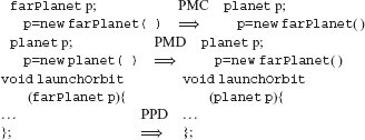
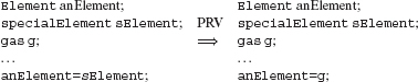
8.11.4  Method overloading

Method overloading allows a programmer to define two or more methods within the same class but with different signatures. The signatures allow a compiler to distinguish between the two methods. Thus a call to an overloaded method m is translated to the appropriate method based on signature matching.

Overloading also offers a programmer an opportunity to make a mistake and use an incorrect method. A compiler will not be able to detect the fault due to such a mistake. The method overloading operators, listed in Table 8.12, are designed to model such faults.

Example 8.46   A mutant generated by the OMR operator forces a tester to generate a test case that exhibits some difference in the behavior of two or more overloaded methods. This is accomplished by replacing the body of each overloaded method with that of another. Here is a sample overloaded method and the two OMR mutants.

 

Table 8.12 Mutation operators for Java that model faults related to method overloading.

Mutop	Domain	Description
OMR	Overloaded methods	Replace body of one overloaded method by that of another.
OMD	Overloaded methods	Delete overloaded method.
OAO	Methods	Change the order of method parameters.
OAN	Methods	Delete arguments in overloaded methods.

The OMD operator generates mutants by deleting overloaded methods one at a time. Test adequate with respect to OMD mutants ensures complete coverage of all overloaded methods. Note that some of the OMD mutants might fail to compile (Can you see why ?). Here is a sample program and one of its two OMD mutants.

Two overloaded methods might have the same number of parameters but possess a different signature. This raises the potential for a fault in the use of an overloaded method. The OAO operator models this fault and generates mutants by changing the parameter order given that the mutant so created is syntactically valid.

Note that in case of three parameters, more than one OAO mutant might be generated. An overloaded method with fewer (or more) parameters might be used instead of a larger (or fewer) number of parameters. This fault is modeled by the OAN operator.

Again, note that the generated mutant must be syntactically valid. Furthermore, one could think of at least two mutants of the call to the getOrbit method, only one of which is shown here.

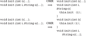
8.11.5  Java specific mutation operators

A few additional operators model Java language specific faults and common programming mistakes. Eight such operators are listed in Table 8.13.

 

The JTD operator deletes this keyword. This forces a tester to show that indeed the variable or method referenced via this was intended. The JSC operator removes or adds the static keyword to model faults related to the use of instance verses class variables. The JID operator removes any initializations of class variables to model variable initialization faults. The JDC operator removes programmer implemented constructors. This forces a tester to generate a test case that demonstrates the correctness of the programmer supplied constructors.

Four operators model common programming mistakes. Using an object reference instead of the content of an object is a fault modeled by the EOA operator.

Example 8.47   The EOA operator models the mistake illustrated next.

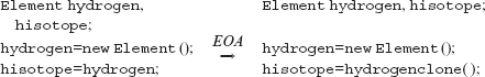
There exists potential for a programmer to invoke an incorrect accessor or a modifier method. These faults are modeled by the EAM and EMM operators, respectively. The accessor (modifier) methods names are replaced by some other existing name of an accessor (modifier) method that matches its signature.

 

Table 8.13 Mutation operators for Java that model language specific and common faults.

Mutop	Domain	Description
JTD	this	Delete this keyword.
JSC	Class variables	Change a class variable to an instance variable.
JID	Member variables	Remove the initialization of a member variable.
JDC	Constructors	Remove user-defined constructors.
EOA	Object references	Replace reference to an object by its contents using clone( ).
EOC	Comparison expressions	Replace = = by equals.
EAM	Calls to accessor methods	Replace call to an accessor method by a call to another compatible accessor method.
EMM	Calls to modifier methods	Replace call to a modifier method by a call to another compatible modifier method.

Example 8.48   The following two examples illustrate the EAM and EMM operators.

8.12   Comparison of Mutation Operators

C has a total of 77 mutation operators compared to 22 for Fortran 77, hereafter referred to as Fortran, and 29 for Java. Note that the double appearance of the number 77 is purely coincidental. Table 8.14 lists all the Fortran mutation operators and the corresponding semantically nearest C and Java operators.

 

Fortran is one of the earliest languages for which mutation operators were designed by inventors of program mutation and their graduate students. Hence the set of 22 operators for Fortran is often referred to as “traditional mutation operators.”

Recall from Section 8.5.2 that there is no perfect, or optimal, set of mutation operators for any language. Design of mutation operators is an art as well as a science. Thus one could always justifiably come up with a mutation operator not presented in this chapter. With this note of freedom, let us now take a comparative look at the sets of mutation operators designed and implemented for Fortran, C, and Java, and understand their similarities and differences.

 

1. Empirical studies have shown that often a small set of mutation operators is sufficient to obtain a strong test set capable of detecting a large number of program faults. For example, in one study, mutants generated by applying only the ABS and ROR operators to five programs were able to detect 87.67% of all faults.

   Similar data from several empirical studies has led to the belief that mutation testing can be performed efficiently and effectively, using only a small set of operators. This belief is reflected in the small set of five traditional mutation operators for Java. While each one of the operators listed in Table 8.14 can be used to mutate Java programs, several have not been included in the set listed in Section 8.11.

2. C has many more primitive types than Fortran. Further, types in C can be mixed in a variety of combinations. This has resulted in a large number of mutation operators in C that model faults related to an incorrect use of an operator in a C program. Similar mistakes can also be made by a Java programmer, such as the replacement of the logical and operator (&&) by another version (&) that forces both operands to be evaluated. Hence, several mutation operators that mutate the operators in a C expression are also applicable to Java programs. The Lava mutation system does include an extensive set of operator mutations.

    

   Table 8.14 A comparison of mutation operators proposed for Fortran, C, and Java.

   

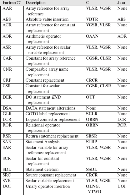
   Certainly, many of the C operators that could be used to mutate Java programs are not included in Java. The OEAA operator is one such example; others can be found by browsing through the mutation operators listed in Section 8.10.

3. The statement structure of C is recursive. Fortran has single line statements. Though this has not resulted in more operators being defined for C, it has, however, made the definition of operators such as SSDL and SRSR significantly different from the definition of the corresponding operators in Fortran. Java does not include such statement mutations.
4. Scalar references in C can be constructed non-trivially using functions, pointers, structures, and arrays. In Fortran, only functions and arrays can be used to construct scalar references. This has resulted in operators such as VSCR and several others in the variable replacement category. Note that in Fortran, SVR is one operator whereas in C, it is a set of several operators.
5. C has a comma operator that is not in Fortran. This has resulted in the SSOM operator. This operator is not applicable to Java.
6. All iterations, or the current iteration, of a loop can be terminated in C using, respectively, the break and continue statements. Fortran provides no such facility. This has resulted in additional mutant operators such as SBRC, SCRB, and SBRn. Java also provides the break and continue statements and hence these operators are valid for Java.
7. The inter-class mutation operators for Java are designed to mutate programs written in object-oriented languages and hence are not applicable to Fortran and C. Of course, some of these operators are Java specific.

8.13  Mutation Testing within Budget

The test adequacy criteria provided by mutation has been found experimentally to be the most powerful of all the existing test adequacy criteria. This strength of mutation implies that given a test set adequate with respect to mutation, it is very likely to be adequate with respect to any other adequacy criterion as well. It also implies that if a test set has been found adequate with respect to some other adequacy criterion, then it is not adequate with respect to some mutation-based adequacy criterion. Note that the adequacy criterion provided by mutation depends on the mutation operators used the more the operators used, the stronger is the criterion assuming that the operators are chosen carefully.

 

The strength of mutation does not come for free. Let C_A be the cost of developing a test set adequate with respect to criterion A. One component of C_A is the time spent by testers in obtaining an A-adequate test set for the application under test. Another component of C_A is the time spent in the generation, compilation, and execution of mutants. C_mut, the cost of mutation, turns out to be much greater than C_A for almost any other path oriented adequacy criterion A. We need strategies to contain C_mut to within our budget.

There are several strategies available to a tester to reduce C_mut and bring it down to an acceptable level within an organization. Some of these options are exercised by the tester while others by the tool used for assessment. Here we briefly review two strategies that have been employed by testers to reduce the cost of mutation testing. The strategy of combining mutants into one program to reduce compilation, and executing the combined program in parallel, to reduce the total execution time, have been proposed and are alluded to only in the bibliography section.

8.13.1  Prioritizing functions to be mutated

Suppose that you are testing an application Ρ that contains a large number of classes. It is recommended that you prioritize the classes such that classes that support the most critical features of the application receive higher priority than others. If your application is written in a procedure oriented language such as C, then prioritize the functions in terms of their use in the implementation of critical features. Note that one or more classes, or one or more functions, might be involved in the implementation of a feature. Figure 8.3 illustrates class prioritization based on the criticality of features.

 

Now suppose that T_P is the test whose adequacy is to be assessed. We assume that Ρ behaves in accordance with its requirements when tested against T_P. Use the mutation tool to mutate only the highest priority classes. Now apply the assessment procedure shown in Figure 8.1. At the conclusion of this procedure, you would have obtained the mutation score for T_P with respect to the mutated class. If T_P is found adequate then you could either terminate the assessment procedure or repeat the procedure by mutating the classes with the next highest priority. If T_P is not adequate then you need to construct T'_p by adding tests to T_P so that T'_p is adequate.

One can use the above strategy to contain the cost of mutation testing. At the end of the process, you would have developed an extremely reliable test set with respect to the critical features of the application. One major advantage of this strategy is that it allows a test manager to tailor the test process to a given budget. The higher the budget, the more classes you will be able to mutate. This strategy also suggests that mutation testing can be scaled to any sized application by a careful selection of portions of the code to be mutated. Of course, you might have guessed that a similar approach can also be used when measuring adequacy with respect to any code coverage-based criterion.

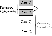
Figure 8.3 Feature F₁ is accorded higher priority than feature F₂. Hence assign higher priority to classes C₁ and C₂ for mutation. Feature priority is based on criticality, i.e. on the severity of damage in case the program fails when executing a feature.

8.13.2  Selecting a subset of mutation operators

Most mutation tools offer a large palette of mutation operators to select from. In an extreme case, you could let the tool apply all operators to the application under test. This is likely to generate an overwhelmingly large set of mutants depending on the size of P. Instead, it is recommended that you select a small subset of mutation operators and mutate only the selected portions of Ρ using these operators. An obvious question is: What subset of mutation operators should one select ?

 

An answer to the question above is found in Table 8.15. The data in this table is based on two sets of independently conducted experiments. One experiment was reported by Jeff Offutt, Greg Rothermel and Christian Zapf in May of 1993. The other experiment was reported in the by Eric Wong in his doctoral thesis published in December of 1993. In both studies it was found that a test set adequate with respect to a small set of mutation operators, listed in the table, is nearly adequate with respect to a much larger set of operators.

 

Offutt and colleagues found that by using the set of five mutation operators in the table, they could achieve an adequacy of greater than 0.99 on all 22 operators listed in Table 8.14. Wong found that using the ABS and ROR operators alone, one could achieve an adequacy of over 0.97 against all 22 operators in Table 8.14. The operators are listed in Table 8.15 in the order of their effectiveness in obtaining a high overall mutation score. Similar results have also been reported earlier and are cited in the bibliography section.

 

Table 8.15 A constrained set of mutation operators sufficient to achieve a mutation score close to 1.

Study	Sufficient set of mutation operators
Offutt, Rothermel, and Zapf	ABS, ROR, LCR, UOI, AOR
Wong	ABS, ROR

The results of the two studies mentioned above suggest a simple strategy: assess the adequacy of your test set against only a small subset of all mutation operators. One might now ask: Why do we need a larger set of operators ? As each mutation operator models a common error, it cannot be considered redundant. However, the two studies mentioned above suggest that some operators are “stronger” than the others in the sense that if a test set distinguishes all mutants generated by these then it will likely distinguish mutants generated by the “weaker” ones.

In practice, the mutation operators applied will depend on the budget. A lower budget test process will likely apply only a few operators than a higher budget process. In a lower budget situation, the operators in Table 8.15 turn out to be a useful set.

8.14  CASE and Program Testing

CASE: Computer-Aided Software Engineering is a collection of methods and tools for software development. There exists a large number of commercial and open source tools that aid in the software development processes.

Figure 8.4 shows the stages of a development process. The arrows indicate a sequence of different development stages. However, for the discussion below, the sequence does not matter and feedback loops in the process are expected. Below are some ways in which mutation can be used during the entire development process.

Requirements gathering: Software testing could begin, and does so in some processes, in the requirements analysis phase. In this phase tests are developed alongside system requirements. As no code is available, it is unlikely that mutation could be used at this point in the development process.

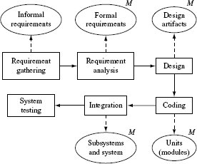
Figure 8.4 Software artifacts generated in a development process. Artifacts that can be subjected to mutation are indicated with an Μ on the upper right corner. Solid arrows indicate flow of the development process. Dashed arrows indicate production of artifacts in the corresponding stage.

Analysis and design: The next step is requirements analysis and design. Depending on the level of formality in this process, the design could be expressed using formal specifications such as in the Ζ language, or as a finite state model, or as a statechart model. In all cases it is possible to apply mutation to the design and generate alternate mutated designs. Tests can be generated, automatically or manually, from the original designs. These tests can then be used to test the mutated designs to ensure the correctness of the original design.

 

Unit development and testing: In a traditional development environment coding could begin soon after the design has been validated via some means, e.g., design reviews. Developers and testers may test test their code at this level using tools such as JUnit, PyUnit, and other unit testing tools. At this point the adequacy of unit tests could be determined using tools such as muJava for Java and Milu for C. The adequacy score can then be used to improve unit tests. Of course as determining an accurate mutation score is a time-consuming task, it should be undertaken only when the unit under test is sufficiently stable and unlikely to change too often.

 

Integration and testing: Units are gradually integrated into subsystems and tested as explained in Chapter 11. At this stage interface mutation could be applied to assess the adequacy of integration tests. Interface mutation focuses only on those elements of a subsystem that correspond to the component interfaces. This reduces the cost of mutation testing.

System testing: Mutation can be applied during system testing though it ought to be done carefully and in a planned manner. Let us assume that a system has been tested and has met the United States Department of Defense DO 178B requirements. For Level C (catastrophic) software these requirements ensure that the tests are MC/DC adequate.

In the above case, one could certainly attempt to apply constrained (or selective) mutation to the entire system and assess the adequacy of the system tests. However, depending on the size and complexity of the system software mutating the entire system might not be practical. In such a situation, it is best to identify portions of the system code that are most critical for reliable system operation (see Section 8.13.1). Only these portions of the code can be subject to mutation. The MC/DC adequate tests that correspond to the selected portion of the code can then be assessed and improved if found necessary.

Agile development: Testing is a nearly continuous activity in an agile development environment and depends, in at least some cases, on customer demands. Thus, customer demand on software reliability, rather than prevalent customs, is a key factor differentiating testing in an agile environment. Nevertheless, when needed mutation can be applied at all stages. However, as mentioned earlier, it should be applied only to stable code regardless of the development stage. The Jumble mutation tool has been designed to be applicable to Java code under test using JUnit in an agile environment.

8.15  Tools

Tool support is essential while assessing the adequacy of tests for even small programs, say, 100 lines of C code. This aspect of mutation testing was known to its original developers. Consequently, research in program mutation was accompanied by the development of prototype or fully operational robust tools.

 

Table 8.16 A partial list of mutation tools developed and their availability.

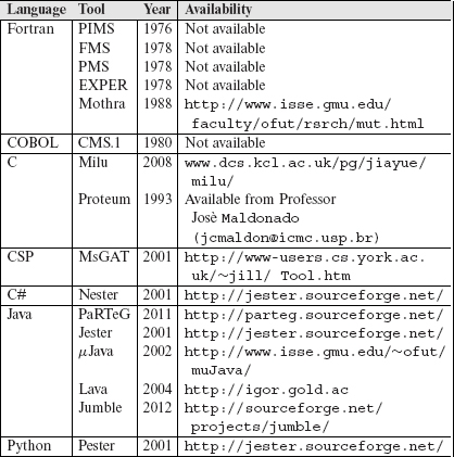
Table 8.16 is a partial list of mutation tools. Some of the tools listed here are now obsolete and replaced by newer versions while others continue to be used or are available for use. Mothra, Proteum, Proteum/IM, μJava, and Lava belong to the latter category. Lava is novel in the sense that it allows the generation of second order mutants; certainly Mothra has also been used in some scientific experiments to generate higher order mutants.

Milu is a new addition to the list of tools for mutation testing. It mutates C programs. It supports both first order and higher order mutations. MILU implements the C mutation operator set designed at Purdue University and summarized in Section 8.10.

Most mutation tools provide support for selecting a subset of the mutation operators to be applied and also the segment of the program under test. These two features allow a tester to perform incremental testing. Test sets could be evaluated against critical components of applications. For example, in a nuclear plant control software, components that relate to the emergency shutdown system could be mutated by a larger number of mutation operators for test assessment.

While mutation testing is preferably done incrementally, it should also be done after the test set to be evaluated has been evaluated against the control flow and data flow metrics. Empirical studies have shown that a test data that is adequate with respect to the traditional control flow criteria, e.g. decision coverage, are not adequate with respect to mutation. Thus there are at least two advantages of applying mutation after establishing control flow adequacy. One, several mutants will likely be distinguished by control-flow adequate tests. Second, the mutants that remain live, will likely help enhance the test set.

In practice, data flow based test adequacy criteria turn out to be stronger than those based on control flow. Again, empirical studies have shown that test sets adequate with respect to the all-uses criterion are not adequate with respect to mutants generated by the ABS and ROR operators. Certainly, this is not true in some cases. However, this suggests that one could apply the ABS and ROR operators to evaluate the adequacy of a test set that is found to be adequate with respect to the all-uses criterion. By doing so, a tester will likely gain the two advantages mentioned above.

 

Exercises

8.1 Given program Ρ in programming language L and a non-empty set Μ of mutation operators, what is the smallest number of mutants generated when mutation operators in Μ are applied tο Ρ?

8.2 (a) Let D and R denote, respectively, the sets of elements in the domain of mutation operator M. Suppose that program Ρ contains exactly one occurrence of each element of D and that D = R. How many mutants of Ρ will be generated by applying Μ ? (b) How might your answer to (a) change if D ≠ R?

8.3 Create at least two mutants of P8.2 that could lead to an incorrect signal sent to the caller of procedure checkTemp. Assume that you are allowed to create mutants by only changing constants, variables, arithmetic operators, and logical operators.

8.4 In Program P8.2, we have used three if statements to set danger to its appropriate value. Instead, suppose we use if-else structure as follows:

 

12 if (highCount = = l) danger=moderate;

13 else if (highCount = =2) danger=high;

14 else if (highCount = = 3) danger=veryHigh;

15 return(danger);

 

Consider mutant M3 of the revised program obtained by replacing veryHigh by none. Would the behavior of M3 differ from that of M1 and M2 in Examples 8.4 and 8.5 ?

8.5 In Example 8.12 the tests are selected in the order t₁, t₂, t₃, t₄. Suppose the tests are selected in the order t₄, t₃, t₂, t₁. By how much will this revised order change the number of mutant executions as compared to the number of executions in Example 8.12 ?

8.6 Why is it considered impossible to construct an ideal set of mutation operators for non-trivial programming languages? Does there exist a language for which such a set can be constructed ?

8.7 Consider the statement: “In mutation testing, an assumption is that programmers make small errors.” Critique this statement in the light of the Competent Programmer Hypothesis and the Coupling Effect.

8.8 Consider Program P8.3 in Example 8.17. Consider three mutants of 8.17 obtained as follows:

 

M₁: At line 4, replace index < size by index < size – 1.

M₂: At line 5, replace atWeight > w by atWeight ≥ w.

M₃: At line 5, replace atWeight > w by atWeight > abs(w).

 

For each of the three mutants, derive a test case that distinguishes it from the parent or prove that it is an equivalent mutant.

8.9 Formulate a “Malicious programmer hypothesis” analogous to the Competant Programmer Hypothesis. In what domain of software testing do you think such a hypothesis might be useful?

8.10 Under weak mutation, a mutant is considered distinguished by a test case t if it satisfies conditions C₁ and C₂ in Section 8.3.4. Derive a minimal sized test set Τ for Program 8.3 that is adequate with respect to weak mutation given the three mutants in Exercise 8.8. Is Τ adequate with respect to strong mutation ?

8.11 As explained in Section 8.3.2, adequacy assessment and test enhancement could be done concurrently by two or more testers. While the testers share a common test database, it might be possible that two or more testers derive tests that are redundant in the sense that a test already derived a by a tester might have distinguished a mutant that some other tester has not been able to distinguish.

Given that adequacy assessment is done by two testers, sketch a sequence of events that reveal the possibility of a redundant test case being generated. You could include events such as: Tester 1 generates mutants, tester 2 executes mutants, Tester 1 adds a new test case to the database, Tester 2 removes a test case from the database, and so on. Assume that (a) tester TS is allowed to remove a test case from the data base but only if it was created by TS and (b) the adequacy assessment process is started all over when a fault is discovered and fixed.

8.12 Consider naming the statement deletion operator for C as: statement replacement by null statement. Why would this be a poor naming choice ?

8.13 Consider the following simple function.

 

1 function xRaisedToy(int x, y){

2 int power=1; count=y;

3 while(count>0){

4 power=power* x;

5 count=count-1;

6 }

7 return(power)

8 }

 

(a) How many abs mutants will be generated when xRaisedToy is mutated by the abs operator ? (b) List at least two abs mutants generated ? (c) Consider the following mutant of xRaisedToy obtained by mutating line 4:

power=power*abs(x):

Generate a test case that distinguishes this mutant, or show that it is equivalent to xRaisedToy.

(d) Generate at least one abs mutant equivalent to xRaisedToy.

8.14 Let T_D denote a decision-adequate test set for the function in Exercise 8.13. Show that there exists a T_D that fails to distinguish the abs mutant in part (c).

8.15 The AMC operator was designed to model faults in Java programs related to the incorrect choice of the access modifiers such as private and public. However, this operator was not implemented in the μJava system. Offer arguments in support of, or against, the decision not to include AMC in μJava.

8.16 Let P_J denote a Java method corresponding to function xRaisedToy in Exercise 8.13. Which Java mutation operators will generate a non-zero number of mutants for P_J given that no other part of the program containing P_J is to be mutated ?

8.17 Derive conditions a test case must satisfy to distinguish each mutant shown in Example 8.44.

8.18 Given the following class declarations, list all mutants generated by applying the IOP operator:

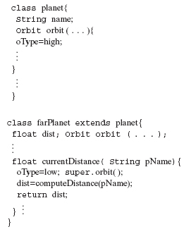
8.19 Consider the following simple program Ρ that contains an error at line 3. A mutant M, obtained by replacing this line as shown, is the correct program. The mutant operator used here replaces a variable by a constant from within the program. In C, this operator is named CRCR. Thus the error in the program is modeled by a mutation operator.

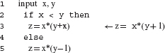
(a) Construct a test case t₁ that causes Ρ to fail and establishes the relation P(t₁) ≠ M(t₁).

(b) Can you construct a test case t₂ on which Ρ is successful but P(t₂) ≠ M(t₂) does not hold ?

(c) Construct a test set Τ that is adequate with respect to decision coverage, MC/DC, and all-uses coverage criteria and that does not reveal the error. Does any test in Τ distinguish Μ from P ?

8.20 As reported by Donald Knuth, missing assignments accounted for over 11% of all the faults found in T_EX. Considering a missing initialization as a special case of missing assignment, these faults account for over 15% of all faults found in T_EX. This exercise illustrates how a missing assignment is detected using mutation. In the program listed next, the position of a missing assignment is indicated. Let P_c denote the correct program.

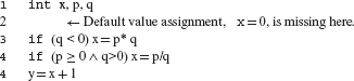
Show that each of the following mutants, obtained by mutating line 3, is error revealing.

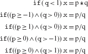
One might argue that the missing initialization above can be detected easily through static analysis. Assuming that the program fragment above is a small portion of a large program, can you argue that static analysis might fail to detect the missing initialization ?

8.21 Example 8.21 illustrates how a simple mutation can reveal a missing condition error. The example showed that the error must be revealed when mutation adequacy has been achieved. Develop test sets T₁, T₂, and T₃ adequate with respect to, respectively, decision coverage, MC/DC, and all-uses coverage criteria such that none of the tests reveals the error in function misCond?

8.22 Some program faults might escape detection using mutation as well as any path oriented testing strategy. Dick Hamlet provides a simple example of one such error. Hamlet’s program is reproduced below.

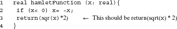
The error is in the use of function sqr, read as “square,” instead of the function sqrt, read as “square root.” Notice that there is a simple mutation that exists in this program, that of sqrt being mutated by the programmer to sqr. However, let us assume that there is no such mutation operator in the mutation tool that you are using. (Of course, in principle, there is nothing which prevents a mutation testing tool from providing such a mutation operator.) Hence, the call to sqr will not be mutated to sqrt.

Consider the test set Τ = {< x = 0 >, < x = – 1 >, < x = 1 >}. It is easy to check that hamletFunction behaves correctly on Τ. Show that Τ is adequate with respect to (a) all path oriented coverage criteria, such as all-uses coverage and MC/DC, and (b) all mutants obtained by using the mutation operators in Table 8.14. It would be best to complete this exercise using a mutation tool. If necessary, translate hamletFunction into C if you have access to Proteum or to Java if you have access to μJava.

8.23 Let Μ be a mutant of program Ρ generated by applying some mutation operator. Suppose that Μ is equivalent to P. Despite the equivalence, Μ might be a useful program, and perform better (or worse) than P. Examine Hoare’s FIND program and its mutant obtained by replacing the conditionl.GT.F, labeled 70, by FALSE. Is the mutant equivalent to its parent ? Does it perform better or worse than the original program ?

8.24 Let MS(X) denote the mutation score of test set X with respect to some program and a set of mutation operators. Let T_A be a test set for application A and U_A ⊆ T_A. Develop an efficient minimization algorithm to construct T'_A = T_A – U_A such that (a) MS(T_A) = MS(T'_A) and (b) for any T'_A ⊂ T_A, |T'_A | < |T''_A|. (Note: Such minimization algorithms are useful in the removal of tests that are redundant with respect to the mutation adequacy criterion. One could construct similar algorithms for minimization of a test set with respect to any other quantitative adequacy criterion.)

8.25 Suppose a class C contains at an overloaded method with three versions. What is the minimum number of mutants generated when the OAN operator is applied to C ?

8.26 The following are believed to be “myths of mutation.” Do you agree?

1. It is an error seeding approach.
2. It is too expensive relative to other test adequacy criteria.
3. It is “harder” than other coverage based test methods in the sense that it requires a tester to think much more while developing a mutation adequate test.
4. It discovers only simple errors.
5. It is applicable only during unit testing.
6. It is applicable only to numerical programs, e.g. a program that inverts a matrix.

8.27 Consider the following program originally due to Jeff Voas, Larry Morell, and Keith Miller.

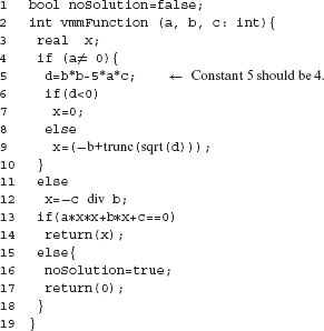
Given inputs a, b, and c, vmmFunction is required to find an integral solution to the quadratic equation a * x² + b * x + c = 0. If an integral solution exists, the program returns with the solution, if not then it sets the global variable noSolution to true and returns a 0. Function vmmFunction has a fault at line 5, constant 5 should instead be 4.

1. Consider the set M_W of mutants created by applying the mutation operators suggested by Wong, as in Table 8.15, to vmmFunction. Is any mutant in M_W error revealing?
2. Now consider the set M_O of mutants created by applying the mutation operators suggested by Offutt, as in Table 8.15, to vmmFunction. Is any mutant in M_O error revealing?
3. Next, suppose that we have fixed the fault at line 5 but line 6 now contains a fault, the faulty condition being d ≤ 0. Is there any error revealing mutant of vmmFunction in M_W ? M_O ? (Note that M_W and M_O are now created by applying the mutation operators to vmmFunction with the fault in the condition at line 6.)

It might be best to do this exercise with the help of a tool such as Proteum or μJava. When using a tool, you will need to translate the pseudo-code of vmmFuntion into C or Java, as appropriate.

8.28 Program P8.4 shows a function named count that is required to read a character and an integer value. If the character input is ‘a’ then the entry a[value] is incremented by one. If the character input is a ‘b’ then entry b[value] is incremented by 1. The input value is ignored for all other characters. The value input must satisfy the condition 0 ≤ value < N.

The function count is supposed to read the input until it gets an end-of-file character, denoted by eof, when it terminates. Arrays a and b are global to the function. Note that as shown here, count does not check if the input value is in its intended range. Thus, an input integer value could force the function, and its container program, to misbehave.

Program P8.4

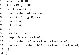
1. Is it possible to develop a test set that is adequate with respect to the MC/DC criterion such that the input integer value is within its intended range in each test case ?
2. Is it possible to develop a test set that is adequate with respect to the all-uses coverage criterion such that the input integer value is within its intended range in each test case ?
3. Is it possible to develop a test set that is adequate with respect to the mutation criterion such that the input integer value is within its intended range in each test case ? Assume that all traditional mutation operators listed in Table 8.14 are used.

8.29 Some programming languages provide the set type. Java provides a SET interface. Specification language Z, functional language Miranda, and procedural language SETL are examples of languages that provide the set type. Consider a mutation operator named SM–abbreviation for set mutation. SM is applied to any object of type set in a specification. Thus, the application of SM to specification S₁ mutates it to another specification S₂ by changing the contents of an object defined as a set.

1. Develop a suitable semantics for SM. Note that traditional mutation operators such as variable replacement will replace an object x of type set with another object y defined in the same program. However, SM is different in that it mutates the value of a set object in a specification.
2. Think of applying SM to a program during execution by mutating the value of a set object when it is referenced. Why would such a mutation be useful ?