
chapter 8
TEST PROCEDURES
Objectives:
After completing this chapter, you can understand the following:
- The definition of parametric and non-parametric tests
- The detailed explanation of ANOVA
- The definition of Mann-Whitney test and its performance in SPSS
- The definition of Kruskal-Wallis test and its step by step procedure in SPSS
- The definition of chi-square test and its test procedure in SPSS statistics
- The definition of multivariate analysis and its test procedure in SPSS-MANOVA
After collecting the data, we need to have ways for analyzing them to retrieve results and facts from it. Researchers are very much interested in analyzing such data. For example, a population of Tigers in India is collected. It may be the total number from reserve forests, tropical forests or plantation forests. From these numbers, how can we say that population of tigers is getting reduced day by day? or How can we say that Bengal Tigers are not distributed throughout the reserve forest? Such questions are answered by the help of test procedures. There are two types of test procedures depending upon the operational content of the data – parametric and non-parametric tests. These two tests are basically based on population of data.
8.1 PARAMETRIC AND NON-PARAMETRIC TESTS
Non-parametric statistics covers those data not belong to any distribution. That is, you can use non-parametric statistics if your measurement scale is nominal or ordinal. Non-parametric statistics are less powerful because they use less information in their calculations. This statistics uses ordinal position of pairs of scores rather than mean or standard deviation. The non-parametric methods are used in study of populations that takes on ranked orders. For example, a survey needs to review a movie by rating from one to five stars. Here, non-parametric methods are easy to be used by the researcher as the population is not much known. Mann-Whitney test, rank sum test and Kruskal-Wallis test are the examples of non-parametric tests.
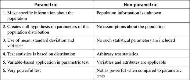
In parametric test, all information about the population is known completely. Also the researcher is aware of which test is suitable for his/her application. The parametric tests use certain assumptions that produce more accurate and precise estimates. Power of the statistics can be used in these types of test and may mislead if the assumptions are not valid. t-test, z-test, f-test and ANOVA are examples of parametric tests. This chapter discusses various test procedures used in research data analysis. Table 8.1 gives major differences between parametric and non-parametric test procedures.
Table 8.1 Difference between parametric and non-parametric tests
8.2 ANOVA
ANOVA stands for Analysis of Variance. It is a statistical model developed by R.A. Fisher to analyze the variations among and between the groups. In ANOVA, we use variance like a quantity to study the equality or non-equality of means of particular populations. There are various test methods available to compare and study the means of two groups, but ANOVA finds importance in those situations where we need to compare the means of more than two groups. Thus, this method is very useful for researchers and scientists in various fields such as biology, statistics, business and education. Using ANOVA, we can infer whether a particular group is drawn from a population whose mean is under investigation. ANOVA is essentially a procedure for testing the difference among different groups of data for homogeneity. If there is a wide variation from its mean, then ignore the particular group from its parent population.
The logic used in ANOVA to compare means of multiple groups is similar to that used with the t-test to compare means of two independent groups. The assumptions needed for ANOVA are as follows:
- Random, independent sampling from the k populations
- Normal population distributions
- Equal variances within the k populations
The first assumption is the real critical one, whereas we can avoid the points 2 and 3, if the sample size is very large.
8.2.1 Tricks and Technique – ANOVA
The stepwise technique for working out ANOVA is as follows:
- Obtain the mean of each sample, i.e., obtain X1, X2, X3, …, Xk when there are k samples.
- Take the deviations of the sample means from the mean of the sample means and calculate the square of such deviations which may be multiplied by the number of items in the corresponding sample, and then obtain their total. This is known as the sum of squares for variance between the samples.
- Divide the result of step (2) by the degrees of freedom between the samples to obtain variance or Mean Square (MS) between samples.
- Obtain the deviations of the values of the sample items for all the samples from corresponding means of the samples and calculate the squares of such deviations and then obtain their total. This total is known as the sum of squares for variance within samples (or SS within).
- Divide the result of step (4) by the degrees of freedom within samples to obtain the variance or MS within samples.
- Now find the total variance, SS for total variance = SS between + SS within
- Finally, find the F-ratio,

8.2.2 One-way and Two-way ANOVA
One-way ANOVA is used to compare means from at least three groups from one variable (Fig. 8.1). The null hypothesis is, “all the population group means are equal” and the alternative hypothesis is, “at least one of the population means differs from the other”. This may seem confusing as we call it as Analysis of Variance even though we are comparing means. Reason of the test statistic uses evidence about two types of variability. We will only consider the reason behind it instead of the complex formula used to calculate it.
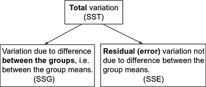
Fig. 8.1 One-way ANOVA
Step-by-Step ANOVA
The method used today for comparisons of three or more groups is called analysis of variance (ANOVA). This method has the advantage of testing whether there are any differences between the groups with a single probability associated with the test. The hypothesis tested is that all groups have the same mean. Before we present an example, notice that there are several assumptions should be met before using the ANOVA.
Essentially, we must have independence between groups (unless a repeated measures design is used); the sampling distributions of sample means must be normally distributed; and the groups should come from populations with equal variances (called homogeneity of variance). The basic principle of ANOVA is to test for differences among means of populations by examining the amount of variation within each of these samples, relative to the amount of variation between the samples.
In short, we have to make two estimates of population variance, viz., one based on between samples variance and the other based on within samples variance. Then the said two estimates of population variance are compared with F-test,
Two-way ANOVA (Fig. 8.2) technique is used when the data are classified on the basis of two factors.
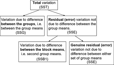
Fig. 8.2 Two-way ANOVA
ANOVA test example
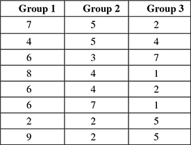
Consider the situation where ANOVA is used for the statistical analysis. The details are given in Table 8.2.
Table 8.2 Group details
The calculated mean and standard deviations can be represented in Table 8.3.
Table 8.3 Mean and standard deviation
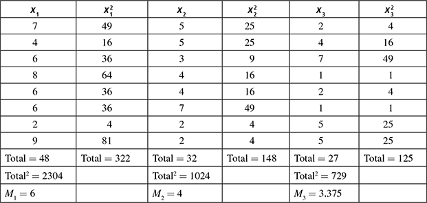
Table 8.4 Significant-probability table
According to the F significant/probability (Table 8.4) with df = (2, 21), F must be at least 3.4668 to reach p ≤ 0.05, so F score is statistically significant. In other words, the hypothesis can be accepted or supported.
8.3 MANN-WHITNEY TEST
The Mann-Whitney U test is the counterpart of the independent sample t-test. It is a non-parametric test of the null hypothesis. The Mann-Whitney U test is used to compare differences between two independent groups when the dependent variable is either ordinal or continuous. For example, one might compare the speed at which two different groups of people can run 100 metres, where one group has trained for six weeks and the other has not. Unlike the independent sample t-test, the Mann-Whitney U test allows to draw different conclusions about the data depending on assumptions of data’s distribution.
Requirements
- Two random, independent samples
- The data is continuous – in other words, it must, in principle, be possible to distinguish between values at the nth decimal place
- Scale of measurement should be ordinal, interval or ratio. For maximum accuracy, there should be no ties, though this test – like others – has a way to handle ties
Null hypothesis: The null hypothesis asserts that the medians of the two samples are identical.
Case Study
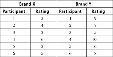
To have more understanding, let us look a basic case study. A general market study of two products under same category is being done. Consider Brand X tea and Brand Y tea. A voting scheme is carried out where each participant can just rate one product and the results need to be compared. Before proceeding, how will we confirm the test that needs to be used is Mann-Whitney?
Here we have two conditions, with each participant taking part in only one of the conditions. The data are ratings (ordinal data), and hence a non-parametric test is appropriate, thus concluding the test to be done is the Mann-Whitney U test. Table 8.5 shows the input obtained from an audience rating of two brands X and Y.
Table 8.5 Audience rating of the brands
Step 1:
Rank all scores together (Table 8.6), ignoring which group they belong to.
Step 2:
Add up the ranks for Brand X, to get T1 and add up the rank for Brand Y, to get T2. The largest rank is selected to work out in the equation

T2 is selected with rank 55.
Step 3:
We have to initialize N and M. These are number of participants in each group, and the number of people in the group that gave the larger rank total. Here, both values are equal to six.
Step 4:
Perform the calculation depending on the formulae,
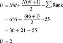
Step 5:
Compare the resultant U, with the critical value of Mann–Whitney test. For our result to be significant, our obtained U has to be equal to or less than this critical value. From the critical table,
The critical value for a two-tailed test at 0.05 significance level = 5
The critical value for a two-tailed test at 0.01 significance level = 2
So, our obtained U is less than the critical value of U for a 0.05 significance level. It is also equal to the critical value of U for a 0.01 significance level.
This means that there is a highly significant difference (p ≤ 0.01) between the ratings given to each brand.
8.3.1 How to Perform Mann-Whitney Test in SPSS?
The Mann-Whitney test can be easily performed in the SPSS software. The following are the series of steps that need to be performed for calculating the Mann-Whitney test.
Go to Analyze > Non-parametric Tests > Legacy Dialogues > 2 Independent Samples … on the top menu, as shown in Fig. 8.3.
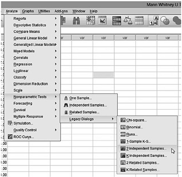
Fig. 8.3 Step 1 – SPSS
Step 2:
Now a dialogue box of two independent samples tests appears, as shown in Fig. 8.4.

Fig. 8.4 Step 2 – Independent sample test
Now select two datasets that need to be compared and also see whether the Mann-Whitney test is ticked and click ok. This will generate the output for the Mann-Whitney U test.
8.4 KRUSKAL–WALLIS TEST
The Kruskal-Wallis one-way analysis of variance by ranks was named after William Kruskal and W. Allen Wallis. It is a non-parametric method for testing whether samples originate from the same distribution. It is used for comparing two or more samples that are independent, and that may have different sample sizes, and extends the Mann-Whitney U test to more than two groups. The parametric equivalent of the Kruskal-Wallis test is the one-way analysis of variance (ANOVA).
To conduct the Kruskal-Wallis test, using the K independent samples procedure, cases must have scores on an independent or grouping variable and on a dependent variable. The independent or grouping variable divides individuals into two or more groups, and the dependent variable assesses individuals on at least an ordinal scale.
Assumptions
Because the analysis for the Kruskal-Wallis test is conducted on ranked scores, the population distributions for the test variable do not have to be of any particular form. However, these distributions should be continuous and have identical form.
- The continuous distributions for the test variable are exactly the same (except their medians) for the different populations.
- The cases represent random samples from the populations, and scores on the test variable are independent of each other.
- The chi-square statistic for the Kruskal-Wallis test is only approximate and becomes more accurate with larger sample sizes.
8.4.1 Step-by-Step Kruskal-Wallis Test
This test is appropriate for use under the following circumstances:
- When we have three or more conditions that we want to compare.
- When each condition is performed by a different group of participants; i.e., we have an independent-measures design with three or more conditions.
- When the data do not meet the requirements for a parametric test.
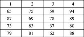
Consider a situation, where four groups of students were randomly assigned to be taught with four different techniques, and their achievement test scores were recorded (Table 8.7). Are the distributions of test scores the same, or do they differ?
Table 8.7 Database of four students and their scores
Step 1:
Rank all of the scores, ignoring which group they belong to. The procedure for ranking is as follows: the lowest score gets the lowest rank. If two or more scores are the same, then they are “tied”. “Tied” scores get the average of the ranks that they would have obtained, if they had not been tied. Here is the scores again, now with their ranks in brackets (Table 8.8)
Table 8.8 Database with rank
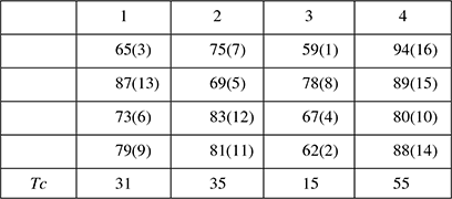
Find “Tc”, the total of the ranks for each group. Just add together all of the ranks for each group in turn.
Step 2:
Calculate the test statistics H, using the formula,
where N is the total number of participants, Ti is the rank total for each group. Thus in our problem,

Step 3:
The degrees of freedom is the number of groups minus one. In this problem, we have four groups, and so we have three degrees of freedom. Assessing the significance of H depends on the number of participants and the number of groups. Now we use the table of chi-square value to find significance of H. From the table, we have the rejection region described as, a right-tailed chi-square test with a = 0.05 and df = 4 − 1 = 3, reject H0 if H ≥ 7.81. Thus, we get the conclusion like, there is sufficient evidence to indicate that there is a difference in test scores for the four teaching techniques.
8.4.2 Steps for Kruskal-Wallis Test in SPSS
- Open the dataset in SPSS to be used for the Kruskal-Wallis test analysis.
- Click Analyze, click (mouse over) Non-parametric Tests, Legacy Dialogues and then click K Independent-Samples as shown in Fig. 8.5.
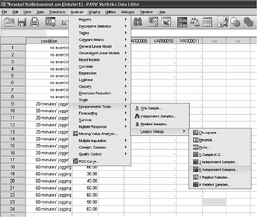
Fig. 8.5 Kruskal-Wallis in SPSS 1
Source: SPSS, Basev24, Statistical Package and Interface Package for SPSS, © 2014You should now be in the Test for Several Independent Samples dialogue box Click on the (Test Variable), and click arrow to move it to the Test Variable List: box Click on the (Grouping Variable), and click arrow to move it to the Grouping Variable: box Click Define Range and continue Click options under statistics and select Descriptive, click continue (Fig. 8.6).
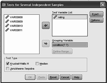
Fig. 8.6 Kruskal-Wallis in SPSS 2
Source: SPSS, Basev24, Statistical Package and Interface Package for SPSS, © 2014 - Make sure that Kruskal-Wallis H is checked in the Test Type area. Click Ok, and now it is ready to analyze the output.
A large amount of resources is required to compute exact probabilities for the Kruskal-Wallis test. Existing software only provides exact probabilities for sample sizes less than about 30 participants. These software programs rely on asymptotic approximation for larger sample sizes.
8.5 CHI-SQUARE TEST
A chi-squared test is a statistical hypothesis test in which the sampling distribution of the test statistic is a chi-squared distribution when the null hypothesis is true. The chi-square is used to test hypotheses about the distribution of observations into categories. The null hypothesis (H0) is that the observed frequencies are the same (except for chance variation) as the expected frequencies. If the frequencies observed are different from expected frequencies, the value of chi-square goes up. If the observed and expected frequencies are exactly the same, then chi-square equals zero ( χ2 = 0).
In chi-square test, we test whether a given χ is statistically significant by testing it against a table of chi-square distributions, according to the number of degrees of freedom for our sample.
Conducting chi-square analysis
- Make a hypothesis based on your basic question
- Determine the expected frequencies
- Create a table with observed frequencies, expected frequencies and chi-square values using the formula:

- Find the degrees of freedom
- Find the chi-square statistic in the chi-square distribution table
- If chi-square statistic ≥ calculated chi-square value, do not reject the null hypothesis and vice versa
Assumptions
The chi-square test for independence, also called Pearson’s chi-square test or the chi-square test of association, is used to discover if there is a relationship between two categorical variables. When we choose to analyze the data using a chi-square test for independence, we need to make sure that the data we want to analyze “passes” two assumptions.
- The two variables should be measured at an ordinal or nominal level (i.e., categorical data).
- The two variables should consist of two or more categorical, independent groups. Examples of independent variables that meet this criterion include gender (2 groups: Males and Females), profession (5 groups: surgeon, doctor, nurse, dentist, therapist) and so on.
8.5.1 Test Procedure
The test procedure consists of four steps: (1) state the hypotheses, (2) formulate an analysis plan, (3) analysis of sample data and (4) interpret results.
Stating the hypothesis
Suppose, variable A has r levels, and variable B has c levels. The null hypothesis states that knowing the level of variable A does not help predict the level of variable B. That is, the variables are independent.
Analysis plan
The analysis plan describes how to use sample data to accept or reject the null hypothesis. The plan should specify significance level and test method.
Analyze sample data
Using sample data, find the degrees of freedom, expected frequencies, test statistic and the P-value associated with the test statistic.
Expected frequencies: The expected frequency counts are computed separately for each level of one categorical variable at each level of the other categorical variable. Compute r * c expected frequencies, according to the following formula, ![]() where Er,n is the expected frequency count for level r of variable A and level c of variable B, nr is the total number of Z sample observations at level r of variable A, nc is the total number of sample observations at level c of variable B, and n is the total sample size.
where Er,n is the expected frequency count for level r of variable A and level c of variable B, nr is the total number of Z sample observations at level r of variable A, nc is the total number of sample observations at level c of variable B, and n is the total sample size.
Test statistic: The test statistic is a chi-square random variable (χ2) defined by the following equation, ![]() where Or is the observed frequency and Er is the expected frequency.
where Or is the observed frequency and Er is the expected frequency.
P-value: The P-value is the probability of observing a sample statistic as extreme as the test statistic. Since the test statistic is a chi-square, use the Chi-Square Distribution Calculator to assess the probability associated with the test statistic.
Interpret results
If the sample findings are unlikely, given the null hypothesis, we reject the null hypothesis. Typically, this involves comparing the P-value to the significance level, and rejecting the null hypothesis when the P-value is less than the significance level.
8.5.2 Chi-Square Test Procedure in SPSS Statistics
Step 1:
Click Analyze > Descriptive Statistics > Cross-tabs … on the top menu, as shown in Fig. 8.7.

Fig. 8.7 Chi-square in SPSS
Now a cross-tab dialogue box appears, transfer one of the variables into the Row(s): box and the other variable into the Column(s): box (Fig. 8.8).
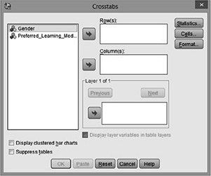
Fig. 8.8 Chi-square in SPSS
Step 2:
Now click on the SPSS Statistics button. It will be presented with the following Crosstabs: Statistics dialogue box (Fig. 8.9):

Fig. 8.9 Chi-square in SPSS
Select the chi-square and click continue.
Step 3:
Click the SPSS Cells button. It will be presented with the following Crosstabs Cell Display dialogue box. Select Observed from the Counts area, and Row, Column and Total from the Percentages area, as shown in Fig. 8.10 and then click the SPSS Continue button. This leads to generate the output (Fig. 8.10).

8.5.3 Example – Chi-Square Test
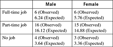
Consider the example of type of job (full time, part time, no job) that male and female does. Table 8.9 shows the initial record.
Table 8.9 Chi-square example database

Step 1:
Add numbers across columns and rows and calculate total number in chart. Now calculate expected numbers for each individual cell. For example, using the first cell in Table 8.9, we get the expected number as,
Step 2:
Now modify the table by entering the expected and observed values (Table 8.10).
Step 3:
Now calculate chi-square using the following formula,
So, for cell 1, we have,
Continue doing this for the rest of the cells, and add the final numbers for each cell together for the final chi-square number (final number = 0.0952). Now, calculate the degree of freedom,
Step 4:
At 0.05 significance level, with 2 df, the number in the lookup chart of chi-square test should be 5.99. Therefore, in order to reject the null hypothesis, the final answer to the chi-square must be greater or equal to 5.99. The chi-square/final answer found was 0.0952. This number is less than 5.99, so you fail to reject the null hypothesis.
8.6 MULTI-VARIATE ANALYSIS
Multivariate Analysis (MVA) is based on the statistical principle of multivariate statistics, which involves observation and analysis of more than one statistical outcome variable at a time. In design and analysis, the technique is used to perform trade studies across multiple dimensions while taking into account the effects of all variables on the responses of interest. Uses for multivariate analysis include the following:
- Design for capability (also known as capability-based design)
- Inverse design, where any variable can be treated as an independent variable
- Analysis of Alternatives (AoA), the selection of concepts to fulfill a customer’s need
- Analysis of concepts with respect to changing scenarios
- Identification of critical design drivers and correlations across hierarchical levels
The one-way multivariate analysis of variance (one-way MANOVA) is used to determine whether there are any differences between independent groups on more than one continuous dependent variable. In this regard, it differs from a one-way ANOVA, which only measures one dependent variable.
Assumptions while working with multivariate ANOVA
When you choose to analyze your data using a one-way MANOVA, part of the process involves checking to make sure that the data you want to analyze can actually be analyzed using a one-way MANOVA. You need to do this because it is only appropriate to use a one-way MANOVA if your data “passes” six assumptions that are required for a one-way MANOVA to give you a valid result.
- Two or more dependent variables should be measured at the interval or ratio level (i.e., they are continuous).
- Independent variable should consist of two or more categorical, independent groups.
- It should have an independence of observations, which means that there is no relationship between the observations in each group or between the groups themselves.
- It should have an adequate sample size. Although the larger the sample size, the better for MANOVA. MANOVA needs to have more cases in each group than the number of dependent variables.
- There should be no univariate or multivariate outliers.
- It is required to have a linear relationship between each pair of dependent variables for each group of the independent variable. If the variables are not linearly related, the power of the test is reduced.
8.6.1 Test Procedure in SPSS-MANOVA
Step 1:
Click Analyze > General Linear Model > Multivariate … on the top menu as shown in Fig. 8.11.
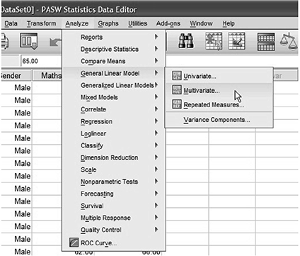
Fig. 8.11 MANOVA in SPSS
It will be presented with the Multivariate dialogue box, transfer the independent variable into the Fixed Factor(s) box and transfer the dependent variables into the Dependent Variables box. We can do this by drag-and-dropping the variables into their respective boxes or by using the SPSS Right Arrow Button.

Click on the SPSS Plots button. We can present the Multivariate: Profile Plots dialogue box. It helps in adding factors to axis and plots. While clicking the continue button, it comes back to the Multivariate dialogue box.
Step 2:
Click the SPSS Post-Hoc button. It will be presented with the Multivariate: Post Hoc Multiple Comparisons for Observed dialogue box, as shown in Figs. 8.13 and 8.14.
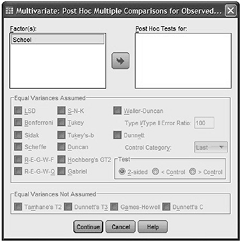
Fig. 8.13 MANOVA in SPSS
Transfer the independent variables, in to the Post Hoc Tests for: box and select the Tukey checkbox in the Equal Variances Assumed area. Click the SPSS Continue button and go to options. This will present you with the Multivariate: Options dialogue box, as shown in Fig. 8.14.
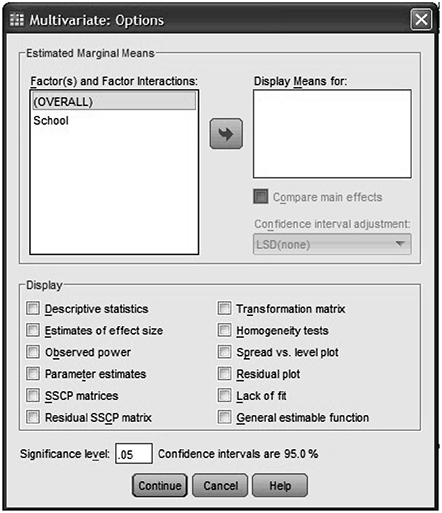
Fig. 8.14 MANOVA in SPSS
Transfer the independent variables, from the Factor(s) and Factor Interactions box into the Display Means for box. Select the Descriptive statistics, Estimates of effect size and Observed power check boxes in the Display area. Click the continue button and select OK. This will lead you to generate output.
EXERCISES
- The pupils at a high school come from three different primary schools. The head teacher wanted to know whether there were academic differences between the pupils from the three different primary schools. As such, she randomly selected 20 pupils from School A, 20 pupils from School B and 20 pupils from School C, and measured their academic performance as assessed by the marks they received for their end-of-year English and Maths exams. Therefore, the two dependent variables were “English score” and “Maths score”, whilst the independent variable was “School”, which consisted of three categories: “School A”, “School B” and “School C”. Which test procedure will be used and why? Also find the validity of the null hypothesis.
- Define and differentiate parametric and non-parametric test.
- Explain, analysis of variance.
- How one-way ANOVA differs from two-way ANOVA?
- What are the basic requirements for conducting Mann-Whitney test?
- In detail, explain the various assumptions that need to be taken care while conducting Kruskal-Wallis test.
- Define the step by step procedure for carrying out Chi-Square test.
- In detail, explain the various assumptions that need to be taken care while conducting Chi-Square test.
- Explain multivariate analysis.
- How is MANOVA different from ANOVA?
- When should a researcher adopt parametric test method?
- In detail, explain the various assumptions that need to be taken care while conducting ANOVA.
- Explain residual error.
- Use an appropriate non-parametric procedure to test the null hypothesis that the following sample of size n = 5 has been drawn from a normal distribution having mean as 100 and standard deviation as 10. Use α = 0.05.
93 97 102 103 105
- For analysis nominal data, which non-parametric statistics will you use? Why?