
Touro currently works part-time for the travel agency Tourista. His boss wanted him to estimate how demand for nondurable goods and services, from the population in general and from tourists in particular, would be affected by an increase in minimum wage in the state. Thus, he can’t wait to start this chapter, knowing that once he finishes with it, he will be able to:
1. Develop econometric models for simple linear regression;
2. Distinguish between the regression estimators and the estimates;
3. Analyze basic concepts for t-tests and goodness-of-fit measurements;
4. Perform data analyses and interpret the results using Excel.
Econometric Models
Prof. Metric reminds us that an econometric model is used to estimate the possible effect of an explanatory variable on a dependent variable. Chapter 1 has the following econometric model:
![]()
where SPEND is the spending on nondurable goods and services of a representative consumer, and WAGE his or her average weekly wage. The parameter a1 is the intercept and a2 the slope of the regression line. The random error e accounts for a set of unobserved factors (other than WAGE or any random component in the model) that might affect SPEND.
A general model for any variables is written as:
![]()
Since e captures the random component of y, we have the following equation for the regression line:
![]()
Booka raises her hand and asks, “Can anyone explain the notation E(y|x)?” Invo offers an explanation as follows:
E(y|x) is called the expectation of y given x. In Chapter 1, we learned to find E(X), which is expectation of X given several values of X such as x1, x2,…, xn. In this chapter, I think we are learning a new concept E(y|x), which implies that expectation of y is dependent on x instead of on several values of itself such as y1, y2,…, yn. For this reason, I believe that E(y|x), which is also written as E(y|x = xi), is classified as a conditional expectation and the whole function is called the conditional expectation function.
Prof. Metric commends Invo on his correct observation and points out that the error term e is the difference between actual y and its mean, as deduced from equations (2.2) and (2.3):
e = y − E(y|x) = y − (a1 + a2 x).
This error term also captures any estimation error that arises and any random behavior that might present in each individual identity.
Prof. Metric says that we will consider two types of data in this section: cross sectional and time series. A cross-sectional dataset presents many identities, which can be individuals, cities, states, and so on, in a single period. A time-series dataset tracks a single identity over many periods, which can be days, weeks, months, years, and so forth. Regarding cross-sectional data, the subscript i refers to the entity being observed, and the six classic assumptions are:
(i) The model is given by a linear function
yi = a1 + a2 xi + ei.
(ii) E(ei) = E (yi) = 0.
(iv) Cov(ei, ej) = Cov(yi, yj) = 0 for i ≠ j.
(v) xi is not random and must take at least two different values.
(vi) ei ~ N(0, σ2); yi ~ ([a1 + a2 xi], σ2).
For time-series data, assumption (v) changes to:
(v) yt and xt are stationary random variables and must take at least two different values, and et is independent of current, past, and future values of xt.
The remaining assumptions for cross-sectional data hold for time-series data, except that in this textbook the subscript i is changed to t and the subscript j is changed to z.
Regarding the stationarity in assumption (v) for time-series data, Prof. Metric says that we can roughly think of a stationary series as one that is neither explosive nor wandering aimlessly and that we will discuss this concept in detail in the later chapters. We also learn that data with the constant variance for all samples are said to be homoskedastic, and data with different variances for different samples are said to be heteroscedastic, which will be discussed in Chapter 4.
Simple linear regression often uses the least squares technique, also called ordinary least squares (OLS), because this technique minimizes the sum of the squared differences between the observed values of y and their expected values E(y|x). If assumptions (i) through (v) hold, then the Gauss-Markov theorem states that the OLS estimator will produce the best linear unbiased estimators (BLUE). If assumption (vi) also holds true, in addition to the other five assumptions, then the test results are valid.
The Central Limit Theorem (CLT) is very convenient for the assumption (vi). The theorem states that given a sufficiently large sample size from a population with a finite level of variance, the mean of all samples from the same population will be close to the mean of the population. In addition, all variances will be close to the variance of the population divided by each sample’s size. In this case, the test results are valid.
Taila then asks, “What do they mean by sufficiently large?” Prof. Metric commends her on the question and says that the question of “how large is large enough” is a matter of interpretation, but a cross-sectional sample with 30 data points or a time-series sample with 20 data points is usually considered large enough to cite CLT for valid test results.
Estimators and Estimates
Interpreting Coefficient Estimates
We learn that we need to collect data for estimations and that the estimated version of equation (2.2) is:
![]()
Prof. Metric says that the derivation of the OLS estimators in a simple linear regression needs knowledge of calculus and can be found in Verbeek (2012). We are only required to know that the estimators for the parameters â1 and â2 are written as:
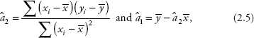
where ![]() is the sample mean of x, and
is the sample mean of x, and ![]() is that of y.
is that of y.
Specific values for â1 and â2 are called coefficient estimates (or estimates for short). Some econometricians also call them estimated coefficients. They are in fact point estimates, which provide a single value for each parameter of the OLS regression.
Once each parameter is estimated, the OLS estimates are interpreted according to the econometric model we develop. In general, the intercept â1 estimates the parameter a1, which measures the number of unit changes in y when x is zero, whereas the slope â2 estimates a2, which measures the number of unit changes in y due to a unit change in x.
For example, the intercept in equation (2.1) represents a person’s spending on nondurable goods when his or her wage is zero, whereas the slope represents the number of unit changes in spending due to a unit change in weekly wage. If wage is the only source of income for this representative consumer, then the slope measures the marginal propensity in nondurable spending.
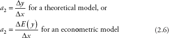
The slope of an OLS regression can be used to measure elasticity as well. Theoretically, the equation for elasticity is:
![]()
In econometrics, we can use the expressions in equation (2.6) to write the formula for calculating elasticity:
![]()
Hence, the estimation of elasticity is:
![]()
where the definitions of the variables are the same as those in the previous sections.
Prof. Metric says that there is a special case when both sides of equation (2.2) are in natural logarithmic form so that we have data for percentage change of y and percentage change of x. In this case, we do not have to follow equation (2.7), because â2 itself will measure percentage change of y due to one percent change of x, which is the elasticity.
Point Estimates
We learn that equation (2.5) can be used to calculate the point estimates of the OLS regression. Since all econometric software provide point estimates, Prof. Metric refers us to Table 2.1 at the end of the chapter, so that we can follow the steps provided in this table to practice calculating those point estimates of â1 and â2.
Suppose that substituting all variables into equation (2.5) yields â2 = 0.5 and â1 = 1.5, then the equation for the regression line becomes:
ŷi = 1.5 + 0.5 xi,
where 1.5 is the intercept and 0.5 is the slope of the line.
Invo exclaims, “Oh, if we let y be weekly spending and x weekly wage, both in hundreds of dollars, then the results imply that
(i) Weekly spending of a person without wage is $150 (= 1.5*$100), and
(ii) A $100 increase in weekly wage raises spending by $50 (= 0.5*$100).”
Prof. Metic commends Invo for his correct answers and moves to the next topic.
Interval Estimates
Prof. Metric says that in the previous subsection we only learned how to calculate point estimates. These point estimates do not account for any uncertainty in everyday life. Hence, we need to learn how to calculate an interval estimate, which provides a range of values instead of one single value for each parameter. This will allow us to face any uncertainty and still be able to state with a certain level of confidence that the actual value will likely fall between the upper and lower bounds (also called the endpoints) of this range.
To calculate interval estimates, a t-distribution for a sample of N observations is given as:
![]()
where N−2 = the degrees of freedom (df ) for the simple linear regression,
ak = the parameters to be estimated,
âk = the coefficient estimate from the OLS regression, and
se(âk) = the standard error of the coefficient estimate.
We learned earlier that if the classic assumptions (i) through (vi) hold, then the OLS estimators a1 and a2 have normal distribution. The same is true for â1 and â2.
![]()
where ![]()
Prof. Metric reminds us of a statistics concept, in which a standardized normal random variable Z is obtained as follows:
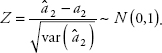
A similar formula can be written for a1. Given a critical value of Z (Zc)—for instance, α is the probability that the value is in the tail of the distribution—then the interval estimator is:
![]()
The CLT allows us to use the estimated values for the t-distribution as a substitution for Z when a sample is large enough. In that case, a t-critical value from the t-distribution is given so that
![]()
Equation (2.9) provides an interval estimator of ak. The interval is expressed as a 100(1 − α)% confidence interval. For example, if we choose α = 0.01, then the confidence interval is 99 percent—that is, we are 99 percent confident that the actual value falls somewhere between the lower bound and the upper bound of the interval estimate.
Prof. Metric says that we can choose a 90 percent confidence interval (α = 0.10) or a 95 percent confidence interval (α = 0.05) or a 99 percent confidence interval (α = 0.01). Most of the time, we choose the middle value (α = 0.05). Note that the interval has an upper bound and a lower bound. Hence, we will have to divide α into two tails, α/2 = 0.025, so that the total value of α is 0.05 (α = 0.025 + 0.025 = 0.05) and the confidence interval is 95 percent.
He then gives us an example: Suppose the sample size is N = 32 (df = 30), â2 = 0.5, and se (â2) = 0.1. Choosing a 95 percent confidence interval so that α = 0.05, we calculate the interval as follows.
On each of the two tails, α/2 = 0.025. We then look at a t-table for a critical value and find that tC = t(0.975, 30) = 2.042. Taila tells us that we can also type =TINV(0.05, 30) into any Excel cell to obtain tC = t(0.975, 30) = 2.042. We are very impressed with her intelligence. We find that the interval estimate for a2 is:
0.5 ± 2.042*0.1 = 0.5 ± 0.2042 = (0.2958; 0.7042).
Touro exclaims, “Oh, then we are 95% confident that a $100 increase in weekly wage will raise nondurable spending anywhere from $29.58 to $70.42, depending on, I guess, the individual characteristics.” Prof. Metric praises Touro for the correct interpretation and guides us to the next topic.
Estimating Var(ei)
Invo recalls equation (1.6) for variance and volunteers to write:
![]()
We are wondering why the second term in the formula disappears. Invo explains, “Assumption (ii) tells us that E(ei) = E (yi) = 0.” We now realize that what he says is true and guess that we can take the average of the squared errors as an estimator of σ2, which is written as:
![]()
It turns out that this formula does not help, because the errors ei are unknown. Prof. Metric tells us to recall the error term in equation (2.3) and the analog of it—namely, the OLS residual in equation (2.4). We are able to derive the following expressions from these two equations:
ei = yi − (a1 + a2 xi),
êi = yi − (â1 + â2 xi).
Since their error terms are similar, we guess that we can use the regression residual êi in place of the errors ei:
![]()
Touro says that this formula seems to have the same problem as the one in equation (1.7). Prof. Metric says that Touro is correct and refers us to equation (1.8) so that we can write an unbiased estimator of σ2 as:
![]()
Taila exclaims, “Wow, we must have learned to estimate all parameters in this simple linear regression model.” Prof. Metric smiles and says, “No, we have one more parameter to estimate: the predicted value of y, and equation (2.11) will be helpful for the interval prediction of y.”
Predicted Value
We learn that once coefficient estimates are obtained, the value of y, called the predicted value, can be calculated by substituting these parameters into the model. From Table 2.1, the prediction for y when x = 6 (that is, $600) can be calculated using equation (2.4) as follows:
ŷ = 1.5 + 0.5*6 = 1.5 + 3 = 4.5 ($ hundreds) = $450.
Thus, a person with a weekly wage of $600 will spend $450 on nondurable goods and services.
Prof. Metric says that interval prediction can also be calculated in a similar manner using the standard error of the prediction se(p) for the model. Let ŷ1 = â1 + â2 x1, then a formula in Kmenta (1997) can be used for calculating an approximation of the se(p):
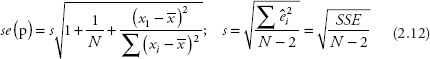
where s = the standard error of the regression, which is the square root of s2 in equation (2.11) and
SSE = the sum of the squared errors, which are often called the residuals in regression.
The interval prediction is calculated by replacing se(âk) in equation (2.9) with se(p):
![]()
Prof. Metric then tells us to use the aforementioned point estimate of $450 for weekly spending and calculate an interval prediction. He gives us se(p) = 0.5, N = 32, and α = 0.05. We are able to look at a t-table for a critical value and find that tC = t(0.975, 30) = 2.042, so the two endpoints of the interval prediction for weekly spending are:
4.5 ± 2.042*0.5 = (3.479; 5.521).
Hence, we predict with 95 percent confidence that a person with a weekly wage of $600 will spend anywhere from $347.90 (the lower bound) to $552.10 (the upper bound) every week.
Hypothesis Testing
Prof. Metric says that t-tests are used to verify the statistical significance or the expected values of the regression coefficients. Since simple linear regression has only one independent variable, the t-test for the significance of â2 also serves as the test for model significance.
Four Standard Steps
A t-test is usually carried out in four standard steps, shown as follows:
(i) State the hypotheses.
Define a constant c as a specific value for a parameter that we want to test.
If the null Ho is ak ≤ c, then the alternative Ha is ak > c.
If the null Ho is ak ≥ c, then the alternative Ha is ak < c.
If the null Ho is ak = c, then the alternative Ha could be ak > c or ak < c or ak ≠ c.
(ii) The test statistic:
![]()
where k = 1 or 2 in a simple regression. (2.14)
(iii) The critical t-value, tC, which indicated the border point of the rejection region, depends on the significance level of the test, which is usually at 1%, 3%, or 10%.
(iv) Decision: If |tSTAT| ≥ tC, we reject the null and follow the alternative hypothesis. Otherwise, we do not reject the null. We then draw the meaning and the implication of our decision concerning the parameters of a regression.
We learn that there are two basic types of t-tests: If c is any constant other than zero, we have a test of a general hypothesis; and if c is zero, we have a test of significance, because a parameter only has a significant impact on a model if it is not zero. Prof. Metric emphasizes to us that the tails of the tests always follow the alternative hypotheses. There are only three cases: in the alternative hypothesis (Ha), if ak > c, we have a right-tailed test; if ak < c, we have a left-tailed test; and if ak ≠ c, we have a two-tailed test.
Tests of the General Hypothesis
Booka offers an example. Last week she wanted to find out the demand for books in relation to income. The dependent variable is spending on books (BOOK), and the independent variable is per capita income (PERCA). She found the following relationship between the two variables: BOOK = 0.09*PERCA, and se(â2) = 0.015. Booka says that she conducted a survey of 34 customers, so N = 34. We proceed to perform several tests as follows:
Invo says, “Let’s test the alternative hypothesis a2 > 0.06 against the null hypothesis a2 ≤ 0.06.” We agree with him and perform the test as follows:
(i) H0: a2 ≤ 0.06; Ha: a2 > 0.06.
(ii) tSTAT = t(N−2) = (0.09 − 0.06)/0.015 = 2.
(iii) We decide to choose α = 0.05, so tC = t(0.95, 32) = 1.694.
Prof. Metric says that Excel always reports a two-tailed critical value, so to find t-critical for a one-tailed test, type =TINV(2α, df) into any cell, then press Enter.
For example, typing =TINV(0.10, 32) into any empty cell and then pressing the Enter key yields the result of 1.6939 ≈ 1.694.
(iv) Decision: Since |tSTAT| > tC, we reject the null (H0), meaning a2 > 0.06, thus implying that the customers of the bookshop tend to spend more than 6 percent of the increase in their income on books.
A left-tailed test
Touro wants us to test the alternative hypothesis a2 < 0.15 against the null hypothesis a2 ≥ 0.15. We proceed with the test as follows:
(i) H0: a2 ≥ 0.15; Ha: a2 < 0.15.
(ii) tSTAT = t(N−2) = (0.09 − 0.15)/0.015 = −4.
(iii) We try α = 0.01 this time, so tC = t(99, 32) = 2. 449 (or (−tC) = −2. 449). We also type =TINV(0.02, 32) into Excel, which gives us 2.44868 ≈ 2.449.
(iv) Decision: Since |tSTAT| > tC (or tSTAT < (−tC)), we reject the null (H0), meaning a2 < 0.15 and implying that the customers tend to spend less than 15 percent of the increase in their income on books.
Tests of Significance
A one-tailed test
Prof. Metric wants us to test the significance of the slope, so the null hypothesis states that the slope is zero. Since the right-tailed test and the left-tailed test are very similar, we choose to test the alternative hypothesis for a2 > 0:
(i) H0: a2 = 0; Ha: a2 > 0.
(ii) tSTAT = t(N−2) = (0.09 − 0)/0.015 = 0.09/0.015 = 6.
(iii) We decide to choose α = 0.01 again, so tC = t(0.99, 32) = 2.449.
(iv) Decision: Since |t(N−2)| > tC = t(0.99, 32), we reject the null, meaning a2 > 0 and implying that income has a positive effect on book spending.
A two-tailed test
This time, Booka wants to test the alternative a2 ≠ 0. Prof. Metric agrees and says that the left-tailed test of significance is similar to the right-tailed test, so we do not have to try it in the class. We now perform the two-tailed test as follows.
(i) H0: a2 = 0; H1: a2 ≠ 0.
(ii) tSTAT = t(N−2) = (0.09 − 0)/0.015 = 0.09/0.015 = 6.
(iii) Since this is a two-tailed test, Prof. Metric reminds us to use α/2 = 0.025, and so
tC = t(0.975, 32) = 2.037.
For a two-tailed test, we learn to type =TINV(α, df) into any cell in Excel.
So, we type =TINV(0.05, 32), then press Enter. Excel gives us 2.0369 ≈ 2.037.
(iv) Decision: Since |tSTAT| > tC, we again reject the null, meaning a2 ≠ 0 and implying that income does have a significant impact on book spending. We also recall the earlier discussion and are able to state that the model is statistically significant as well.
Prof. Metric reminds us that Excel reports the tSTAT value for the two-tailed test of significance—that is, in the null hypothesis (H0) ak = 0 and in the alternative hypothesis (Ha) ak ≠ 0. This tSTAT is also called the t-ratio because we only need to divide ak by se(ak) when c = 0. You will hear about this t-ratio from a lot of researchers because it is one of the most important statistics in econometric study.
Goodness-of-Fit and P-Value
Taila asks, “How can I compare two models and find out exactly which one predicts better?” Prof. Metric says enthusiastically that it is quite possible to do this, and that it is called ”goodness-of-fit.” We will learn about goodness-of-fit in this section.
R-squared (R2)
We learn that an R2 value can measure how much the variation in y can be explained by the variation in x. In the first section, we have the estimated equation as:
![]()
Subtracting the sample mean from both sides of this equation gives us:
![]()
Square both sides of the previous equation and take the sum of these expressions to obtain:
![]()
We know that the cross term ![]() is zero because E (ȇ) = 0, so
is zero because E (ȇ) = 0, so
![]()
The following definitions are commonly used for the squared terms in equation (2.15).
![]() = the total sum of squares (SST)
= the total sum of squares (SST)
![]() = the sum of squares of the regression (SSR)
= the sum of squares of the regression (SSR)
![]() = the sum of squared errors (SSE).
= the sum of squared errors (SSE).
Given these definitions, the R2 value is the coefficient of determination and is defined as
![]()
If R2 = 1, the model is said to have a perfect fit. In practice, we always find that 0 < R2 < 1. R2 is reported by all econometric packages, including Excel. If R2 is high, then the model is a good fit; for example, R2 = 0.92 implies that 92 percent of the variation in the dependent variable can be explained by the independent variable. If R2 is low, then the model is not a good fit.
Prof. Metric points out that in Figure 2.2 of the Data Analyses section, SSR, SSE, and SST are reported in cells H12, H13, and H14, respectively.
P-Value
We learn that p-values can be used to measure the exact significance level of the aforementioned estimates. A p-value indicates the probability that a random variable falls into the rejection region at a particular significance level. Invo exclaims, “Sounds too abstract for me to understand. Can anyone explain more clearly what p-values really measure?”
Taila offers an explanation,
When we run a regression, the null hypothesis is the possibility that there is no effect on our results. For example, an experiment for a medical treatment that we know is totally ineffective. The null hypothesis is true: there is no difference between the experimental groups at the population level. Despite the null being true, it is possible that there will be an effect in the sample data due to random sampling error. P-values measure how well the sample data support the argument that this medical treatment has no effect. A high p-value implies our data are likely with a true null, and a low p-value implies our data are not likely with a true null. In the above example, a low p-value suggests that your sample provides enough evidence for you to reject the null of no effect in the medical treatment.
Prof. Metric praises Taila and provides us a numerical example: A p-value = 0.002 for a model implies that we reject the null at a 0.2 percent significance level, which is a very good fit because we need the model to satisfy only 5 percent significance level. A formula for calculating p-values is introduced in Hill et al. (2011), but most econometric packages, including Excel, report p-values, so we do not have to learn this skill.
Thanks to this practice, we can look up p-values instead of going through the steps of calculating tSTAT and depending on the t-table for t-critical values. We can always reject the null hypothesis if the p-value ≤ α, where α could be 0.01, 0.05, or 0.10. For example, if we choose α = 0.05, then we reject the null if the p-value ≤ 0.05. The following values are generally used for the tests of coefficient significances:
If p-value ≤ 0.01: the coefficient estimate is highly significant.
If 0.01 < p-value ≤ 0.05: the coefficient estimate is significant.
If 0.05 < p-value ≤ 0.10: the coefficient estimate is weakly significant.
If p-value > 0.10: the coefficient estimate is not statistically significant.
Prof. Metric asks us to look at Figure 2.2 in the Data Analyses section in order to practice how to interpret p-values: From this figure, the coefficient estimate of the intercept is reported in cell J17 and it is only weakly significant (with p-value = 0.065); whereas, the slope estimate is reported in cell J18 and it is highly significant (with p-value = 1.398*10−29). Invo exclaims, “I see another value of 1.398*10−29 reported in cell K12. Is that the p-value for the significance of the whole model?” Prof. Metric commends him on the remark and says that this is true.
Data Analyses
Performing a Regression
Prof. Empirie says that we usually have three types of data for performing regression: cross sectional, time series, and longitudinal/panel. We discussed cross-sectional and time-series data at the beginning of this chapter. A longitudinal/panel dataset follows many identities over many periods.
Prof. Empirie reminds us again that all data are available in the folder Data Analyses.
Invo has collected data on expenditure on durables (DUR) and personal income (INCOME) for 51 cities (ID) in 2015. He tells us that the dataset is too large to display but is available in the file Ch02.xls. Fig.2.1-2.2. We want to see if DUR depends on INCOME—that is, if DUR is the dependent variable and INCOME the independent variable. We open the data file and follow these steps to perform a regression of DUR on INCOME:
Select Data and then Data Analysis on the ribbon.
Click Regression in the list instead of Descriptive Statistics, then click OK.
A dialog box appears, as shown in Figure 2.1.
Type B1:B52 into the Input Y Range box.
Type C1:C52 into the Input X Range box.
Select the Labels and Residuals boxes.
Select the Output Range button and enter F1.
Click OK; you will see another dialog box stating that data will be overridden.
Click OK again to overwrite the data.
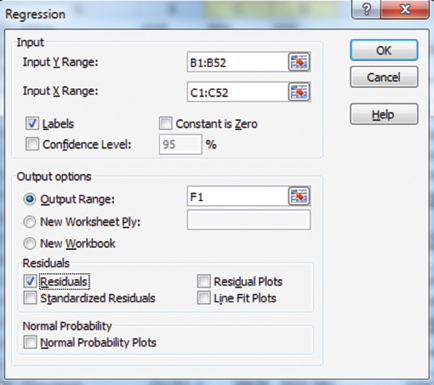
Figure 2.1 Performing regression: Commands in dialog box
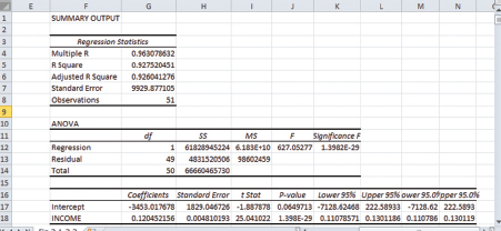
Figure 2.2 Simple linear regression results
The regression results are shown in Figure 2.2. Prof. Empirie then guides us to study Figure 2.2 and writes the estimated results (also called estimated equation) as follows:
DURi = −3453 + 0.1205 INCOMEi.
(se) (1829) (0.0048) R2 = 0.9275
To obtain the predicted value for DUR in 2016, we need to substitute any value of INCOME for a city into this equation. It turns out that when we click Residuals, Excel automatically calculates predicted values and reports them next to the residuals. For example, you can find the predicted DUR for the first city in cell G25 of the data file for Figure 2.2, which is 20,489.25.
Taila points out that she also found the upper and lower 95 percent bounds for the coefficient estimates in cells K17 through L18, which are repeated in cells M17 through N18. Prof. Empirie praises her for her keen observation and says that Excel does not report the interval estimates for the predicted values, so if we wish to know these values, we will have to calculate them using equations (2.7) and (2.8).
She then tells us that we will have opportunities to get hands-on experiences with time-series data and panel data in the later chapters.
1. Given the information in Table 2.1, perform the following procedures:
(a) Fill in the blank spaces and then use the information in this table to calculate â1 and â2.
(b) What is the interpretation of â1 and â2 if the dependent variable is yearly salary in ten thousands of dollars and the independent variable is college education in years?
2. Given the following estimation results:
DEMAND = 4.198 − 3.229 PRICE
(se) (1.012) (0.5017) R2 = 0.633 N = 26,
provide comments on the significances of a1 and the implication of the R2.
3. Use the results in Exercise 2 to test the following hypotheses at a 1 percent significance level:
(a) Test the slope is −3 against the alternative hypothesis that the slope is smaller than −3.
(b) Test the slope is zero against the alternative hypothesis that the slope is not zero.
Write the testing procedure in four standard steps similar to those in the text. The calculations of the t-statistics may be performed using a handheld calculator or using Excel.
Table 2.1 Information for calculating coefficient estimates
Variable |
x |
|
y |
|
|
|
|
3 |
|
4 |
|
|
|
|
2 |
|
2 |
|
|
|
|
1 |
|
3 |
|
|
|
|
|
|
|
|
|
|
Table 2.2 Information for calculating R2
y |
|
|
|
2 |
|
|
|
−1 |
|
|
|
2 |
|
|
|
|
|
|
|
4. Given the information in Table 2.2, fill in the blank spaces and then use the information in this table to calculate R2 if SSE = 0.60. Provide comments on the result.
5. Data on education expenditures (EDU) and per capita income (PERCA) for 50 states and Washington, DC, in 2014 are in the file Education.xls.
(a) Perform a regression of PERCA on EDU (dependent variable = y = PERCA; independent variable = x = EDU), write the estimated equation, and find the point predictions for PERCA.
(b) Provide comments on the coefficient estimates and R2.