Chapter 9. Communicating Your Design in Excel
▪ Communicate your design, including design specifications
▪ Add a ScreenTip (tooltip) to a content hyperlink
▪ Insert comments
▪ Add annotation areas
Introduction
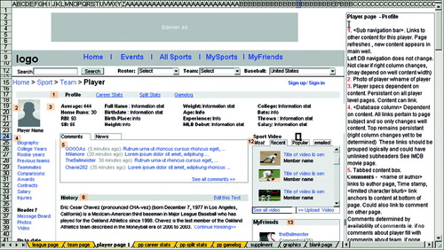
If a picture can represent a thousand words, a prototype can elicit a thousand and one interpretations. Now that you have created a prototype of your design, you'll want to narrow the number of interpretations. To that end, you can add accompanying communications to your prototype. Prototypes rarely speak for themselves, and even when they do, they generally never tell the complete design story. Without good communications, other stakeholders can neither understand your design intent nor understand its context. Good communication should indicate what still needs to be further fleshed out or documented in your prototype.
After completing a prototype version but before you pass it on to others, establish clear, logical design communications based on
▪ Design objectives and rationale
▪ Requirements on which you based your design and applied to your prototype
▪ Design guidelines and specifications
▪ Task and navigation flow mappings
▪ Priority screens
▪ Design decisions and issues in the form of annotations
These communications help you reflect which objectives you have or have not addressed in your prototype. They can also be used to set audience expectations regarding your prototype. Creating clear communications and setting expectations, in turn, will help to avoid many of the inevitable opinion battles that often arise when presenting and rationalizing your design. Likewise, documenting your design rationale helps you remember why you made certain design decisions and helps you communicate that rationale to others.
▪ Tooltips
▪ The built-in comment feature
▪ An annotation area within worksheets that contain your designs
▪ A separate worksheet devoted specifically to communicating your design
If you are creating a prototype for an internal group that already has a deep understanding of your design or if your changes are small in scope, you might need only minimal communications. On the other hand, if you are creating an entirely new interface or making significant changes to an existing design, you might want to choose a communication method that can support long and detailed descriptions of your ideas.
Table 9.1 will help you decide which of these communication techniques to use.
Adding a Tooltip to Excel Hyperlinks
As part of the hyperlinking function in Excel, you can add rollover tooltips (referred to as ScreenTips in Excel) to a hyperlink text or graphic. This method can be very helpful for including a succinct note about the hyperlink. However, there are a couple of drawbacks. First, you cannot add the notation to plain text—the text must be a hyperlink to have a ScreenTip. Second, there is no indication that the link includes a ScreenTip until you hover your cursor over the hyperlink text.
In some cases, you are prototyping an entire page with many hyperlinks; however, only a few hyperlinks have a tooltip. How can you tell the difference? You can also use your own variations on colors, underlining, bolding, and so on; just make sure your convention is adequately communicated to your audience.
In this exercise you will learn how to create tooltips in a prototype.
To Create a ScreenTip Annotation:
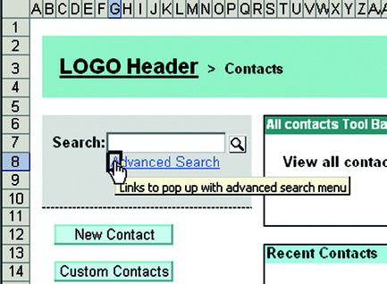
For example, you might want to create an annotation for the Advanced Search link, noting that this will be a pop-up link and not a link to another page. In this exercise and throughout this chapter you will continue using the same file you used in Chapter 8.
2 When the pop-up contextual menu appears, click Hyperlink (Figure 9.1).

3 The Insert Hyperlink dialog box offers choices of what you can link to. In this case, link to the Advanced Search worksheet that has already been prepared in your workbook. In the input box at the top of the dialog, add the text that describes where the Advanced Search link goes (Figure 9.2).

4 In the upper-right corner of the dialog, click the ScreenTip button, which opens a dialog box with a text box for your notation (Figure 9.3).

5 Click OK for the ScreenTip and the Insert Hyperlink windows. The Advanced Search text has become a link. When you roll over it, the annotation you have written appears (Figure 9.4, page 172).
For the tooltip to appear, you must roll over the first table cell that includes the hyperlink. If you want all the hyperlinked text to trigger the tooltip, you have to merge all the cells behind the hyperlink text.

All the cells behind the linked text will now display the text annotation on rollover (Figure 9.6).

Inserting Comments
Excel's commenting feature is an ideal way to make annotations on a specific area of a prototype that is not a hyperlink or graphical element. Excel's commenting is flexible to use and can be modified in many ways. By placing comments in table cells close to the features in your design, you can indicate what you are commenting on. The comments themselves can be modified by type, size, shape, color, or border style. The comment box can expand to accommodate relatively large amounts of text. Through the Reviewing toolbar, you can cycle through all your comments, show them all at once, or hide them.
A red triangle in the upper-right corner of the table cell indicates a comment on a cell. Be careful—many comments on a worksheet can distract from your design. Another consideration in including comments is that all your comments will be isolated boxes scattered across your design. Though this helps in visually linking what the comments describe, it can be difficult to read them all at once or to copy them all to another design or requirements document.
To illustrate comments, we will use a case study using a New Contacts button in a design. This button is a new feature and will need a lengthy explanation.
In this exercise you will learn how to insert comments, customize the comments area, and use the reviewing menu to display the comments.
To Insert a Comment:
1 Right-click the corner of the contact button cell and select Insert Comment (Figure 9.7).

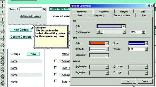
2 Right-click the red comment icon and the comment box opens. Here you can add text; in our example we added This button is under technical feasibility review by the engineering team (Figure 9.8).

4 To give the comment box the same style as all other technical comments in the prototype, in the Format Comment dialog box choose the Colors and Lines tab and give this comment box a blue background with an orange border (Figure 9.9, page 176).
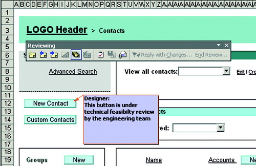
The end result will have the style attributes defined in the dialog box and will look like Figure 9.10 (page 176).

After making several comments on the worksheet, you can manage them by opening the Reviewing toolbar. Use this toolbar to cycle through all the comments you've made, open them all up, or hide them.
In the Reviewing toolbar (Figure 9.11, page 177), you can
▪ Edit Comment: To edit comment text
▪ Next Comment: To go from one comment to the next comment
▪ Show Comment/Hide Comment: To toggle the visibility of the comment in a selected cell
▪ Hide All Comments/Show All Comments: To toggle the visibility of all comments in a worksheet
▪ Delete Comments: To remove the comment from the currently selected cell
Creating Annotation Areas
You might want your annotations to appear on a worksheet without being hidden in a collapsible comment box or as hidden tooltip. By creating annotation areas, you can read the communications along with viewing the design.
First, you can make your own indicators, or graphical callout elements, that you position on the designs. These indicators act as references to your annotations.
▪ You can have all your annotations on a different worksheet within the workbook and link back and forth between the different worksheets.
▪ If your design is the full width of the application window, you can position a text box to enter your annotations off to one side so that they don't impose on your design and are either
▪ If you change the zoom to 75 percent, the annotations can be revealed and hidden by zooming back to 100 percent
▪ You can position the text box at the bottom of your design to keep annotations out of view. Making your indicators anchor links within the worksheet lets you link to the annotation for easy access.
▪ You can also link between Excel workbooks or other applications, such as Word. By using a word processing application, you can use more robust text tools to express your annotations if desired.
In this exercise you will learn how to annotate your prototype by creating areas on a worksheet with anchor links to annotations.
For this exercise we will create annotations in a separate worksheet. In anticipation of making annotations, you can create a series of indicators and place them in your image library worksheet in your Excel template. An indicator is an AutoShape with a numerical text reference.
To Create Annotation Areas:
1 From the Drawing toolbar, choose AutoShapes > Basic Shapes > Rectangle. Holding down the Shift key, create a small square.
2 Right-click the square and choose Format AutoShape. In the Format AutoShape dialog box, select an orange Fill Color, and set Fill Transparency to 50% (Figure 9.12). Click OK.

We click Transparency so that annotations will not obscure any graphics that they are placed on top of.
3 Right-click the orange square, choose Add Text, and enter the number 1.
4 Repeat steps 1–3 to make five square indicators (Figure 9.13).

5 Select the first indicator and copy it.
6 Go to the wireframe2 tab. Place the cursor above the groups box and paste the indicator (Figure 9.14, page 180).

7 Create a new worksheet and call it Annotations.
8 Use the rectangle AutoShapes tool, as you did in step 1, but this time click and drag a large area.
9 Add text: Annotation 1 (Figure 9.15, page 181).

10 Go to the Wireframe2 worksheet. Select the Indicator, right-click, and choose Hyperlink.
11 As you have in other procedures, choose Place in This Document and select annotation (Figure 9.16).

12 Click OK.
This will link the indicator to the annotation.
13 To create a link to return from the annotation back to the wireframe, go to the annotation worksheet.
14 Select cell 2J and enter the text <Back.
15 Select the cells behind the text <Back, right-click, and choose Hyperlink.
16 In the Insert Hyperlink dialog box, link back to the Wireframe worksheet (Figure 9.17, page 182).

17 Click OK.
18 Repeat this process to annotate all necessary elements.
Your image will look something like Figure 9.18 (page 183).

This is where you will enter your annotations. Because the team might miss the annotation area, make your annotation indicators anchor links to the annotation area.
20 In the Type the Cell Reference text box, enter the cell reference cc1, which is the upper-right cell above your Annotation box.
21 To make it easy for your team to navigate from the annotation box back to your design, create a Return link above the box by using the default coordinates that will return a viewer to the original page orientation (Figure 9.19, page 184).

The annotation box could be to the right of the design, below the design, on a different page in this workbook, or in a different workbook altogether (Figure 9.20, page 184).

Another way to organize your page annotations is to create a prototype that is smaller in width so that you can have space to the left or right of the design for your annotations and other documentation. In this example (Figure 9.21, page 185), the column widths are narrower than usual and the type font is set to 8 points so that the resulting page is approximately 75 percent of the size of a full-scale page. The advantage to this method is that all the annotations are within the width of a full page, allowing for direct visual access to the annotation without having to click to another position on the worksheet or hyperlink to another document.
Conclusion
With your prototype finished, the documentation you have created throughout the prototyping process can become part of your final specification document. If you are using an application such as Microsoft Word that has a hyperlink text feature, you can link to your prototype, and conversely you can link from the prototype to your specification document. Or you can use your Excel prototype as a combined specification and design communication document.
References
1. Jonathan, Arnowitz; Michael, Arent; Nevin, Berger, Effective Prototyping for Software Makers. (2007) Morgan Kaufmann, San Francisco.
2. Dan, Brown, Communicating Design: Developing Web Site Documentation for Design and Planning. (2006) New Riders Press, Berkeley.
..................Content has been hidden....................
You can't read the all page of ebook, please click here login for view all page.