A1.1. Cylindrical harmonics

Let R_c be the reference frame of cylindrical coordinates (r, θ, z) and center O. The Cartesian coordinates are then defined in terms of the cylindrical coordinates by the relations:

[A1.1]

Considering expression [A1.7] for the Laplacian in cylindrical coordinates given in Appendix 1 of Volume 1, the Helmholtz equation is written with M = L or T, depending on the type of wave:

[A1.2]

The solution to this equation is found using the separation of variables method:

[A1.3]

Substituting this trial solution into equation [A1.2] and dividing by RΘZ leads to:

[A1.4]

The third term is a function of the variable z only, while the rest depends on r and θ. It is necessarily equal to a constant (−k²), leading to equation:

[A1.5]

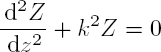
whose solutions are of the type:

[A1.6]

The same reasoning applied to the second term of equation [A1.4], which is written as:

[A1.7]

leads to the equation:

[A1.8]

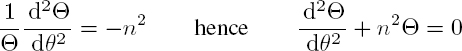
where n is a constant. The solutions of this equation are:

[A1.9]

Since the domain of study is defined for θ [0, 2π], n is necessarily an integer, so that the field is continuous at θ = 0 and at θ = 2π.

After the substitution, equation [A1.7] takes the form of the Bessel equation:

[A1.10]

whose general solution is:

[A1.11]

where J_n and Y_n are Bessel functions of the first and second kind, respectively. The solution R_n(k_⊥r) can also be expressed by:

[A1.12]

where are the Hankel functions defined by:

[A1.13]

The derivatives of the Bessel and Hankel functions verify the recurrence relations:

[A1.14]

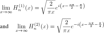
For x = 0, the function J₀ takes the value 1, while the other J_n functions are zero and the Y_n functions are all singular. The Hankel functions are also singular at the origin and have the specific feature that in the far field, they approach the functions:

[A1.15]

The potential is sought in the form of an expansion on the cylindrical harmonics:

[A1.16]

If the problem is independent of the z coordinate, the wave number k is zero and k_⊥ = k_M; the potential of the mode M is then expressed by:

[A1.17]

The developments of the exponential of a trigonometric function, given by Jacobi and Anger:

[A1.18]

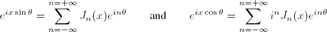
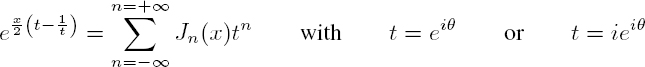
can be used, for example, to represent a phase-modulated wave or to convert a plane wave into a sum of cylindrical harmonics. These identities are deduced from the generating functions of the Bessel functions:

[A1.19]

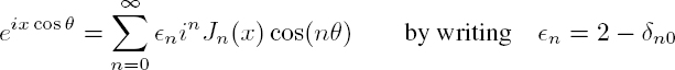
Since i⁻ⁿJ_−n(x) = iⁿJ_n(x), the second equation [A1.18] takes the form:

[A1.20]

A1.2. Spherical harmonics

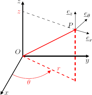
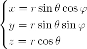
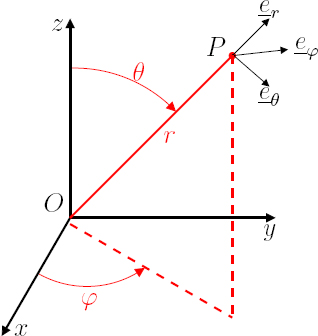
Let R_s be the reference frame of spherical coordinates (r, θ, ϕ) and center O. The Cartesian coordinates are then defined as a function of the spherical coordinates through the relations:

[A1.21]

Considering expression [A1.16] for the Laplacian in spherical coordinates, given in Appendix 1 of Volume 1, the Helmholtz equation is written in spherical coordinates as:

[A1.22]

The solutions are found using the separation of variables method:

[A1.23]

which, after dividing by RΘΦ, leads to the equation:

[A1.24]

Multiplying by r² sin² θ shows that the third term depends only on ϕ, while the rest depends on r and θ. Consequently, Φ satisfies the following equation:

[A1.25]

whose solutions are:

[A1.26]

to ensure continuity over the domain ϕ ∈ [0, 2π].

Considering this solution, equation [A1.24] takes the form:

[A1.27]

Multiplying by r² shows that the first and fourth terms depend only on r, while the second and third terms depend only on θ; equation [A1.27] can be divided into two parts¹:

[A1.28]

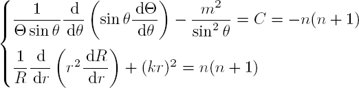
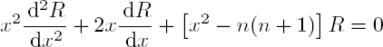
By changing the variable X = cos θ, the θ equation takes the form of an associated Legendre equation:

[A1.29]

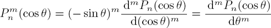
Its solutions are the Legendre functions of degree n and order m:

[A1.30]

which are derived from the Legendre polynomials of degree n (P_n) through a derivative of order m:

[A1.31]

If the problem is invariant with respect to the angle ϕ, m = 0 and the solution to equation [A1.29] is a Legendre polynomial of degree n: P_n(cos θ).

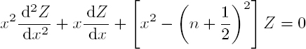
By performing the change in variable x = kr, equation [A1.28] in r is written as:

[A1.32]

The change in function leads to the Bessel equation [A1.10] for the index n + 1/2:

[A1.33]

Its solutions are Bessel functions of the first and second kind of fractional order:

[A1.34]

The R_n(kr) functions are thus expressed by:

[A1.35]

where the spherical Bessel functions of the first kind, j_n, and the second kind, y_n, are defined by:

[A1.36]

In some cases, it is preferable to introduce the spherical Hankel functions:

[A1.37]

to express the function R_n(kr):

[A1.38]

A1.2.1. Properties of spherical Bessel and Hankel functions

The derivatives of the spherical Bessel and Hankel functions satisfy recurrence relations identical to [A1.14]:

[A1.39]

At x = 0, the function j₀ takes the value 1, while the other functions, j_n, are zero and the y_n functions are singular. It follows that the Hankel functions are also singular at the origin and their asymptotic behavior in the far field:

[A1.40]

is that of a divergent wave for and a convergent wave for

A1.2.2. Properties of Legendre functions

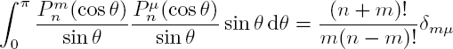
The associated Legendre functions verify the orthogonality relation:

[A1.41]

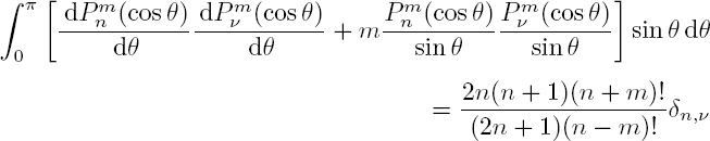
If m and μ are non-zero, they also verify the relation:

[A1.42]

Two other relations involving the Legendre functions are also useful:

[A1.43]

and

[A1.44]

A1.2.3. Expansion on spherical harmonics

Any scalar function that is a solution to the Helmholtz equation can be developed as an infinite sum of modes:

[A1.45]

called normalized spherical harmonics:

[A1.46]

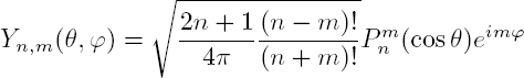
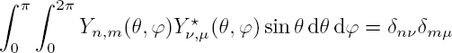
The amplitudes A_n,m of the spherical harmonics are deduced from the boundary conditions. The functions Y_n,m(θ, ϕ) are orthogonal and normalized functions; they verify the relation:

[A1.47]

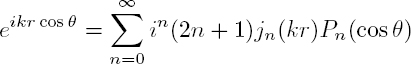
A development in spherical harmonics, very useful for acoustic scattering problems, is that of a plane wave propagating in the z direction:

[A1.48]