2
Scattering of Elastic Waves
In Volume 1, the propagation medium, assumed to be homogeneous, was either infinite (Chapter 1), divided into two parts by a plane interface (Chapters 2 and 3), or limited in one or two dimensions (Chapter 4), the waves propagating freely in this or other dimensions. Here, the propagation medium is locally inhomogeneous; these heterogeneities may be inherent to the structure or may result from manufacturing defects (inclusions) or from the aging of the parts (cracks). Waves scattered by an obstacle propagate away from it, possibly in privileged directions, even if the medium is isotropic. Several applications in underwater acoustics are based on target scattering: detecting mines or ships by an active sonar, locating shoals of fish, or mapping ocean floors. In non-destructive testing by ultrasound, the information carried by the scattered waves is used to characterize these heterogeneities or to prevent damage, such as the delamination of composite materials. Scatterers can be deliberately introduced, for instance, to attenuate backward waves emitted by a piezoelectric transducer and thus dampen its responses (section 3.1). Recently, the development of periodic structures (phononic crystals) or heterostructures made of resonant inclusions dispersed in a matrix (acoustic metamaterials) opened the way to the filtering and the control of elastic wave propagation.
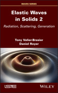
The interaction of a (plane) elastic wave with a particle embedded in a matrix gives rise to many phenomena (Figure 2.1), such as:
- – the reflection at the particle–matrix interface;
- – the transmission inside the particle with a possible mode conversion, and then internal reflections and refraction;
- – the conversion into waves propagating at the interface with the matrix, and then re-emission into bulk waves;
- – the diffraction by the edges of the object;
- – the absorption of part of the energy within the particle.
All of these phenomena, which can give rise to resonances involving bulk, surface or guided waves, have been studied separately in Volume 1. The scattering theory accounts for these phenomena in a global way. The approach consists of defining, in the harmonic case, an incident field and a scattered field that satisfy the propagation equations in each of the two media. The boundary conditions at the interface between the scatterer and the matrix are applied to the total field.
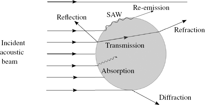
Figure 2.1. Interaction of an elastic wave with a scatterer. The incident energy is either reflected, or transmitted and then refracted, or converted into a surface acoustic wave (SAW) and then re-emitted, diffracted by the edges of the scatterer, or partially absorbed inside the scatterer
Formally, the displacement field u is written as the superposition of an incident displacement field ui and a scattered field ud, composed a priori of all the propagation modes M:
In a perfect fluid or an isotropic solid, the acoustic field associated with longitudinal waves is determined through the knowledge of a scalar potential Φ, while the field associated with transverse waves in the solid derives from a vector potential ψ. For obstacles having a canonical form (cylinder or sphere), the method of analysis consists of:
- – expanding the potentials of the incident wave on the basis of harmonic solutions (cylindrical or spherical) to the Helmholtz equation (see Appendix 1);
- – postulating a similar development, with unknown coefficients, for the scattered waves;
- – determining these scattering coefficients by applying, for both fields, the boundary conditions at the fluid–solid interface.
Due to the orthogonality of cylindrical and spherical harmonics, these conditions can be applied independently to each harmonic of order n. The problem can be reduced to the resolution of a linear system having, a priori, an infinite number of equations. Finally, the scattered field is obtained as an expansion of cylindrical or spherical harmonics. Fortunately, the number of terms can be reduced according to the convergence of the series of harmonic functions.
The interest in this model is to predict the evolution of the acoustic intensity scattered in each direction, according to the elastic and geometrical characteristics of the scatterer. The complexity of the calculation will quickly convince the reader of the advantage of considering the symmetry of the “incident wave + scatterer” configuration in order to reduce the number of modes to take into account in the developments. From this point of view, it is very simple to use the principle stated by Pierre Curie in 1894: “When certain causes produce certain effects, the elements of symmetry of the causes must be found in the effects produced.”
As an illustration, let us study two cases that will be examined in sections 2.1 and 2.3.2.
1) A longitudinal plane wave propagating along the x axis encounters a cylinder infinitely long along z (Figure 2.2(a)). The configuration is symmetric with respect to the xy plane: the scattered waves (longitudinal or transverse) are necessarily polarized in the xy plane: u= u(r, θ) with uz = 0.
2) A longitudinal plane wave propagating along the z axis encounters a sphere (Figure 2.2(b)). The configuration is axisymmetric around the z axis: the scattered field is independent of the polar angle ϕ: u= u(r, θ) with uϕ = 0.
SCATTERING CROSS-SECTION.– One of the results of this analysis is the existence of three scattering regimes depending on the value of the wavelength with respect to the characteristic dimensions of the heterogeneities:
- – the Rayleigh scattering regime, when the wavelength is large compared to the size of the hetereogeneity;
- – the resonant regime, when the wavelength is comparable to the size of the hetereogeneity;
- – the geometric regime, when the wavelength is small compared to the size of the hetereogeneity.

Figure 2.2. Scattering of a longitudinal wave a) by a cylinder and b) by a sphere
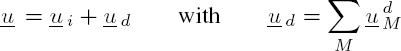
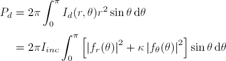
These regimes are characterized by a different dependence of the scattered power (as a function of frequency) and acoustic intensity (depending on the direction). These variations are expressed by two scattering cross-sections, which we define first in the case of a sphere. Using Iinc to denote the acoustic intensity (power per unit area) transported by the incident wave, the scattering cross-section σ is such that the product σIinc is equal to the total power Pd scattered throughout the space.
This one is obtained by integrating the scattered intensity Id(r, θ, ϕ) on a sphere, of very large radius r, surrounding the particle:

σ is homogeneous to a surface and independent of r, because, in the far field, the intensity of the scattered waves decreases as 1/r2. This quantity is usually normalized with respect to the dimensions of the scatterer. In the case of a rigid (in acoustics) or opaque (in optics) sphere, whose radius R is very large compared to the wavelength λ, and for a directional beam, it is natural to assume that, in the absence of absorption, the scattered power corresponds to the rays intercepted by the particle, that is, πR2Iinc. Indeed, since σ is calculated at infinity, any ray, even a very slightly deflected one, leaves the geometric shadow cast by the obstacle. This is the case of waves diffracted by the disk of radius R, whose power is also equal to πR2Iinc. Indeed, we will see that, when kR approaches infinity, the scattering theory leads to a cross-section twice that predicted by the purely geometrical approach.
When the radius R is of the order of the wavelength, resonances and/or interference between the incident wave and the forward scattered waves considerably increase the efficiency of the scattering. This regime, described by the Mie theory in optics, is called resonant. Let us note that in acoustics the phenomena are more complex, especially in the case of an elastic scatterer buried in a solid matrix.
In order to characterize the scattering anisotropy, it is necessary to introduce a differential scattering section σd(θ, ϕ), such that:

Given the relation [2.2] and the 1/r2 decay of the scattered intensity, σd only depends on the direction defined by the polar angles θ and ϕ.
In the case of a cylinder, infinite and homogeneous along the z axis, the scattered acoustic intensity Id(r, θ) decreases as 1/r in the far field. The previous relations are replaced by:
where:
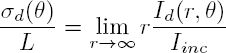
is the differential cross-section per unit length of the cylinder.
In the first section, entitled acoustic scattering, the scatterer is a cylinder immersed in a perfect fluid, therefore, the incident wave is longitudinal. Two cases are studied: a rigid cylinder and an elastic cylinder. In the second section, the elastic scattering by a cylinder embedded in an isotropic solid matrix is illustrated by a practical example for a longitudinal and a transverse incident wave. The scattering by a rigid or an elastic sphere buried in an isotropic solid matrix is treated in the third section. For both types of incident waves, the scattering cross-sections are calculated and their variations are illustrated in typical configurations. The phenomena of multiple scattering by a set of particles are discussed at the end of the chapter, using only a scalar approach.
2.1. Acoustic scattering by an immersed cylinder
In this section, we study the scattering of an acoustic wave by an infinitely long cylinder, of radius R, immersed in a fluid. The propagation is analyzed for time-harmonic waves of angular frequency ω and the time dependence in e−iωt is deliberately omitted. Let Rc be the cylindrical coordinate system (r, θ, z) of Appendix 1. The Cartesian coordinates are then defined in terms of cylindrical coordinates by relations [A1.1]. The field, contained in the xy plane, is independent of the z coordinate. The incident plane wave propagates in the x direction in a fluid of velocity Vf and mass density ρf. The velocity potential Φi associated with the incident wave, of amplitude af, is expanded on the cylindrical harmonics [A1.20]:
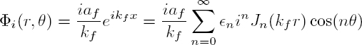
where Jn is the Bessel function of the first kind and where ϵn = 1 for n = 0 and ϵn = 2 for n > 0. The velocity potential of the wave scattered by the cylinder is also expanded on the cylindrical harmonics:

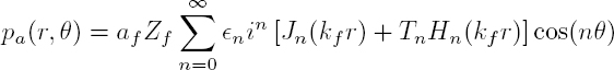
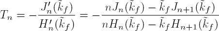
where ![]() is the Hankel function of the first kind, associated with a divergent wave. The amplitudes Tn of the cylindrical harmonics are to be determined from the boundary conditions. The total pressure and the radial velocity in the fluid are deduced from formulae [1.3] and [1.4]:
is the Hankel function of the first kind, associated with a divergent wave. The amplitudes Tn of the cylindrical harmonics are to be determined from the boundary conditions. The total pressure and the radial velocity in the fluid are deduced from formulae [1.3] and [1.4]:
and:

where the derivatives ![]() of the Bessel and Hankel functions are given by relations [A1.14].
of the Bessel and Hankel functions are given by relations [A1.14].
The separation of variables method thus leads to express the acoustic fields in the form of modal developments. These developments are convergent series. Apart from the monopolar mode (n = 0) and the dipolar mode (n = 1), the contribution of the nth order mode to this series is preponderant, as long as n is less than the reduced wave number kR. For numerical reasons, the series may therefore be truncated and the number of modes to consider for a satisfactory convergence depends on the frequency domain. At low frequencies, that is, when kR < 1, only the monopolar and dipolar modes have a significant influence. It is, therefore, usual to retain only these two modes, which leads to simpler analytical developments.
2.1.1. Scattering by a rigid cylinder
If the cylinder is immobile and rigid, the radial component of the particle velocity cancels on its surface: vr(r = R, θ) = 0. Taking into account the expression [2.9], this condition leads to the relation:
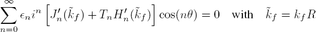
Given the orthogonality of the cos(nθ) functions, for each cylindrical harmonic we get:
Given the expression [A1.14] for the derivative of Bessel and Hankel functions, the scattering coefficients Tn can be written as:
In order to calculate the scattering cross-section, the solutions must be expressed in the far field. Since the Hankel function of the first kind and its derivative have the following asymptotic behavior:

the radial velocity and acoustic pressure associated with the scattered wave are given by the approximate expressions:

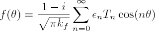
where the far-field scattering function f (θ) is equal to:
The scattered acoustic intensity is the time-average of the radial component of the Poynting vector:
In the far-field, Id is proportional to the intensity of the incident plane wave Iinc:

and where:
is the differential scattering cross-section, defined by equation [2.5]. The scattering cross-section corresponds to the average of σd(θ) on a cylindrical surface of very large radius r:
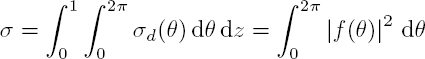
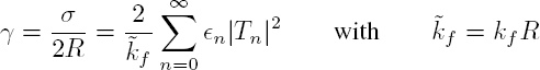
Since the cylinder is uniform and infinitely long, the integration along z is limited to the unit length. Upon normalizing with respect to the geometric cross-section 2R of the cylinder of unit length, the substitution of the expression [2.15] of the far-field scattering function f (θ) into relation [2.19] leads to:
In the long wavelength regime, that is for ![]() the summation appearing in the far-field scattering function f (θ) can be restricted to the first two modes. In this case, the scattering coefficients are given by the approximate expressions:
the summation appearing in the far-field scattering function f (θ) can be restricted to the first two modes. In this case, the scattering coefficients are given by the approximate expressions:
and the normalized differential cross-section σd/2R varies as (R/λ)3 in the Rayleigh scattering regime:
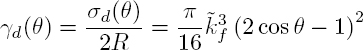
At high frequencies ![]() the normalized differential cross-section can be approximated by:
the normalized differential cross-section can be approximated by:
where the first term is a geometrical term representing the reflection by the cylinder, and the second one is a corrective term on the main lobe (Morse and Feshbach 1953).
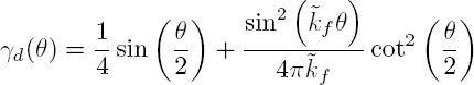
The differential cross-section is plotted in Figure 2.3 as a function of angle θ for different values of the product ![]() In each figure, the arrow indicates the propagation direction of the incident wave. At low frequencies, the differential scattering cross-section is small for θ = 0 and maximum for θ = π: the scattering takes place backward. Conversely, at high frequencies, the differential scattering cross-section is small for θ = π and maximum for θ = 0: the scattering takes place forward. This result, which can be surprising, a priori, is explained in the following paragraph.
In each figure, the arrow indicates the propagation direction of the incident wave. At low frequencies, the differential scattering cross-section is small for θ = 0 and maximum for θ = π: the scattering takes place backward. Conversely, at high frequencies, the differential scattering cross-section is small for θ = π and maximum for θ = 0: the scattering takes place forward. This result, which can be surprising, a priori, is explained in the following paragraph.
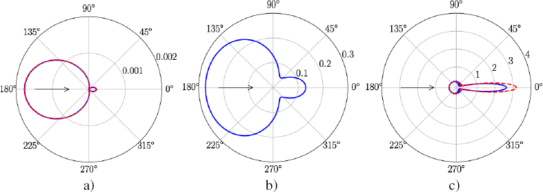
Figure 2.3. Normalized differential scattering cross-section for a rigid cylinder of radius R and unit length, immersed in a fluid. a)  f = 0.1, b) f = 1 and c) f = 10
Figure 2.4 depicts the interaction, at high frequency ![]() of a longitudinal plane wave with a rigid cylinder. The map of the scattered pressure field (Figure 2.4(a)) illustrates the magnitude of the forward emission lobe shown in Figure 2.3(c). On the map of the total pressure field (Figure 2.4(b)), there is clearly a shadow area behind the cylinder. It results from the destructive interference between the incident and scattered fields, which have almost the same amplitude, and are opposite in phase. The power scattered toward the front is, therefore, equal to 2RIinc. The second part of the scattered power comes from the reflection (clearly visible in Figure 2.4(a)), which corresponds to the geometric term in expression [2.23]. The integration over θ shows that it also contributes for 2R to the scattering cross-section of the cylinder, whose total value is twice its geometric cross-section. This contradiction between geometrical acoustics and scattering theory only exists at high frequency. When the dimensions of the scatterer are small, with respect to the wavelength, the scattered field is a small perturbation of the incident field. This “paradox”, explained by Brillouin (1949), arises from a contradiction between the intuitive association of the term “scattered” with “reflected”, and the mathematical definition of the scattered field, which includes both the reflected field as well as a term that interferes with the incident field to create the shadow behind the object. Difficulties arise when we try to interpret the results of the scattering theory through intuitive concepts.
of a longitudinal plane wave with a rigid cylinder. The map of the scattered pressure field (Figure 2.4(a)) illustrates the magnitude of the forward emission lobe shown in Figure 2.3(c). On the map of the total pressure field (Figure 2.4(b)), there is clearly a shadow area behind the cylinder. It results from the destructive interference between the incident and scattered fields, which have almost the same amplitude, and are opposite in phase. The power scattered toward the front is, therefore, equal to 2RIinc. The second part of the scattered power comes from the reflection (clearly visible in Figure 2.4(a)), which corresponds to the geometric term in expression [2.23]. The integration over θ shows that it also contributes for 2R to the scattering cross-section of the cylinder, whose total value is twice its geometric cross-section. This contradiction between geometrical acoustics and scattering theory only exists at high frequency. When the dimensions of the scatterer are small, with respect to the wavelength, the scattered field is a small perturbation of the incident field. This “paradox”, explained by Brillouin (1949), arises from a contradiction between the intuitive association of the term “scattered” with “reflected”, and the mathematical definition of the scattered field, which includes both the reflected field as well as a term that interferes with the incident field to create the shadow behind the object. Difficulties arise when we try to interpret the results of the scattering theory through intuitive concepts.
Figure 2.4. Interaction of a plane wave with a rigid cylinder immersed in water. a) Scattered field when f = 10. b) Superposition of the incident and scattered fields. For a color version of this figure, see www.iste.co.uk/royer/waves2.zip
2.1.2. Scattering by an elastic cylinder
The scattering by an isotropic elastic cylinder involves calculations similar to those developed for a rigid cylinder, but taking into account the longitudinal and transverse waves transmitted inside the cylinder. The cylinder material is characterized by its mass density ρ and its Lamé constants λ and μ, so that the longitudinal and transverse wave velocities are: ![]() The solution to the propagation equation is searched using the Helmholtz decomposition (equation [1.77] of Volume 1):
The solution to the propagation equation is searched using the Helmholtz decomposition (equation [1.77] of Volume 1):
where the scalar potentials ΦL and ΦT for longitudinal and transverse waves, polarized in the xy plane, are solutions to the Helmholtz equations (see section 1.2.6.1, Volume 1):
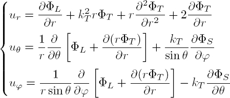
The displacement components are expressed in terms of ΦL and ΦT by the relations [1.126] in Volume 1:
Only stresses ![]() are involved in the boundary conditions. It is therefore necessary to express them, using formulae [A1.9] of Volume 1, as functions of the scalar potentials ΦL and ΦT :
are involved in the boundary conditions. It is therefore necessary to express them, using formulae [A1.9] of Volume 1, as functions of the scalar potentials ΦL and ΦT :
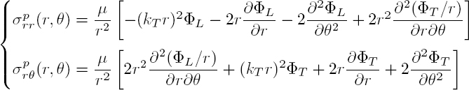
During the calculation, and in order to limit the order of the derivatives to one, the second derivatives of the potentials, with respect to r, have been eliminated using the Helmholtz equations.
In the fluid, the velocity potential Φi is defined by the development [2.6]. Since v = − grad Φi = − iωu, and in order to be equivalent, the displacement potentials in the solid must be divided by iω. Consequently, the scalar potentials ΦL and ΦT, associated with longitudinal and transverse waves, respectively, are given by Faran (1951):
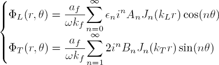
The potential of the transverse wave, transmitted in the cylinder, is expressed as a function of sin(nθ), while the potential of the longitudinal waves (incident, scattered, and transmitted) is expressed as a function of cos(nθ). This difference can be explained by the derivative operation according to θ and applied to the potential ΦT in relations [2.26] and [2.27] giving the displacement ![]() and the stress
and the stress ![]() From the expressions for the potentials, the normal displacement
From the expressions for the potentials, the normal displacement ![]() and the stresses
and the stresses ![]() and
and ![]() take the following forms at r = R:
take the following forms at r = R:
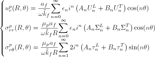
with:
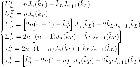
and where ![]()
The boundary conditions on the cylinder surface r = R are:

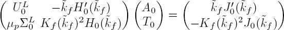
The substitution in the boundary conditions of the expressions of the pressure [2.8] and the radial velocity [2.9] in the fluid, as well as the displacements and stresses [2.29] in the solid, leads to a system of three equations with an infinite number of unknowns: the scattering coefficients An, Bn and Tn. Given the orthogonality of functions cos(nθ) and sin(nθ), for the harmonic n = 0 these equations are reduced to the following system:
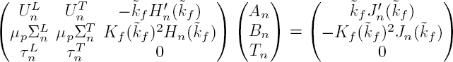
and for each harmonic of order n > 0:
The resolution of this system provides the scattering coefficient Tn for the waves in the fluid and, as in the previous section, the scattering cross-section. Its normalized value γ (formula [2.20]) is plotted in Figure 2.5 for three different cylinders: a rigid cylinder, a steel cylinder and a plexiglass cylinder. The scattering cross-section for the steel cylinder is relatively close to that of the rigid cylinder because its elastic moduli are very high. However, several peaks appear that correspond to resonances. There are many more resonances for the plexiglass (PMMA) cylinder, whose elastic parameters are relatively close to the bulk modulus of water ![]() GPa. Some resonances are related to the propagation of elastic waves on the surface of the scatterer.
GPa. Some resonances are related to the propagation of elastic waves on the surface of the scatterer.

Figure 2.5. Normalized scattering cross-section γ for a rigid cylinder, a steel cylinder and a plexiglas (PMMA) cylinder, immersed in water. For a color version of this figure, see www.iste.co.uk/royer/waves2.zip
2.1.3. Circumferential waves
In the harmonic case, these waves are the solutions, finite at the origin, to the Helmholtz equations [2.25], propagating on the surface of the cylinder. The potentials ΦL and ΦT are given by equation [A1.17], by replacing Rn with Bessel functions of the first kind Jn, that is, for the mode of order n:

These exponential solutions represent waves propagating anticlockwise at the phase velocity V = ωR/n. Assuming that the surface of the cylinder is traction free, the stresses σrr and σrθ must be canceled for r = R, that is, given expressions [2.29]:

By taking into account expressions [2.30] of coefficients ![]() the characteristic equation takes the form:
the characteristic equation takes the form:
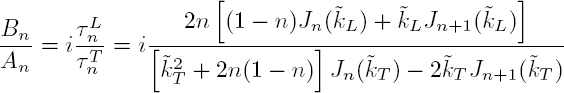
and the ratio of the amplitudes of the potentials, for n ≠ 0, is given by:
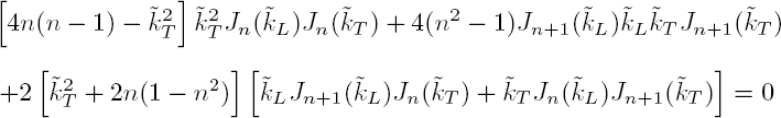
The characteristic equation [2.36] is solved by denoting:
For each value of n, there exists an infinite number of solutions xm, to which correspond the angular frequencies ωn,m = VT xm/R. For each mode, the components ur and uθ of the mechanical displacement are deduced from the relations [2.26]. When n = 0 and since ![]() equation [2.35] is written as
equation [2.35] is written as ![]() Equation
Equation ![]() is identical to the relation [4.194] in Volume 1 that gives the cut-off frequencies for the radial modes of a cylinder. Equation
is identical to the relation [4.194] in Volume 1 that gives the cut-off frequencies for the radial modes of a cylinder. Equation ![]() is identical to the dispersion equation [4.199] of Volume 1, for the torsional modes, polarized along eθ. The radial and tangential components of the mechanical displacement are decoupled.
is identical to the dispersion equation [4.199] of Volume 1, for the torsional modes, polarized along eθ. The radial and tangential components of the mechanical displacement are decoupled.
Figure 2.6(a) shows the variations in the normalized frequency ωR/VT versus the angular wave number kR for the steel cylinder. The integer values n of kR satisfy a phase matching condition at each revolution: Δϕ = 2πkR = 2nπ and thus correspond to a resonance. For n ≥ 1, the calculation of the components ur and uθ shows that the first root ωn,0 corresponds to a mechanical disturbance localized near the surface, which becomes a Rayleigh wave when n = kR → ∞, that is, for a cylinder whose radius is very large compared to the wavelength. The other solutions (m = 1, 2, etc.) correspond to the so-called “whispering gallery modes”, also discovered by Lord Rayleigh, and whose mechanical displacement is more concentrated inside the cylinder. When kR approaches unity, the frequency, and thus the phase velocity of the mode m = 0 cancel out (Figure 2.6(b)). The dispersion effect due to the curvature of the surface is quite large at low frequencies (kR < 10), that is, when the wavelength is larger than R/2. When kR tends to infinity, the phase velocity V = ω/k approaches the velocity VR of the Rayleigh wave on a plane surface. It must be noted that the non-integer values of kR are involved in the transient regime to describe the non-resonant propagation of a surface disturbance around the cylinder. The number of turns is then limited by the material attenuation, the diffraction and the dispersion, which cause the wave packet to spread out.

Figure 2.6. a) Dispersion curves of the Rayleigh mode (m = 0) and whispering gallery modes (m ≥ 1) on the free surface of a steel cylinder. The discrete values correspond to the resonance frequencies ωn,m. b) Phase velocity of the Rayleigh wave as a function of kR. For a color version of this figure, see www.iste.co.uk/royer/waves2.zip
The position of the first circumferential modes (n,m), indicated in Figure 2.5, is in good agreement with the resonances of the scattering cross-section in the steel cylinder. Given its very small acoustic impedance, the presence of water causes little disturbance in the propagation of waves on the surface of the steel cylinder. This is no longer true for the plexiglass cylinder, and the characteristic equation of the interface waves are thus obtained by canceling the determinant of the system [2.33].
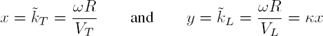
2.2. Scattering of elastic waves by a cylinder
In this section, the scatterer is an elastic cylinder embedded in an isotropic solid matrix. The displacements in the matrix and cylinder are calculated using the Helmholtz decomposition [2.24]. Let aI (I = L, T) be the amplitude of the displacement potential for the incident plane wave (longitudinal or transverse) propagating in the x direction. Since x = r cos θ, the Jacobi and Anger development [A1.18] leads to the expression:

The potential associated with a scattered wave takes the form:
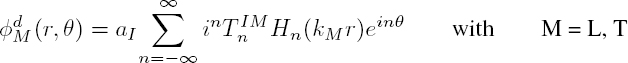
where the scattering coefficient ![]() represents the amplitude of the cylindrical harmonic n of the scattered mode M for an incident wave of type I. The calculation of the scattering coefficients involves the boundary conditions on the cylinder surface r = R. This requires the calculation of displacements and stresses, given by the expressions [2.26] and [2.27], respectively.
represents the amplitude of the cylindrical harmonic n of the scattered mode M for an incident wave of type I. The calculation of the scattering coefficients involves the boundary conditions on the cylinder surface r = R. This requires the calculation of displacements and stresses, given by the expressions [2.26] and [2.27], respectively.
For an incident wave of type I (L or T), the differential scattering cross-section is the sum of two terms: σd = σL + σT, with:
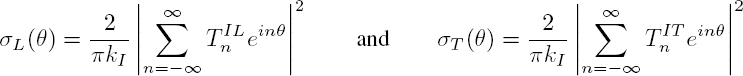
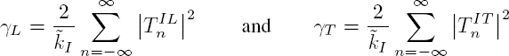
Given the orthogonality of the trigonometric functions, the scattering cross-sections normalized by the geometric cross-section of the scatterer can be written as:
Scattering by a glass cylinder buried in an epoxy matrix is illustrated in Figure 2.7. The differential scattering cross-sections into longitudinal and transverse waves are plotted in the case of a longitudinal incident wave and for two values of the dimensionless wave number ![]() The behavior of the scattered longitudinal wave is comparable with that of the acoustic wave scattered by an immersed cylinder. At low frequency
The behavior of the scattered longitudinal wave is comparable with that of the acoustic wave scattered by an immersed cylinder. At low frequency ![]() the scattering is weak and mainly takes place backward (decreasing x). At medium frequency
the scattering is weak and mainly takes place backward (decreasing x). At medium frequency ![]() backward and forward (increasing x) scattering are comparable. The converted transverse waves behave similarly, but their scattering is oriented at ±40◦ with respect to the propagation direction. Further, it is interesting to note that at low frequency, the differential scattering cross-section of the transverse wave is twice that of the longitudinal wave. More generally, the conversion of a longitudinal wave into a transverse wave is significant at low frequencies, as long as the cylinder is more rigid than the matrix.
backward and forward (increasing x) scattering are comparable. The converted transverse waves behave similarly, but their scattering is oriented at ±40◦ with respect to the propagation direction. Further, it is interesting to note that at low frequency, the differential scattering cross-section of the transverse wave is twice that of the longitudinal wave. More generally, the conversion of a longitudinal wave into a transverse wave is significant at low frequencies, as long as the cylinder is more rigid than the matrix.
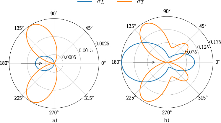
Figure 2.7. Longitudinal incident wave. Differential scattering cross-sections for a glass cylinder in an epoxy matrix at a frequency such that a) 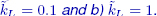 For a color version of this figure, see www.iste.co.uk/royer/waves2.zip
The differential scattering cross-sections into longitudinal and transverse waves are plotted in Figure 2.8 in the case of a transverse incident wave for two values of the dimensionless wave number ![]() The transverse wave is scattered along three main directions: backward and in two directions close to the y axis, perpendicular to the propagation direction. The converted longitudinal waves have the same behavior as the converted transverse waves presented in Figure 2.7, but with much smaller amplitudes (Liu et al. 2000). Wave conversion is thus smaller in the case of the transverse incident wave.
The transverse wave is scattered along three main directions: backward and in two directions close to the y axis, perpendicular to the propagation direction. The converted longitudinal waves have the same behavior as the converted transverse waves presented in Figure 2.7, but with much smaller amplitudes (Liu et al. 2000). Wave conversion is thus smaller in the case of the transverse incident wave.
The variation of the scattering cross-sections versus frequency is shown in Figure 2.9 for a longitudinal and a transverse incident wave. As previously indicated, the wave conversion in the case of the longitudinal wave is significant at low frequency, that is, for ![]() At higher frequencies, the scattering cross-section γT presents an oscillatory behavior whose period is
At higher frequencies, the scattering cross-section γT presents an oscillatory behavior whose period is ![]() (Figure 2.9(b)).
(Figure 2.9(b)).

Figure 2.8. Transverse incident wave. Differential scattering cross-section for a glass cylinder in an epoxy matrix at a frequency such that a)  T = 0.1 and b) T = 1. For a color version of this figure, see www.iste.co.uk/royer/waves2.zip
Figure 2.9. Scattering cross-sections for a glass cylinder in an epoxy matrix. a) Longitudinal and b) transverse incident wave. For a color version of this figure, see www.iste.co.uk/royer/waves2.zip
ORDER OF MAGNITUDE.– For a glass fiber of diameter 10 μm and a frequency f = 5 MHz, the reduced wave numbers are ![]() L = 0.13 and
L = 0.13 and ![]() T = 0.29. In the case of an epoxy resin matrix and a longitudinal incident wave, the normalized scattering cross-sections are small: γL = 0.004 and γT = 0.012; for a transverse incident wave, the corresponding values are γT = 0.05 and γL = 0.005.
T = 0.29. In the case of an epoxy resin matrix and a longitudinal incident wave, the normalized scattering cross-sections are small: γL = 0.004 and γT = 0.012; for a transverse incident wave, the corresponding values are γT = 0.05 and γL = 0.005.
2.3. Scattering of elastic waves by a spherical particle
In the first section, we give the general expressions of the displacement components and mechanical stresses in terms of the scalar potentials. In the second and third sections, we analyze successively the interaction of a longitudinal and a transverse elastic wave with a spherical particle embedded in an isotropic matrix. The scattering by a rigid particle is first investigated and then the scattering by a gaseous or a solid elastic inclusion.
2.3.1. General formulation of the problem
Let Rs be the spherical coordinate system (r, θ, ϕ) presented in Appendix 1. The Cartesian coordinates are then defined in terms of the spherical coordinates by relations [A1.21]. The displacement field u is searched using the Helmholtz decomposition [1.186], where ΦL, ΦT and ΦS are the scalar potentials, solutions to the Helmholtz equations [2.25].
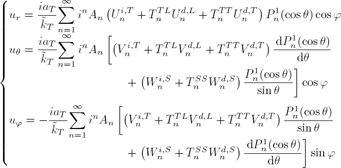
Considering expressions [A1.11] and [A1.15] in Volume 1 for the operators grad and rot in spherical coordinates, the components of the mechanical displacement are expressed as
Only the stresses σrr, σrθ and σrϕ are involved in the boundary conditions. It is therefore necessary to express these three components in terms of the scalar potentials ΦL, ΦT and ΦS using formulae [A1.17] of Volume 1:
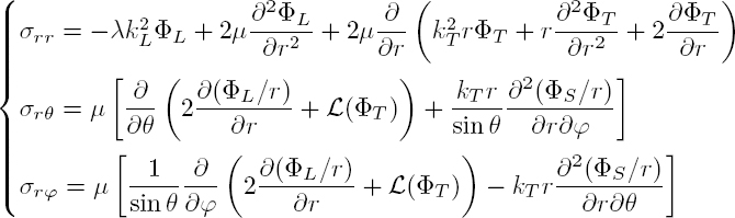
with:
In the following section, the potentials of the incident and scattered waves are developed over spherical harmonics. In Appendix 1, these harmonics are expressed using spherical Bessel functions and Legendre polynomials.
2.3.2. Scattering of a longitudinal plane wave
The case of a rigid sphere is treated first, in order to illustrate the decomposition of the incident and scattered fields on the spherical harmonics, as well as the use of orthogonality relations to calculate the scattering coefficients. The scattering by an elastic particle is then studied in the low-frequency domain, where monopolar and dipolar resonances appear. In the final section, the scattering cross-sections and the far-field scattering functions are calculated using approximations that are valid in the far field.
2.3.2.1. Scattering by a rigid particle
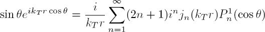
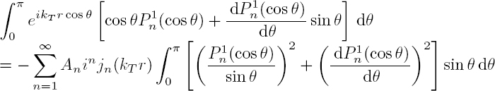
The incident wave is a longitudinal plane wave propagating in the z direction with the scalar potential ![]() and the displacement ui = aL exp(ikLz)ez. As z = r cos θ, the incident wave does not depend on angle ϕ. Its potential may be developed over spherical harmonics of order m = 0, according to the formula [A1.48]:
and the displacement ui = aL exp(ikLz)ez. As z = r cos θ, the incident wave does not depend on angle ϕ. Its potential may be developed over spherical harmonics of order m = 0, according to the formula [A1.48]:
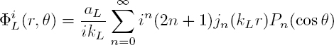
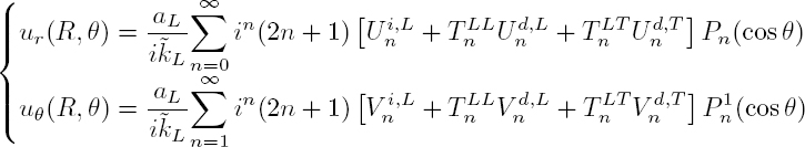
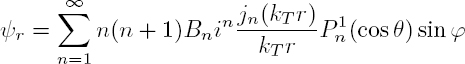
where jn and Pn are, respectively, the spherical Bessel functions of the first kind and the Legendre polynomials. Since the incident field is independent of angle ϕ, the scattered fields are also independent of ϕ. Moreover, the incident wave fronts, which are parallel to the xy plane (Figure 2.2(b)), impose that the displacement component uϕ is zero. Given the expressions [2.43], the potential ΦS is necessarily zero: there is no scattering into the transverse wave polarized in the xy plane. The potentials of the scattered longitudinal and transverse waves are also developed on the spherical harmonics:
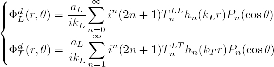
where ![]() are the scattering coefficients for longitudinal and transverse waves, respectively. Note that
are the scattering coefficients for longitudinal and transverse waves, respectively. Note that ![]() is the spherical Hankel function of the first kind and order n corresponding to a divergent wave. For the transverse wave, the sum must necessarily start from the term n = 1 because there is no monopolar transverse wave (Volume 1, section 1.2.6.2). By writing
is the spherical Hankel function of the first kind and order n corresponding to a divergent wave. For the transverse wave, the sum must necessarily start from the term n = 1 because there is no monopolar transverse wave (Volume 1, section 1.2.6.2). By writing ![]() L = kLR and
L = kLR and ![]() T = kT R, the expressions for the non-zero components of the displacement at r = R are:
T = kT R, the expressions for the non-zero components of the displacement at r = R are:
with ![]() and:
and:

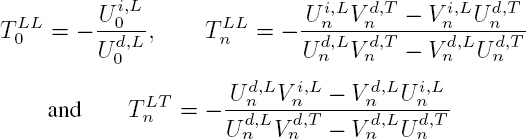
For the incident wave (p = i), the function fn is the spherical Bessel function of the first kind jn, while for the scattered waves (p = d), fn is the spherical Hankel function of the first kind hn. Since the particle is rigid, the displacements are zero on the surface r = R, leading to the system:

The orthogonality relation [A1.41] for the Legendre functions allows us to decouple this system into one system for each spherical harmonic:

The scattering coefficients are then given by the relations (Gaunaurd and Überall 1976):
At low frequencies, the scattering coefficients of the monopolar (n = 0) and dipolar (n = 1) modes are dominant in the modal series. By performing a limited development of spherical Bessel and Hankel functions for ![]() L << 1, the scattering coefficients of these modes are approximately written as (Valier-Brasier et al. 2015):
L << 1, the scattering coefficients of these modes are approximately written as (Valier-Brasier et al. 2015):

2.3.2.2. Scattering by an elastic particle
In the case of a particle with mass density ρp and Lamé constants λp and μp, the transmission of the longitudinal and transverse waves inside the particle must necessarily be taken into account in the modeling. To do this and using the Helmholtz decomposition [1.186] with ΦS = 0, the potentials of waves transmitted in the particle are searched in the form of expansions on spherical harmonics:
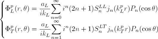
The transmission coefficients of the waves in the particle ![]() and the scattering coefficients in the matrix,
and the scattering coefficients in the matrix, ![]() (see equation [2.47]), are determined by the boundary conditions.
(see equation [2.47]), are determined by the boundary conditions.
At low frequency, that is, for ![]() L << 1, the scattering coefficients for the first two modes are given by Valier-Brasier et al. (2015):
L << 1, the scattering coefficients for the first two modes are given by Valier-Brasier et al. (2015):
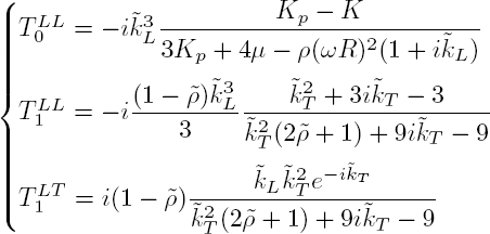
The monopolar mode (n = 0) depends directly on the difference between the bulk moduli of the two media ![]() while the dipolar (n = 1) mode depends on the density ratio
while the dipolar (n = 1) mode depends on the density ratio ![]() = ρp/ρ. These scattering coefficients exhibit very strong resonances at low frequency, whose frequencies correspond to the cancellation of the denominators of the scattering coefficients. Moreover, it is easy to verify that the scattering coefficients [2.53] of the rigid sphere are deduced from formulae [2.55], when the parameters of the scatterer (Kp and ρp) are very large compared to those of the matrix (K and ρ).
= ρp/ρ. These scattering coefficients exhibit very strong resonances at low frequency, whose frequencies correspond to the cancellation of the denominators of the scattering coefficients. Moreover, it is easy to verify that the scattering coefficients [2.53] of the rigid sphere are deduced from formulae [2.55], when the parameters of the scatterer (Kp and ρp) are very large compared to those of the matrix (K and ρ).
2.3.2.2.1. Monopolar resonance
This resonance occurs when the angular frequency ω cancels the denominator of the scattering coefficient ![]()
Assuming a rheology of Kelvin–Voigt type (equation [1.299] of Volume 1) for the shear modulus: μ = μ0 − iωη and by writing ![]() we get:
we get:
where:
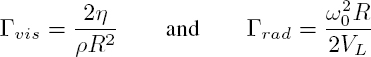
with:

The terms Γvis and Γrad express the viscosity and radiation losses, respectively. The resonance frequency f0 = ω0/2π, therefore, depends on the competition between the bulk modulus of the particle and the shear modulus of the host medium.
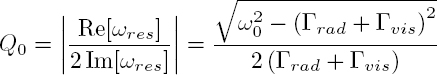
The complex resonance frequency, that is, the solution to equation [2.57], is given by:
and the quality factor can be written as:
If the particle is gaseous, its bulk modulus ![]() is small. For the air, Kp ≈ 140 kPa and the resonance is driven by the shear modulus of the solid. If the latter is too rigid, the resonance angular frequency ωres is high, as well as the term Γrad. The quality factor is then small: the resonance is not efficient. Conversely, for a soft solid, that is, with a shear modulus μ0 smaller than 100 MPa, the resonance occurs at a low frequency and the quality factor is high. However, for small bubbles (a few hundred μm), the resonance is located in the ultrasonic domain, that is, in the MHz range, where the effects of viscoelastic dissipation are significant and can no longer be represented by a Kelvin–Voigt model.
is small. For the air, Kp ≈ 140 kPa and the resonance is driven by the shear modulus of the solid. If the latter is too rigid, the resonance angular frequency ωres is high, as well as the term Γrad. The quality factor is then small: the resonance is not efficient. Conversely, for a soft solid, that is, with a shear modulus μ0 smaller than 100 MPa, the resonance occurs at a low frequency and the quality factor is high. However, for small bubbles (a few hundred μm), the resonance is located in the ultrasonic domain, that is, in the MHz range, where the effects of viscoelastic dissipation are significant and can no longer be represented by a Kelvin–Voigt model.
When the host medium is a viscous liquid, the static shear modulus μ0 is zero and the modulus η corresponds to the shear viscosity (section 1.5.5, Volume 1). The resonance frequency then takes the form:
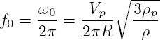
The resonance of a gas bubble in water, discovered by Minnaert, is very intense since its quality factor is very high:
ORDER OF MAGNITUDE.– For a gas bubble in water, the typical value of the product f0R is 3.26 m/s. The product ![]() L = 2πf0R/Vf ≈ 0.014 is very small in front of unity: the Minnaert resonance occurs at a very low frequency.
L = 2πf0R/Vf ≈ 0.014 is very small in front of unity: the Minnaert resonance occurs at a very low frequency.
2.3.2.2.2. Dipolar resonance
The dipolar resonance of an elastic particle occurs when the denominator of the corresponding scattering coefficients ![]() cancels out:
cancels out:
Assuming that ![]() the complex root of this equation is expressed by:
the complex root of this equation is expressed by:
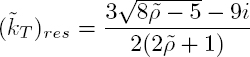
The resonance frequency and the quality factor [2.61] are thus given by Duranteau et al. (2016):

2.3.2.3. Scattering cross-section
For large arguments, the approximate expression for the spherical Hankel function of the first kind is given by [A1.40]. The substitution of the potentials [2.47] in equations [2.43] and [2.44] allows us to express the displacements ![]() and the stresses
and the stresses ![]() of the scattered wave in the far field:
of the scattered wave in the far field:
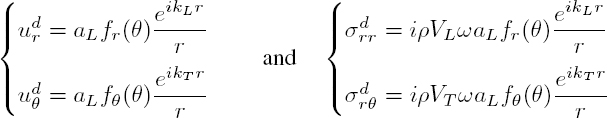
with:

The scattered acoustic intensity, defined by:

is written as follows in the far field, with ![]()
According to equation [2.2], the scattered power is the average intensity over a sphere of arbitrary large radius r:
The scattering cross-section σ = Pd/Iinc is the sum of two terms: σ = σL + σT. Using the orthogonality relation [A1.41], we get:
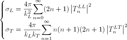
or again, by normalizing by the geometric cross-section of the scatterer S = πR2:
The scattering of a longitudinal plane wave by an elastic sphere buried in an epoxy resin is shown in Figure 2.10. The normalized cross-sections γL and γT have similar values in the case of the glass sphere and exhibit a maxima at slightly different frequencies. The scattering cross-section of a transverse wave for a lead sphere reaches a maximum value for the dimensionless wave number ![]() L ≈ 0.3, which corresponds to the dipolar resonance frequency f1 of the translational motion of the sphere in epoxy (Figure 2.10(b)). The scattering cross-section of the longitudinal wave is much smaller than that of the transverse wave, signifying that the energy carried by the incident wave is preferentially scattered into the transverse wave rather than into the longitudinal wave. It should be noted that each of these coefficients approaches unity at high frequency and, therefore, the total cross-section has a limit equal to 2πR2, as predicted.
L ≈ 0.3, which corresponds to the dipolar resonance frequency f1 of the translational motion of the sphere in epoxy (Figure 2.10(b)). The scattering cross-section of the longitudinal wave is much smaller than that of the transverse wave, signifying that the energy carried by the incident wave is preferentially scattered into the transverse wave rather than into the longitudinal wave. It should be noted that each of these coefficients approaches unity at high frequency and, therefore, the total cross-section has a limit equal to 2πR2, as predicted.

Figure 2.10. Longitudinal incident wave. Normalized scattering cross-section for a) a glass bead and b) a lead bead, buried in an epoxy resin
The moduli of the far-field scattering functions, fr and fθ, are plotted in the case of a glass bead for ![]() L = 4.3 (Figure 2.11(a)) and a lead bead for
L = 4.3 (Figure 2.11(a)) and a lead bead for ![]() L = 0.3 (Figure 2.11(b)). For the glass bead, the far-field scattering function fr, which depends only on the scattering coefficients
L = 0.3 (Figure 2.11(b)). For the glass bead, the far-field scattering function fr, which depends only on the scattering coefficients ![]() is highly directional: the longitudinal scattering takes place in the forward direction. In contrast, the scattering of the transverse wave, represented by the function fθ, is less directional and much smaller. For the lead bead, the two far-field scattering functions present dipolar behavior (Figure 2.11(b)). This result is quite logical, given that these functions are calculated at the translational resonance frequency f1 of the particle. On the other hand, the waves are scattered in different directions: scattering takes place preferentially in the propagation direction for the longitudinal wave, while it occurs perpendicularly for the transverse wave. This behavior results from the translational motion of the solid bead, which follows the polarization of the incident wave.
is highly directional: the longitudinal scattering takes place in the forward direction. In contrast, the scattering of the transverse wave, represented by the function fθ, is less directional and much smaller. For the lead bead, the two far-field scattering functions present dipolar behavior (Figure 2.11(b)). This result is quite logical, given that these functions are calculated at the translational resonance frequency f1 of the particle. On the other hand, the waves are scattered in different directions: scattering takes place preferentially in the propagation direction for the longitudinal wave, while it occurs perpendicularly for the transverse wave. This behavior results from the translational motion of the solid bead, which follows the polarization of the incident wave.
2.3.3. Scattering of a transverse plane wave
The analysis of the scattering of a transverse wave by a spherical particle is more complicated than the scattering of an incident longitudinal wave, because of the polarization perpendicular to the propagation direction. The calculation of a transverse plane wave in the spherical coordinate basis is first carried out using Helmholtz decomposition, which requires two scalar potentials. The scattering by a rigid sphere is then examined; the decomposition of the incident and scattered fields on the spherical harmonics shows that one of the transverse waves is coupled with the converted longitudinal wave, while the other is decoupled. In the last section, the scattering cross-sections and far-field scattering functions are calculated and the resonances arising from the propagation of the Stoneley wave on the surface of a lead sphere are highlighted.
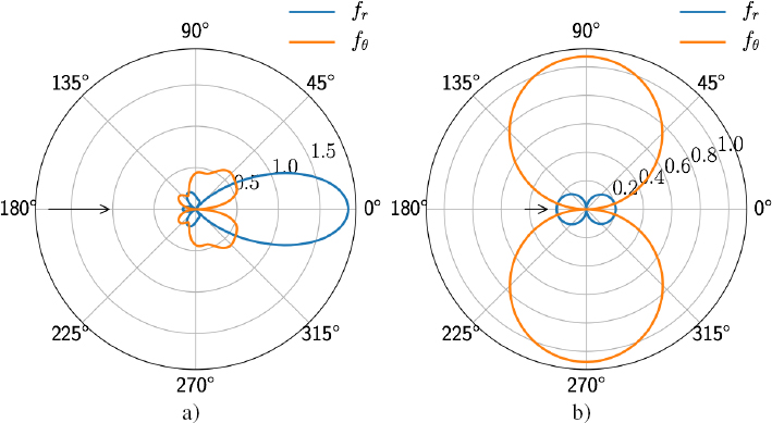
Figure 2.11. Far field scattering functions for a bead made of a) glass ( L = 4.3) and b) lead (L = 0.3) buried in an epoxy resin. The circles of equal amplitude are graduated in mm. For a color version of this figure, see www.iste.co.uk/royer/waves2.zip
2.3.3.1. Transverse incident plane wave
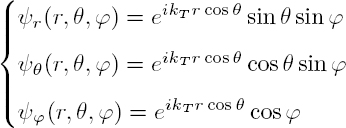
We are interested in the scattering by a sphere of a plane transverse wave propagating in the z direction and polarized along x. A vector potential parallel to y:
imposes a particle displacement u oriented in the x direction:
Given the expression for the vector ey:
the components of the vector ψ are defined in the spherical coordinate system through the relations:
The vector potential ψ is expressed in terms of two scalar potentials φT and φS by the relation [1.186]:
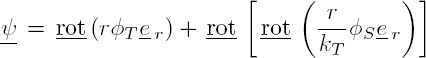
that is:

By analogy with the development [A1.48] of a plane wave, the scalar potentials φT and φS are expanded on the spherical harmonics ![]() or
or ![]() whose dependence on ϕ is similar to the dependence of ψθ and ψϕ, given the derivatives:
whose dependence on ϕ is similar to the dependence of ψθ and ψϕ, given the derivatives:
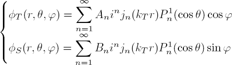
where the amplitudes An and Bn are to be identified. The spherical Bessel functions of the second kind are not taken into account in these two developments because they are not defined at r = 0. Knowing that the function ![]() is a solution to the associated Legendre equation [A1.29]:
is a solution to the associated Legendre equation [A1.29]:

the radial component of the potential ψ takes the form:
Given the spherical harmonic expansion [A1.48] of the plane wave and since P0(cos θ) = 1 and ![]() we get, after derivation with respect to θ:
we get, after derivation with respect to θ:
Comparing expressions [2.77] and [2.82] for the component ψr leads to:
Given the relation [2.77] and substituting the potentials [2.80] into the expressions [2.79] of ψθ and ψϕ leads to:

and:

The first term on the right-hand side of these two equations is eliminated by multiplying the first equation by ![]() and the second one by
and the second one by ![]() and then by integrating over θ, from 0 to π. Indeed, it appears the integral:
and then by integrating over θ, from 0 to π. Indeed, it appears the integral:
which is zero, since the Legendre functions are either even or odd. Adding each side of the transformed equations [2.85] and [2.86] leads to:
Using the spherical harmonic expansion [A1.48] of the plane wave and noting that the term between square brackets is equal to ![]() the integral of the left-hand side is calculated by parts:
the integral of the left-hand side is calculated by parts:
considering the normalization [A1.41] of the Legendre functions ![]() Given relation [A1.43], the equality of each term of the sum in equation [2.88] leads to:
Given relation [A1.43], the equality of each term of the sum in equation [2.88] leads to:
2.3.3.2. Scattering coefficients for a rigid sphere
The incident wave is a transverse plane wave propagating in the z direction with the vector potential Ψ i = (iaT /kT ) exp(ikT z)ey and mechanical displacement ui = aT exp(ikT z)ex. Three scattered waves are considered in the host medium; they are represented by the scalar potentials:
where the scattering coefficients ![]() are to be determined. The components of the mechanical displacement on the sphere surface are expressed by:
are to be determined. The components of the mechanical displacement on the sphere surface are expressed by:
where the coefficients ![]() with p = i, d and M = L, T, are given by expressions [2.49] and the coefficients
with p = i, d and M = L, T, are given by expressions [2.49] and the coefficients ![]() by:
by:
The use of the orthogonality relations [A1.41], [A1.43] and [A1.44] allows us to decouple the system resulting from the cancellation of the three displacement components, given by relations [2.92], into one system for each harmonic n:
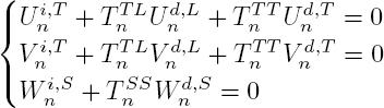
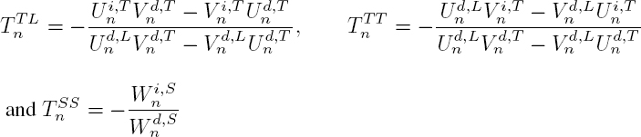
Since the third equation is independent of the first two, the transverse wave S is decoupled from the L and T waves. The scattering coefficients ![]() are expressed by:
are expressed by:
2.3.3.3. Scattering cross-section
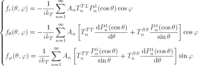
In the far field, considering expressions [2.43] and [2.44], the components of the displacement and stresses for the scattered field are expressed as:

with
Expression [2.69] for the scattered intensity takes the form:
with:
The scattered power is the average of Id(r, θ, ϕ) over a sphere of arbitrary large radius r. Integrating over angle ϕ from 0 to 2π amounts to multiplying each of the three terms by π:
with:

Given the orthogonality relations of the Legendre functions [A1.41] to [A1.44] and the normalization by πR2 and by the intensity Iinc of the incident plane wave, the scattering cross-sections ![]() are expressed by Einspruch et al. (1960):
are expressed by Einspruch et al. (1960):
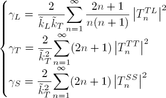
Figure 2.12 illustrates the scattering of a transverse plane wave by an elastic sphere buried in an epoxy resin. For the steel sphere (Figure 2.12(a)), the scattering cross-sections for the longitudinal and transverse T waves exhibit a maximum for the dimensionless wave number ![]() T ≈ 0.83, corresponding to the dipolar resonance frequency f1 of the translational motion of the sphere in epoxy. The scattering cross-section of the transverse S wave has a maximum for the dimensionless wave number
T ≈ 0.83, corresponding to the dipolar resonance frequency f1 of the translational motion of the sphere in epoxy. The scattering cross-section of the transverse S wave has a maximum for the dimensionless wave number ![]() T ≈ 1.32. This peak is associated with the rotational dipolar resonance of the particle. The same resonances are visible for the lead sphere (Figure 2.12(b)), but with larger amplitudes, since lead is denser than steel and therefore the quality factor [2.66] associated with its resonance is larger. In addition, it appears as a series of peaks, almost regularly spaced apart by a value Δ
T ≈ 1.32. This peak is associated with the rotational dipolar resonance of the particle. The same resonances are visible for the lead sphere (Figure 2.12(b)), but with larger amplitudes, since lead is denser than steel and therefore the quality factor [2.66] associated with its resonance is larger. In addition, it appears as a series of peaks, almost regularly spaced apart by a value Δ![]() T = 0.71 for higher orders. These resonances are due to the existence of a Stoneley wave propagating at the interface between the lead and the epoxy with the velocity VSto = 651 m/s when this interface is plane. This value, that is, the solution to the characteristic equation dSto = 0 ([3.128], Volume 1), is the limit of the velocity of the circumferential Stoneley wave, when kTR >> 1.
T = 0.71 for higher orders. These resonances are due to the existence of a Stoneley wave propagating at the interface between the lead and the epoxy with the velocity VSto = 651 m/s when this interface is plane. This value, that is, the solution to the characteristic equation dSto = 0 ([3.128], Volume 1), is the limit of the velocity of the circumferential Stoneley wave, when kTR >> 1.
Given the transverse velocity in epoxy VT = 953 m/s, the gap between two peaks, corresponding to Δ(kStoR) = 1 with kSto = ω/VSto, related to a complete turn around the sphere, tends to:

The characteristic equation dSto = 0 has no solution for the steel-epoxy couple. There is no Stoneley wave in this case, which explains the absence of resonances due to circumferential waves in Figure 2.12(a).
2.4. Scattering by a set of particles
A wave propagating in a heterogeneous medium is scattered by all obstacles it encounters. If the number of scatterers present on its path is small, the interactions between the fields scattered by each obstacle may not be taken into account. This simple scattering regime is used in certain imaging techniques based on the measurement of the paths of direct waves. If the wave encounters several obstacles, the multiple interactions between all the scattered fields lead to the multiple scattering regime. In a dilute medium, that is, with a low concentration of heterogeneities, coherent waves can be observed. These waves, which are the part of the field that is resistant to averaging over the disorder, are attenuated and their velocity is close to that of the host medium; they propagate as in a homogeneous medium, both dissipative and dispersive, called an effective medium.
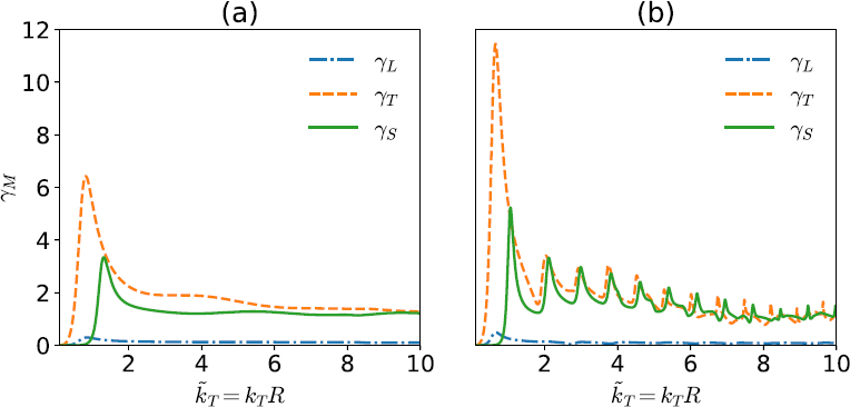
Figure 2.12. Transverse incident wave. Scattering cross-section for a) a steel bead and b) a lead bead, embedded in an epoxy resin. For a color version of this figure, see www.iste.co.uk/royer/waves2.zip
2.4.1. Scalar theory of multiple scattering
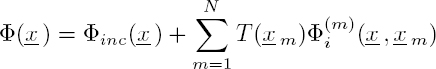
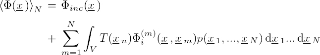
Let us study the propagation, in a heterogeneous medium, of a wave represented by the scalar potential Φinc, for example, a longitudinal wave in a perfect fluid. By hypothesis, the distribution is monodisperse in size and shape: the obstacles are all identical and randomly distributed in the volume V. The interaction of the incident wave with the N obstacles positioned at xm (with m = 1, .., N ) leads to the generation of N scattered waves of potentials ![]() . At point x, the potential representing the total field resulting from the propagation of all the waves may thus be written in the form:
. At point x, the potential representing the total field resulting from the propagation of all the waves may thus be written in the form:
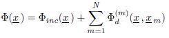
This potential takes into account the primary interactions between the incident wave and the obstacles but also all the secondary interactions between the fields scattered by each obstacle (Figure 2.13).
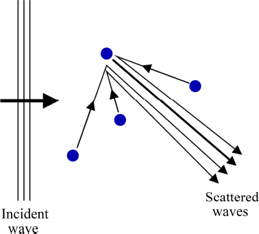
Figure 2.13. The field scattered by an obstacle at a point in space is the sum of the simple scattering (thick lines) and the waves that have undergone multiple scattering
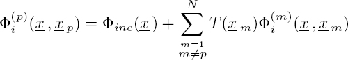
The incident field on the pth scatterer can be written as the sum of the incident field Φinc and the fields scattered by all the other obstacles:

The key for solving this problem is to determine the transition operator T (xp) that connects the incident field arriving at the pth scatterer to the field scattered by this obstacle:
Using this relation, without knowing, at this stage, the expression for T (xp), equations [2.104] and [2.105] are written in the form:
and:
Several strategies can be considered for solving the system of equations [2.107] and [2.108]. A first method consists of solving the problem by using the addition theorem to write the incident fields on each scatterer in its own reference frame (Rohfritsch et al. 2019). This procedure requires the inversion of large linear systems, which can generally only be done numerically. An example of the result is shown in Figure 2.14(a), which illustrates the field scattered by a plane wave propagating in the direction of increasing x and interacting with a random distribution of 400 steel cylinders immersed in water, between the two planes represented by the dashed vertical lines.
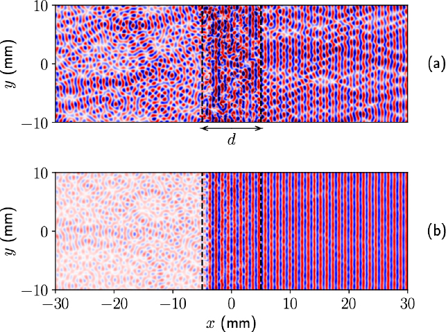
Figure 2.14. Field scattered by a set of steel cylinders immersed in water. a) Field for a random draw and b) field averaged over 20 draws. The cylinders are arranged between the two vertical planes depicted by the dashed lines. For a color version of this figure, see www.iste.co.uk/royer/waves2.zip
The field averaged over 20 different distributions of the positions of the cylinders is presented in Figure 2.14(b). This shows the creation of a coherent wave front, inside the layer, propagating in the direction of increasing x. This result illustrates another way to approach this problem, which consists of searching for the effective properties of coherent waves. For this purpose, the fields are averaged over all possible positions of the scatterers. In this perspective, let us consider a random distribution of N scatterers, characterized by a probability density function p(x1, x2,...,xN). The configurational average is defined by the relation:

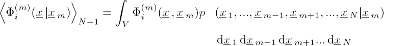
Physically, the average field ![]() is the statistical mean of the field f (x) over all possible positions of the scatterers in the volume V. The probability density function p(x1, ..., x N ) is put in the form:
is the statistical mean of the field f (x) over all possible positions of the scatterers in the volume V. The probability density function p(x1, ..., x N ) is put in the form:
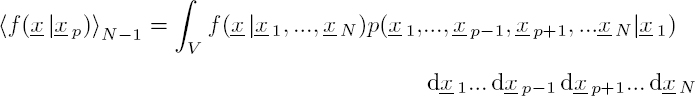
where p(x1, ..., x p−1, xp+1, ..., x N|xp) is the conditional probability density. This function represents the probability density for the presence of all scatterers, except the pth scatterer, which is fixed at xp. The configurational average with a fixed scatterer is defined by the relation:
Applying the configurational average [2.109] to relation [2.107] over all possible positions of the scatterers leads to the equation:
Using expressions [2.110] and [2.111], we get:

with:
The distribution being monodisperse, the probability density p(xm) is related to the number of scatterers per unit volume n(xm) through: n(xm) = Np(xm). Assuming a large number of scatterers, the Foldy–Lax approximation (Foldy 1945):
translates that the incident field on the fixed scatterer m, averaged over all possible positions of the other scatterers, is approximately equal to the averaged field. According to Twersky, this approximation leads us to neglect all the scattering loops between each pair of scatterers (Ishimaru 1978). Considering the Foldy–Lax approximation [2.115], relation [2.113] takes the form of the Foldy–Twersky equation (Foldy 1945):

Assuming a low concentration of localized scatterers, uniformly distributed, the number of scatterers per unit volume corresponds approximately to the average number of scatterers per unit volume n0 : n(xm) ≈ n0 and the transition operator can be expressed as:
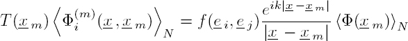
where f (ei, ej) is the far-field scattering function, calculated for a single scatterer. The vector ei is the unit vector in the propagation direction of ⟨Φ(xm)⟩N, while vector ej is the unit vector in the direction x− xm.
In the following, the Foldy–Twersky equation is solved in the case of perfectly spherical scatterers of radius R, contained within two parallel planes located at z = 0 and z = d (Figure 2.15). The distribution is random and uniform, and the particles do not interpenetrate each other.
The incident wave is a plane wave of unit amplitude, propagating in the z direction:
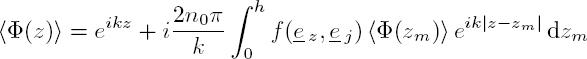
Considering that the coherent wave also propagates in the z direction, the substitution of expression [2.117] for the transition operator into the Foldy–Twersky equation [2.116] leads to the relation:

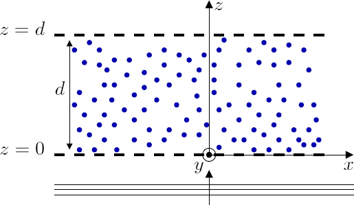
Figure 2.15. Layer of thickness d containing a random distribution of spherical scatterers
The double integral between square brackets is calculated by applying the stationary phase method, discussed in section 1.2.2.1, first to the variable xm and then to the variable ym :
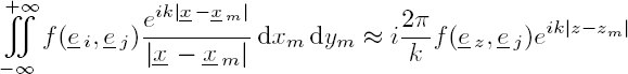
hence:
The vector ej is collinear to ez and its sign depends on the sign of z – zm. The integral is split into two parts:
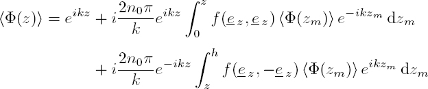
The first two terms of the right-hand side represent the propagation of progressive waves, while the third term represents the propagation of regressive waves. It then follows that the functions f (ez, ez) and f (ez, e z) correspond to the far-field scattering functions fr(0) and fr(π), representing, respectively, forward and backward scattering of a longitudinal wave. If the backward scattering is negligible compared to the forward scattering1, we get:
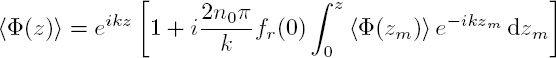
Upon multiplying this equation by e−ikz and by taking the derivative of the result with respect to z, the integral equation is reduced to a first-order differential equation:

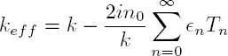
whose solution is a simple plane wave 〈Φ(z)〉 = eikeff z, with an effective wave number equal to:
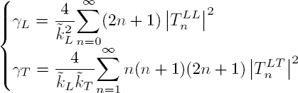
In the case of spherical scatterers, and given formula [2.68] with Pn(1) = 1 and kL = k, the expression for the effective wave number is:

where Tn is the scattering coefficient of order n for the longitudinal wave, that is, ![]()
In the case of cylindrical scatterers, the same reasoning leads to the relation:
The two previous expressions are approximations of the formulae:
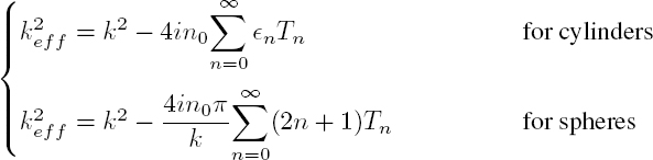
which are often attributed to Foldy, although this author considered point-like scatterers with isotropic radiation. They remain the simplest formulae giving the effective wave number. If backward scattering is not negligible, a reasoning similar to that just described leads to the effective wave number of Waterman and Truell (Waterman and Truell 1961). Moreover, formula [2.128] are still valid for longitudinal waves propagating in solids using the scattering coefficients ![]() instead of Tn. For shear coherent waves, the formula for cylinders remains valid by using the scattering coefficients
instead of Tn. For shear coherent waves, the formula for cylinders remains valid by using the scattering coefficients ![]() instead of Tn. However, in the three-dimensional case, due to the T and S polarizations, the effective wave number of coherent shear waves propagating in a dispersion of spherical particles embedded in a solid matrix is given by Tsang and Kong (1982):
instead of Tn. However, in the three-dimensional case, due to the T and S polarizations, the effective wave number of coherent shear waves propagating in a dispersion of spherical particles embedded in a solid matrix is given by Tsang and Kong (1982):
equation [2.113] was obtained by fixing a particle and by averaging over all possible positions of the other particles. This mathematical operation can be repeated for several particles, leading to a hierarchy of equations. However, if the number of particles N is large, it is preferable to break up this hierarchy by introducing an approximation. Previously, this hierarchy has been restricted to the first-order by using the independent scattering approximation (ISA). Lax (1952) introduced a second-order approximation, by performing the calculation for two fixed particles. This quasi-crystalline approximation (QCA) gives rise to several different expressions for the effective wave numbers. In particular, Fikioris and Waterman (1964) take into account the fact that two scatterers cannot interpenetrate by introducing the hole correction, which imposes an exclusion distance in the conditional probability density.
Following these works, many formulae, more or less complex, have been proposed to describe the propagation in a medium containing scatterers (Linton and Martin 2005; Conoir and Norris 2010). The advantage of approaches based on the multiple scattering theory lies in the simplicity of the expressions for the effective wave numbers because these only require the determination of scattering coefficients inherent to the problem being studied. However, these formulae are valid as long as the concentration of scatterers and the scattering cross-section remain small.
2.4.2. Velocity and attenuation of coherent waves
The properties of the coherent wave that can be measured are its phase velocity and its attenuation, defined by:
We will study these properties in two cases: a forest of immersed cylindrical rods and an elastic material containing a distribution of resonant spherical particles.
2.4.2.1. Propagation of coherent acoustic waves in a forest of cylindrical rods
Coherent waves propagating in a forest of cylindrical steel rods immersed in water were measured using the phase difference method introduced in section 2.4.2.4.2 of Volume 1. The rods, of diameter 1.5 mm, are distributed in a layer of thickness d = 15 mm and 20 cm wide. The sample is laterally displaced over thirty positions and transmission measurements are carried out for each position using circular piezoelectric transducers of diameter 13 mm and center frequency 2.25 MHz. The acquired signals are averaged in order to reduce the incoherent field. A reference signal sref (t), corresponding to the propagation from the emitter to the receiver, without the sample, is also acquired.
In order to observe the influence of averaging on the signal, the average signals savg and the first recorded signal s1(t) are shown in Figure 2.16(a). The moduli of the Fourier transforms of the average and reference signals, normalized by the maximum of the modulus of the reference signal spectrum, are shown in Figure 2.16(b). The vertical dashed lines delimit the frequency domain of the study. These limits are imposed to ensure the assumption of plane waves, which are necessary in the phase difference method. The minimum frequency is chosen in order to avoid diffraction by the edges of the sample due to the beam divergence (see section 1.1.4.3), and the maximum frequency is imposed so that the sample is located in the far field.
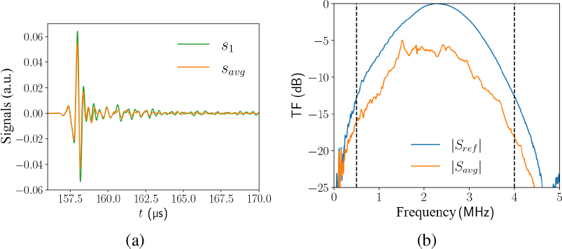
Figure 2.16. a) Raw signal s1(t) and averaged signal savg(t). b) Moduli of the Fourier transforms of the averaged signal (|Savg|) and reference signal (|Sref|), normalized by the maximum of the modulus of the Fourier transform of the reference signal. For a color version of this figure, see www.iste.co.uk/royer/waves2.zip
Since there is no physical interface, the phase velocity and attenuation of the coherent wave are given by relations [2.120] in Volume 1, with h = d, ρ = ρf, and ZL = Zf :

These quantities are plotted in Figure 2.17 as a function of the frequency for a plate containing a random distribution of steel cylinders, of concentration φ = 15%. The experimental results are compared to expression [2.128], as well as to the Fikioris and Waterman model (1964), which is a second-order approximation with respect to the concentration. Its first-order term is the same as that in relation [2.128]. This comparison shows, for the velocity and attenuation, that the second-order term in concentration must be taken into account in the modeling (Derode et al. 2006). These results must be compared with the scattering cross-section of a single steel cylinder immersed in water, as depicted in Figure 2.5. The attenuation and phase velocity are strongly impacted by the propagation of circumferential waves (see section 2.1.3).
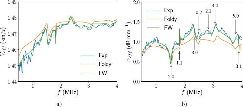
Figure 2.17. a) Phase velocity and b) attenuation of the coherent wave versus frequency, in a distribution of steel cylinders immersed in water. The arrows indicate the position of the circumferential waves. For a color version of this figure, see www.iste.co.uk/royer/waves2.zip
2.4.2.2. Propagation of coherent longitudinal waves in a dispersion of beads
The velocity and attenuation of the coherent longitudinal wave in a composite material, made up of an epoxy resin containing a distribution of tungsten carbide beads, are plotted in Figure 2.18 versus frequency. The distribution is disordered and monodisperse and the concentration of particles is φ0 = 2% (Duranteau et al. 2016). The experimental results obtained by a transmission and immersion method (see section 2.4.2.4.2, Volume 1) are compared to the Foldy effective wave number (formula [2.128]), as well as to the LCN multiple scattering model (Luppé et al. 2012), which is the generalization of the Fikioris and Waterman model to the elastic case. The translational dipolar resonance of the tungsten carbide beads alters the propagation of the coherent waves: the phase velocity becomes strongly dispersive and an attenuation peak appears in the vicinity of the resonance, whose approximate frequency (f1 = 450 kHz) is given by equation [2.66]. The LCN model is in better agreement with experimental results because it takes into account the conversion into transverse waves, which is particularly large in the vicinity of the resonance, as shown in Figure 2.10(b) for a lead bead.

Figure 2.18. a) Phase velocity and b) attenuation of the coherent longitudinal wave in a composite material, made of an epoxy resin, containing tungsten carbide beads. For a color version of this figure, see www.iste.co.uk/royer/waves2.zip
- 1 For example, the scattering by a rigid cylinder at high frequencies.