Electrical engineers that support generating stations and large industrial facilities will periodically need to complete studies that address operational considerations and design issues for betterment projects. This chapter covers the theoretical basics for power system analysis and provides examples for voltage, power transfer, and short circuit studies.
When performing electrical studies, a good starting point is to find out the short circuit duty at the source. In the case of a generating station, the source would be the high voltage switchyard associated with the particular plant, and subsequent calculations would start from that location. Short circuit duty can be expressed as current (amps), impedance (ohms), or apparent power (megavolt-amps, or MVA). Accordingly, electrical power engineers need to be able to convert from one form to another as required for the specific calculation.
In Figure 2.1, balanced three-phase impedance is converted to amps, and the inverse calculation is shown in Figure 2.2. Both formulas are basically three-phase versions of Ohm’s Law and are commonly used when performing studies. A typical three-phase short circuit current level for large generating station 4 kV and for 480 volt main unit buses is 30,000 amps. For the 4 kV bus, the total short circuit impedance, including the 230 kV system, the unit auxiliary transformer (UAT) or reserve auxiliary transformer (RAT) impedance, and the busway or cable impedance from the UAT or RAT to the bus, would have a value of less than 0.1 ohms.
Balanced conditions are assumed for most studies and in that case, three-phase Z is equal to Z phase to neutral (E phase-n/I), and both quantities are interchangeable. Three-phase Z is assumed to be in a wye configuration. Ohmic values for cables and busways are typically given for one line or phase and correspondingly are equivalent to phase-to-neutral values or wye connections for three-phase short circuit analyses. In Figure 2.3, a delta configuration is converted to a wye connection. Load or line currents for the before and after delta-wye conversion will have the same magnitudes.
FIGURE 2.1
Z to Amps Conversion
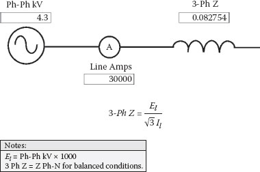
FIGURE 2.2
Amps to Z Conversion
By convention, when MVA is used to express short circuit duty, the three-phase balanced apparent power formula is used to determine current magnitudes for both balanced and unbalanced faults. Figures 2.4, 2.5, and 2.6 cover balanced three-phase conversion calculations for MVA, amps, and ohms, respectively.
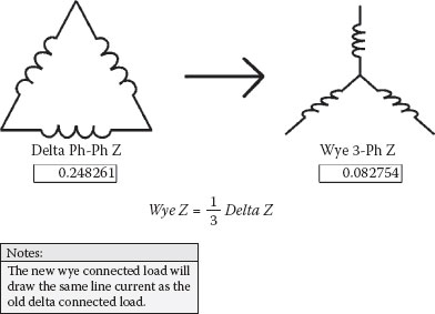
FIGURE 2.3
Delta to Wye Z
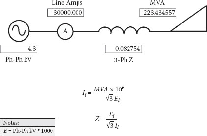
FIGURE 2.4
MVA to Amps and Z
By analyzing the foregoing figures, you will find that 30,000 amps is equal to .083 ohms, which is equal to 223 MVA. All three parameters can be used to describe the same short circuit magnitudes for 4.3 kV three-phase balanced conditions.
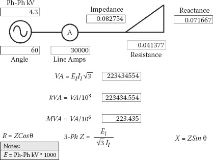
FIGURE 2.5
Amps to MVA and Z
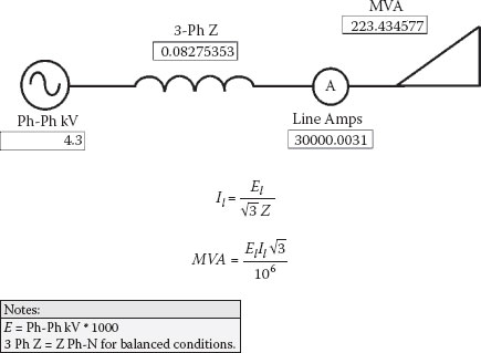
FIGURE 2.6
Z to MVA
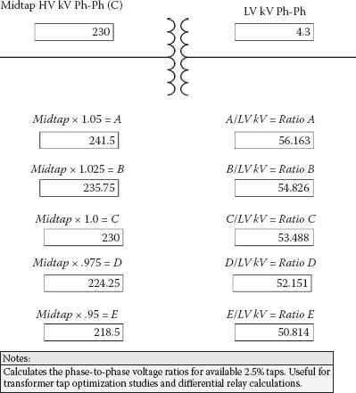
FIGURE 2.7
Transformer Winding Tap Ratios
2.2 Transformer Tap Optimization
The second phase for electrical studies usually involves optimizing transformer winding tap positions, as any changes in ratio will impact the studies.
If the annual peak primary voltage is known, an optimum tap can be selected for the transformer under study. If measured data are not available, a peak voltage of 105% of nominal can be assumed, that is, 230 times 1.05 = 241.5 kV. As presented in Figure 2.7, transformers normally have five no-load tap positions, two above mid-tap, and two below. Each step or tap change increases or reduces the mid-tap voltage ratio by 2.5%.
Although it is hard to say anything absolute about motors because there are numerous design variations, most motors will run more efficiently at higher voltages. In many cases, the motors will require less stator amps to produce the same horsepower, which reduces the corresponding watt and var losses (amps squared × R and × X, respectively). Also, operating at higher voltages provides additional margin for system low voltage conditions. The limiting factor is normally the continuous voltage rating of motor loads on the secondary side of transformers. The optimum tap setting provides the highest voltage that will not reduce the life of motors during worst-case operating conditions when the primary voltage is at its highest and the transformer load is low (minimizing the voltage drops in the source transformer and conductors).
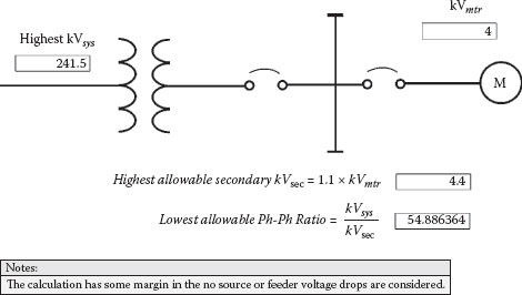
FIGURE 2.8
Transformer Winding Tap Optimization
The procedure illustrated in Figure 2.8 provides the lowest allowable phase-to-phase voltage ratio that can be applied without exceeding the continuous voltage rating of the motors. The lower the winding ratio, the higher the voltage on the secondary side. Although motors have a continuous voltage rating of 110% of nameplate, the nameplate value is normally below the nominal bus voltage; that is, 480 volt motors have nameplate ratings of 460 volts and 4 kV motors either 4 kV or 4.16 kV with a nominal bus voltage of 4.3 kV. The author prefers 4.16 kV motor nameplate values for improved operating margins or less likelihood that the 480 voltage levels will be limited by how high the 4 kV system can operate. In the case of 4 kV nameplate motors, the limitation would be 110% of 4 kV or 4.4 kV, which would be the maximum continuous voltage rating of the motors. Figure 2.8 shows a RAT-fed 4 kV bus from Figure 1.23 (in Chapter 1) with the 230 kV system at its highest voltage of 241.5 kV and a lowest allowable winding ratio of 54.866. Tap B would provide a ratio of 54.826 as indicated in Figure 2.7 and would be the optimum choice. In regard to 460 volt nameplate motors, the limitation is 110% of 460, or 506 volts.
Volts/Hz withstand curves for generators and transformers are readily available from a number of manufacturers. The curves for transformers and generators will generally have the same slope, but generators start with a lower continuous rating of 105% and transformers at 110% (same as motors). Because motor curves are not readily available, the bullets presented below were extrapolated from one of the more conservative volts/Hz curves for transformers and should reasonably represent motor withstand times as well:
• 134% = 0.1 minutes
• 131% = 0.2 minutes
• 126% = 2.0 minutes
• 120% = 5.0 minutes
• 116% = 20 minutes
• 114% = 50 minutes
• 111% = 100 minutes
Motor, generator, and transformer voltage levels are limited by the level of magnetic flux that their core iron laminations can carry without overheating. The term volts/Hz is used to account for operation at reduced frequencies that lower the impedance and increase the excitation of the core iron. At 60 Hz, the percent volts/Hz corresponds directly to the overvoltage magnitude; that is, 115% overvoltage = 115% volts/Hz.
Figure 2.9, covers the procedure for calculating the impact of operating a 4 kV nameplate motor at a reduced frequency of 58 Hz. For reference purposes, the maximum bus and potential transformer secondary voltages at 60 Hz are determined to be 4.4 kV and 125.7 volts, respectively. A base volts/Hz ratio is calculated by dividing the rated or nameplate kV by the rated frequency. An applied volts/Hz ratio is then determined by dividing the applied kV by the applied frequency. The applied volts/Hz percentage can be calculated by dividing the applied ratio by the base ratio and multiplying by 100. In this example, the motor’s maximum continuous volts/Hz rating of 110% is exceeded with a calculated percentage of 111% even though the 60 Hz maximum rated voltage of 4.4 kV is greater than the applied voltage of 4.3 kV. This is because the applied frequency of 58 Hz reduces the impedance of the stator windings, which increases the ampere turns and resulting magnetic flux in the stator core iron laminations.
The next step for performing electrical studies usually involves determining the ampere ratings and impedance data of the associated electrical conductors.
In general, smaller conductors are mostly resistive in nature. As the size of the conductor increases (geometrical mean radius, or GMR), the inductive reactance reduces slightly and the conductor resistance reduces more dramatically. The inductive reactance reduces because of the effect of annular current flow (eddy currents) in the extra conducting material near the skin effect region or boundary that produces a counter flux resulting in a lowered self-flux opposition voltage as illustrated in Figure 2.10. Somewhere around medium size, the conductor resistance will equal the inductive reactance, and larger conductors will be mostly inductive in nature.
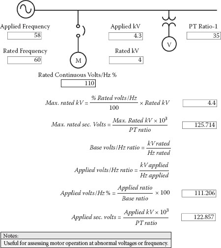
FIGURE 2.9
Motor Volts/Hz Withstands
Generally speaking, copper and aluminum bus ampacities are a function of cooling, the cross-sectional areas, and the purity of the metals used to fabricate the bus bars. The calculation in Figure 2.11 is sometimes utilized in plants for the construction of copper bus bar jumpers and allows for a 30°C rise above ambient temperatures with the calculated current flowing. This calculation is conservative and has more than ample margin because the standards for buses allow for a much greater temperature rise.
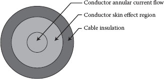
FIGURE 2.10
Conductor Radius and Inductance
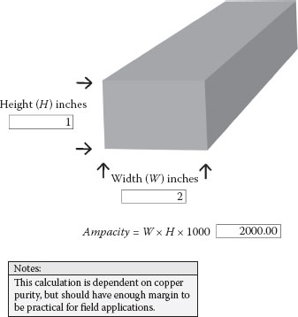
FIGURE 2.11
Copper Bus Ampacity
The manufacturer of the busway normally provides the ampacity and impedance parameters for a specific design. Figure 2.12 shows the resistance and inductive reactance values for a 500-foot run of 2000 amp low voltage copper busway (480 volt applications) manufactured by the Square D Company. The resistance value assumes a conductor temperature of 80°C.
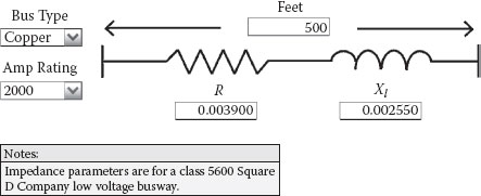
FIGURE 2.12
Low Voltage Busway
In general, cable ampere ratings are a function of the amount of copper, the temperature rating of the insulation, and the design of the raceway system. Although specific ampacity values can be obtained from the manufacturer, tables in the National Electrical Code (NEC) are commonly used to determine the ampacity for a particular design. Cable impedance data can be furnished by the manufacturer or taken directly from tables provided in IEEE Standard 141.
Figures 2.13 and 2.14 present the ampere rating and impedance parameters for a 500-foot run of 1000 kcm copper-insulated 90°C low voltage cable (480 volt applications) installed in magnetic and nonmagnetic conduit, respectively. By comparing the resistance values, it can be seen that the resistance is higher with magnetic conduit due to eddy current watt losses in the rigid conduit. Because most of the eddy current heating takes place in the conduit, the cable ampere rating is not impacted. The reactance values are also a little higher with magnetic conduit because the magnetic flux is attracted to the conduit, which results in a weaker subtractive effect from the other phases and increased self flux. Three conductors in one conduit are assumed for determining the ampacity, and a conductor temperature of 75°C is assumed for the conductor resistance values. More than three phase conductors in one conduit will require a reduced ampere rating because of the heat transfer from the other conductors; this is covered in the NEC. In somewhat balanced systems without significant harmonic content, the neutral conductor does not need to be considered in the derating. The ampacity values comply with NEC Table 310-22, and the impedance parameters are in agreement with IEEE Standard 141. The cable reactance values are higher than the busway inductive reactance shown in Figure 2.12, even though the busway spacing between phases is greater, because of the higher ampacities and geometries of the bus bars.
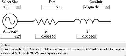
FIGURE 2.13
Low Voltage Cable in Magnetic Conduit
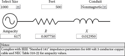
FIGURE 2.14
Low Voltage Cable in Nonmagnetic Conduit
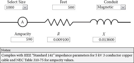
FIGURE 2.15
Medium Voltage 5 kV Cable in Magnetic Conduit
Figure 2.15 the presents the ampacity and impedance parameters for a 500-foot run of 5 kV 1000 kcm copper-insulated 90°C medium voltage cable (4 kV applications) installed in a magnetic conduit. Three conductors in one conduit are assumed for determining the ampacity and a conductor temperature of 75°C is assumed for the conductor resistance value. The ampacity value complies with NEC Table 310–75 and the impedance parameters are in agreement with IEEE Standard 141. The resistance is higher due to the conduit eddy current watt loss.
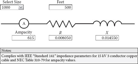
FIGURE 2.16
Medium Voltage 15 kV Cable in Nonmagnetic Conduit in Earth
Figure 2.16 provides the ampacity and impedance parameters for a 500-foot run of 15 kV 1000 kcm copper-insulated 90°C medium voltage cable installed in underground nonmagnetic conduit. Three conductors in one conduit and a soil thermal resistivity (RHO) of 90 are assumed for determining the ampacity, and a conductor temperature of 75°C is assumed for the conductor resistance value. The ampacity value complies with NEC Table 310-79, and the impedance parameters are in agreement with IEEE Standard 141. The inductance is higher than the 5 kV cable as a result of the increased spacing caused by the thicker 15 kV insulation, which overrides the magnetic conduit effect in the 4 kV cable. The ampacity is higher because the ground or earth acts as a heat sink and drains heat away from the cable.
2.3.3 Overhead Aluminum Conductor Steel Reinforced (ACSR) Cable
The ampacity and impedance values for overhead ACSR cables are provided in the Westinghouse Transmission and Distribution Reference Book and in other publications. Phase conductor spacing impacts the inductive reactance values. The magnetic self-flux that links with the conductor to cause the opposition voltage or inductive effect increases when the spacing is greater because the subtractive magnetic fluxes from the other phases have a weaker effect. If all three phase conductors could occupy exactly the same position or location, the inductive reactance would be zero because the vector sum of all three magnetic fluxes would be zero. This, of course, is not possible because the phases must be insulated from each other to prevent short circuit currents from flowing. This is illustrated in Figure 2.17 where the overlapping flux gradient from other phases subtracts from the self flux originating from each conductor. Consequently, to more accurately determine the impedance values, the spacing between phases must be known. Usually this spacing is not symmetrical, and the unbalanced spacing must first be converted to an equivalent uniform spacing or geometrical mean distance (GMD) before the symmetrical spacing parameters provided in the references can be applied. Figure 2.18 illustrates an equivalent uniform spacing of 3.1 feet for three-phase conductors that are separated by 2, 3, and 5 feet, respectively.
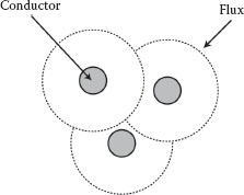
FIGURE 2.17
Spacing Impact on Inductance
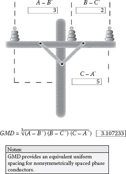
FIGURE 2.18
Equivalent Symmetrical Conductor Spacing
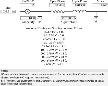
FIGURE 2.19
18 kV 1033.5 ACSR 3-Foot Spacing
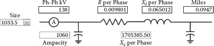
FIGURE 2.20
138 kV 1033.5 ACSR 12-Foot Spacing
Figures 2.19 and 2.20 show the impedance parameters for 18 kV (3-foot) conductor spacing and 138 kV (12-foot) conductor spacing, respectively. The actual spacing may differ significantly based on local weather and other environmental conditions; distance between spans; and concerns over galloping conductors, pole or tower support details, and margins preferred by the local utility. However, the effects are linear, and the actual reactance values can be extrapolated from reactance values associated with greater and lesser spacing. Although shown in miles, the line distance is equivalent to 500 feet for comparison to the other conductors already discussed. Comparing Figures 2.19 and 2.20, you will find that the resistance and ampacity values are the same, but the inductive and capacitive reactance values are higher for the 138 kV overhead cables due to the increased spacing between conductors. As mentioned before, increasing the spacing weakens the subtractive flux from the other phases which increases the self flux and inductance. The capacitive reactance increases because the distance between plates increases which reduces the microfarad value.
At this point in the chapter, we have addressed the preliminary data gathering, conversions, transformer tap optimization, and conductor parameters required for studies and can now proceed with the actual procedures for voltage, power transfer, and short circuit calculations. Calculations require only a precision that is practical for the particular application. Most calculations do not consider the exciting current associated with transformers or stray capacitance. Some calculations consider only the reactive and not the resistive components. Many procedures assume nominal magnitudes for voltages and other parameters and not actual values that may be in play prior to or during electrical system faults and disturbances. However, experience has shown that the calculation methods presented in this chapter and throughout the book have enough precision to be practical for the intended applications.
Figure 2.21 provides a procedure for calculating bus voltage drops for balanced loads. First, the circuit MVA is converted to amps using the standard three-phase power formula. Next the impedance parameters (R and X) for the total circuit are calculated. Then the portion of R and X that is associated with the load only is determined. Finally, the sum of the resistive and reactive voltage drops at the load are calculated and then multiplied by the square root of 3 or 1.732 for conversion from a phase-to-neutral to a phase-to-phase voltage magnitude. In this example, because of the source impedance, the voltage at the bus is reduced from 4.3 kV to 3.8 kV. The power factor or angle will impact the results of the calculation.
Figure 2.22 provides a similar procedure for calculating line voltage drops for balanced loads. First the total circuit R and X is determined. Then the load R and X is derived. Finally, the sum of the resistive and reactive voltage drops at the load are calculated and then multiplied by the square root of 3 or 1.732 for conversion from a phase-to-neutral to a phase-to-phase voltage magnitude. As you can see, the voltage at the load is reduced from 4.3 kV to 3.95 kV due to the source and cable impedance.
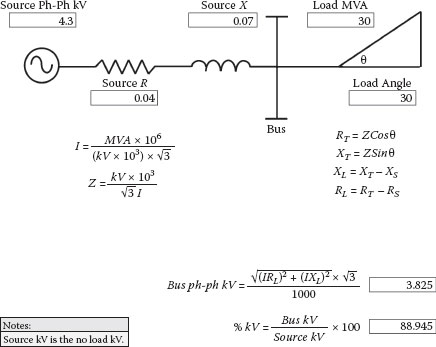
FIGURE 2.21
Bus Voltage Drop
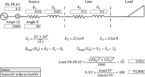
FIGURE 2.22
Line Voltage Drop
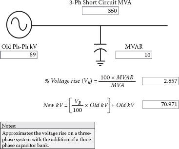
FIGURE 2.23
Capacitive Voltage Rise
Figure 2.23 covers how to approximate the effect that three-phase balanced capacitance has on voltage levels. If the total circuit capacitance in megavars (MVAR) times 100 is divided by the short circuit duty in MVA, the result will yield the percent voltage rise of the circuit. The voltage rise could be caused by installed capacitor banks or by the capacitance of long transmission lines that are lightly loaded. In this example, the addition of a 10 MVAR bank will increase the voltage from 69 to almost 71 kV.
Figure 2.24 discloses how to calculate the unfaulted phase-to-phase voltages if the faulted phase-to-phase voltage is known. This is useful for unbalanced voltage studies and for testing some phase-to-phase impedance relay elements. In this case, if the C-B voltage is reduced to 50 kV, the unfaulted phase-to-phase voltages will be reduced to 201 kV.
2.6 Power Transfer Calculations
Figure 2.25 deals with the basic power transfer equations for three-phase watts and vars caused by voltage and angular differences or delta (power angle) between two different points on an electrical system and the limiting affects of the total circuit inductive reactance ohms. Angle in this case refers to angular differences between the voltage on bus 1 versus the voltage on bus 2. If phase-to-phase voltages are used in the equations, the calculations yield three-phase watt and var magnitudes that will flow from one point to the other. In general, watts will flow from the leading to the lagging angle and vars will flow from the higher to the lower voltage system. In this example, a 10-degree angular delta between bus 1 and bus 2 causes 18.9 MW and 0.8 MVAR to flow from bus 1 to bus 2 when the buses are operated in parallel.
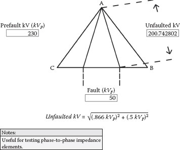
FIGURE 2.24
Collapsing Delta
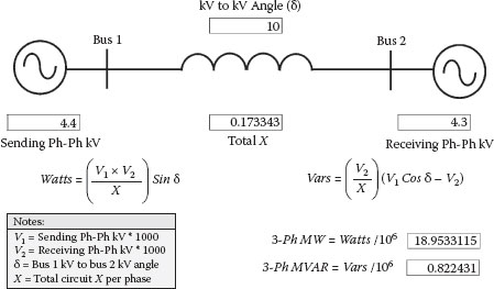
FIGURE 2.25
Power Transfer Equations
Figure 2.26 illustrates a two-generator system with identical turbines and generators. The right triangle in the first quadrant represents a typical system load that is resistive and inductive and series in nature. The current is the reference, and the voltage phasor falls into alignment with the hypotenuse or VA of the right triangle. If equal steam flows through each turbine and the field or excitation currents are the same, each generator would provide one-half the watt and one-half the var requirement of the system load. If the generator governors are on manual and steam flow is increased for machine A, it would feed a greater portion of the watt requirement, and the system frequency would increase if machine B did not back down. The increased steam flow in machine A would cause its power angle to increase (in the leading direction), which would put it in advance of machine B, allowing it to feed a greater portion of the load. If the generator automatic voltage regulators (AVR) are also on manual and excitation or field current is increased for machine A, it would feed a greater portion of the var requirement and the system voltage would increase if machine B did not back down on excitation. This is referred to as boost vars, and if the power factor was measured for generator A, it would show that the current was lagging the voltage by a greater amount. If the excitation for A is increased high enough, the total system var requirement would be fed by A and generator B would be at unity power factor. If the excitation for A is increased beyond that point, B would become a var load for A and the current in B would lead the voltage, resulting in buck vars. In this case, the right triangle for B would be inverted and shown in the fourth quadrant.
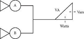
FIGURE 2.26
Two-Generator System
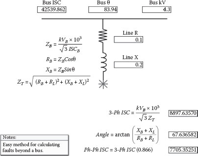
FIGURE 2.27
Short Circuit: No Transformer
2.8 Ohmic Short Circuit Calculations
Short circuit calculations that do not involve transformation can easily be performed using ohmic values.
Figure 2.27 covers how three-phase short circuit current at the end of a line impedance can easily be determined if the short circuit duty at the source bus is known. The bus short circuit current is converted to R and X values that can be added to the line R and X, and then the total current at the end of the line can be determined by using three-phase Ohm’s Law. The phase-to-phase short circuit current is normally equal to 86.6% of the three-phase value because the ratio of three-phase ohms to phase-to-phase ohms equals 1.732/2 or .866. three-phase ohms = (phase-to-phase E/1.732 I), and phase-to-phase ohms = (phase-to-phase E/2 I) because the return impedance of the second phase needs to be considered.
When two sources are operated in parallel, the short circuit contribution from each source needs to be added together to determine the total short circuit current. If the angles are the same, the new total current will simply be the algebraic sum of the two currents. However, if there are angular differences, a conductance, susceptance, and admittance method for solving parallel impedances can be applied to determine the total magnitude of the combined currents. Figure 2.28 presents a method of resolving the total short circuit current from two sources that have angular differences. Figure 2.29 shows the reverse process of subtracting out or removing a source with angular differences from the total value. In regard to generating stations, these calculations are particularly useful for determining high voltage switchyard short circuit currents when generating units are on and off line. They are also useful for determining the combined short circuit currents of the generator and GSUT at the UAT primary terminals.
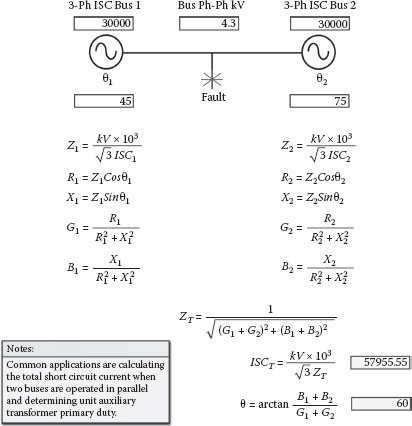
FIGURE 2.28
Short Circuit: Parallel Sources
Whenever transformers are involved in a study, it is normally easier to use a percentage or per-unit approach for resolving problems because of the different voltages involved in the study. Because ohmic values depend on which side of the transformer (primary or secondary) you are looking at, transformer impedances are almost always expressed as a percentage. The per-unit value is simply the percentage divided by 100; for example, a 7% impedance transformer would have a per-unit impedance of .07. Because a transformer’s primary MVA is equal to its secondary MVA, a percentage or per-unit system can be applied as long as the base values chosen for MVA, voltages, impedances, and currents are consistent. The base values are normally selected for convenience to be in agreement with apparatus nameplate values or with other data or studies that were previously performed. During the course of studies, it is often necessary to adjust values to a different base to be consistent with other data or to convert to other forms that are more convenient.
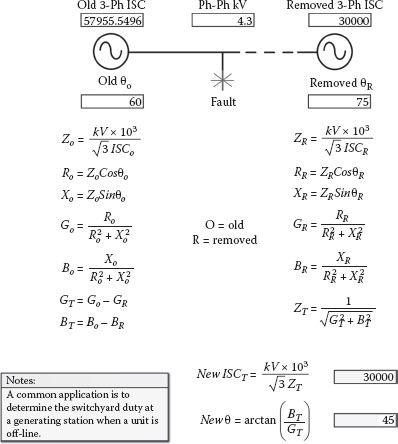
FIGURE 2.29
Short Circuit: Removing Parallel Sources
Although it is not always obvious, the basic formulas presented in Chapter 1 still apply when using the per-unit system. One complication is that 1.0 per unit could represent full load amps or some other parameter and because ones can easily drop out of formulas, the expressions may no longer be presented in a manner that is familiar to the reader. For example:
• Per unit (pu) amps = pu volts/pu Z
• Amps = pu amps × base amps; or shortcut method:
• Amps = base amps/pu Z
The percent or per-unit impedance of transformers often needs to be adjusted for applied winding taps and actual applied voltages that are different than the nameplate base values. The nameplate will show the %Z at a specified MVA and winding tap. Normally, it would be specified at the OA (oil and air) or lower MVA rating and for the mid-tap winding voltage. If the applied voltage is different or the selected tap is different, the %Z self-cooled rating is usually adjusted or corrected for the differences. Figure 2.30 is used to adjust or correct a transformer’s base per-unit impedance to a different winding tap. Figure 2.31 is the same calculation used again to convert the transformer’s tap corrected base per-unit impedance to the actual applied or system voltage of 14 kV. Figure 2.32 combines both calculations into a single expression that corrects for both winding tap and applied voltage differences.
A transformer’s infinite bus (unlimited supply) three-phase short circuit current can be calculated by dividing its rated three-phase current by its per-unit impedance, as shown in Figure 2.33. Using the primary kV base current provides the primary current for a secondary fault, and using the secondary kV base current provides the secondary current for the same fault. Figure 2.32 represents the transformer displayed in Figure 2.33; the calculation yields the infinite source three-phase secondary short circuit current on the 14 kV side and is probably within 90% or more of the actual value for faults near the secondary bushings or terminals. However, standard practice is to complete a more refined calculation that includes the source and line impedance to the short circuit location.
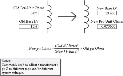
FIGURE 2.30
Transformer Winding Tap Correction
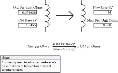
FIGURE 2.31
Transformer Applied Voltage Correction
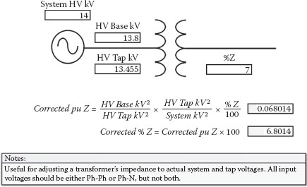
FIGURE 2.32
Transformer Tap and Applied Voltage Correction

FIGURE 2.33
Per-Unit Z to Amps
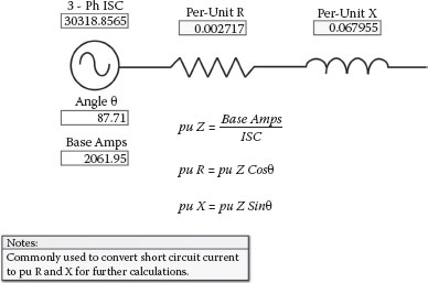
FIGURE 2.34
Amps to Per-Unit R and X
2.9.4 Amps to Per-Unit R and X
Figure 2.34 illustrates how to calculate the per-unit R and X angle if the short circuit angle is known, and Figure 2.35 covers how to determine the balanced three-phase short circuit current if the per-unit R and X are given.
Occasionally, MVA base values need to be adjusted to accommodate different apparatus or data from another study. Figure 2.36 shows how to adjust per-unit ohms from a 50 to a 100 MVA base. The impedance does not need to be corrected for single-phase transformers that are used in three-phase banks. Although the combined MVA is higher, the base current does not change and “three-phase ohms” equal “phase-neutral ohms.” A 7% single-phase 10 MVA transformer also has a 7% impedance when used in a three-phase 30 MVA bank.
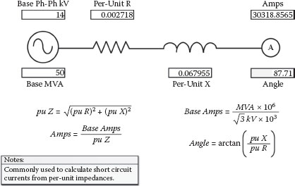
FIGURE 2.35
Per-Unit R and X to Amps
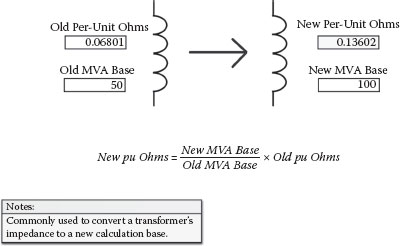
FIGURE 2.36
New MVA Base
At some point in your study, per-unit ohms may need to be converted to actual ohms for protective relay or other applications. This can be accomplished using the formula presented in Figure 2.37. The inverse calculation is shown in Figure 2.38.
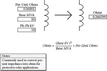
FIGURE 2.37
Per Unit to Ohms
Converting amps to per-unit Z is useful for some applications, as shown in Figure 2.39; for example, dividing a motor’s full load amps (FLA) by the locked rotor current (LRA) provides the per-unit impedance of the motor.
2.10 Per-Unit Short Circuit Calculations
2.10.1 Transformer Short Circuits
Figures 2.40, 2.41, and 2.42 provide procedures for calculating short circuit currents for the three most common transformer configurations. By comparing the procedures in all three figures, it can be seen that they are the same for determining secondary three-phase and phase-to-phase short circuit currents and the results are the same. Additionally, the primary currents for secondary three-phase faults are the same in all cases. However, the wye-delta and delta-wye winding configurations cause the current to increase in one of the primary phases for secondary phase-to-phase faults. The delta-wye grounded transformer can also deliver ground fault current.
2.10.2 Transformer Three-Phase and Phase-to-Phase Fault Procedures
Let’s start with the delta-delta transformer in Figure 2.40 because the short circuit currents are easier to calculate. First, an MVA base is selected; using the transformer MVA as the base avoids additional conversions. Next, the source short circuit current is converted to R and X and then to per-unit values. The transformer percent impedance is also converted to per-unit R and X values using the X/R ratio, and finally the line R and X is converted to per-unit R and X values. The three-phase secondary fault current is the secondary base current divided by the total per-unit impedance and the angle is the arc-tangent of the per-unit X/R ratio. Dividing the secondary short circuit current by the phase-to-phase ratio will yield the primary current. The secondary phase-to-phase fault current magnitude is 86.6% of the three-phase value and in this configuration, the secondary current divided by the ratio yields the primary current. Figure 2.40 also provides typical X/R ratios if specific transformer X/R ratios are not available.
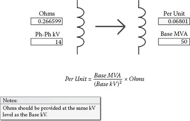
FIGURE 2.38
Ohms to Per Unit
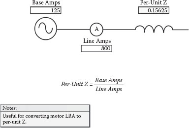
FIGURE 2.39
Amps to Per-Unit Z
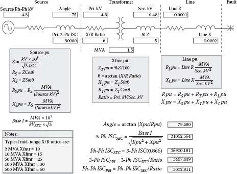
FIGURE 2.40
Delta-Delta Transformer Short Circuit
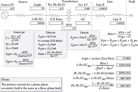
FIGURE 2.41
Wye-Delta Transformer Short Circuit
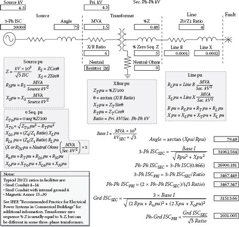
FIGURE 2.42
Delta-Wye Transformer Short Circuit
For the wye-delta and the delta wye transformers in Figures 2.41 and 2.42, the calculating procedures are identical with Figure 2.40 except for primary currents for phase-to-phase secondary faults. In both cases, one of the primary phases sees it the same as a three-phase 100% fault even though it is really an 86.6% phase-to-phase fault. The delta-wye grounded configuration can also deliver ground fault current.
Let’s take a look at the phase-to-phase current flow for the delta-wye transformer in Figure 2.42 first because it is simpler. Figure 2.43 illustrates current flow for an A-B fault. As you can see, B phase has a greater primary current due to the contribution from the other two phases. Figure 2.44 shows the phasor relationships.
Figure 2.45 illustrates the current flow for the wye-delta transformer in Figure 2.41 for an A-B secondary fault. The current flow in this case is much more complicated than the delta-wye transformer configuration. In addition to the A-B winding, the B-C winding in series with the C-A winding is in parallel with the fault and also provides fault current to the A-B fault, which increases the primary current in A phase.
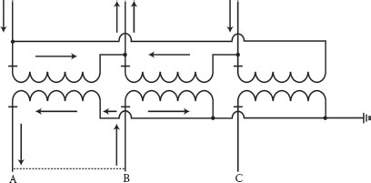
FIGURE 2.43
Delta-Wye Transformer Phase-to-Phase Fault Currents
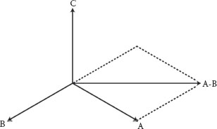
FIGURE 2.44
Delta-Wye Transformer Phase-to-Phase Phasors
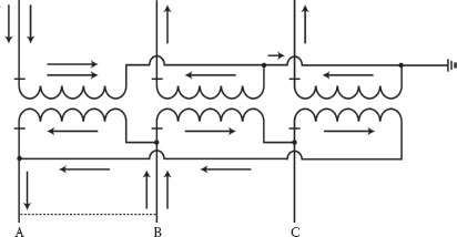
FIGURE 2.45
Wye-Delta Transformer Phase-to-Phase Fault Currents
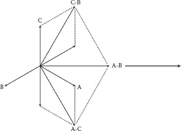
FIGURE 2.46
Wye-Delta Transformer Phase-to-Phase Phasors
Figure 2.46 illustrates the phasor relationships. The B-C and C-A vectors are reversed because current flows in each secondary winding are in on polarity instead of out on polarity. Two A-B vectors are shown, one for each winding configuration that feeds the fault.
Calculating ground faults and analyzing unbalanced conditions for three-phase systems can be quite complex. In 1918, Dr. C. L. Fortescue presented a paper at an American Institute of Electrical Engineers (AIEE) convention in Atlantic City, New Jersey, on a method for analyzing three-phase systems using positive, negative, and zero sequence phasors (symmetrical components). Positive sequence (1) represents normal balanced conditions and rotation; negative sequence (2) represents unbalanced currents in the armature or stators of rotating electrical apparatus that produce a reverse rotation current in the rotors or fields of generators and motors; and zero sequence (0) represents ground fault currents without rotation. Consequently, many in the industry will refer to balanced events as positive phase sequence, phase-to-phase events as negative phase sequence, and ground faults as zero phase sequence. Although the foregoing is really an oversimplification of symmetrical components, ground fault currents through delta-wye transformers can be readily calculated with a procedure that utilizes positive, negative, and zero sequence impedances. Figure 2.47 illustrates the sequence impedances (for simplification, it does not show the resistance) that will be utilized. Figure 2.48, for illustrative purposes, is mathematically the same, but applies the ground return path impedance to each sequence leg, negating the need to multiply the ground return path impedance by 3.
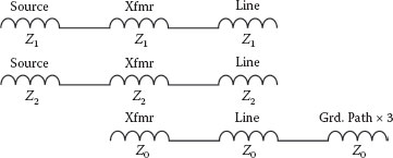
FIGURE 2.47
Normal Delta-Wye Ground Fault Sequence Impedances
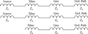
FIGURE 2.48
Equivalent Delta-Wye Ground Fault Sequence Impedances
2.10.4 Transformer Ground Fault Procedure
Referring to Figures 2.42 and 2.47, basically the base current is multiplied by 3 and then divided by the sum of the positive, negative, and zero sequence per-unit impedances. The positive sequence per-unit impedances are derived from the source impedance, percent impedance of the transformer, and the line ohmic values to the point of the fault. The positive and negative sequence magnitudes are considered equal to each other, and doubling the positive sequence impedances will account for both in the equation. The zero sequence impedance includes the transformer zero sequence %Z (usually considered the same as the %Z of the transformer but can be lower in three-phase core form transformers), line and ground return path impedances and any limiting impedance in the neutral. Because the base current is multiplied by 3, any impedance introduced in the transformer neutral and in the ground return path has to be multiplied by 3 to balance out the equation.
As you can see in Figure 2.42, the ground fault magnitude exceeds the three-phase fault value because the zero sequence impedance does not include the source impedance. However, the zero sequence impedance increases faster than the positive sequence impedance as the distance from the transformer to the ground fault location increases; therefore, the three-phase short circuit current often exceeds the phase-to-ground fault current at the secondary side circuit breaker. Transformers and generators are generally not designed to handle large close in ground fault currents that are above the three-phase value; consequently, some transformers are equipped with neutral reactors to limit the close in ground fault current, and generators are normally high impedance grounded to limit the ground current. Figure 2.42 also provides typical Z0/Z1 ratios for commercial and industrial facilities. The positive sequence impedances for cables and busways can be multiplied by a Z0/Z1 ratio to estimate the impedance for the line plus the ground return path (does not include transformer neutral-to-ground impedance). Because, the overall Z0/Z1 ratio can range from as little as 1 to as much as 50, precisely estimating the ratio is not practical because of the many variables in ground current return paths. Because of this, worst-case conditions are often assumed when making ground fault calculations for short circuit duty considerations. The suggested Z0/Z1 ratio of 4 assumes that the ground return path impedance equals the line impedance to the point of the fault and is the more conservative calculation.
Figure 2.49 shows a representation of the line impedance as 1 ohm and the ground return path as 1 ohm times 3. The overall zero sequence impedance for the line plus the return path equals 3 plus 1, or 4. Accordingly, in this case, the Z0/Z1 ratio equals 4. For Z0/Z1 ratios greater than 4, much of the circuit impedance is in the line itself due to the increased spacing between the line and the return path. In analyzing the Z0/Z1 ratios presented in Figure 2.42, the lowest Z0/Z1 ratio of 4 is assigned when a ground conductor is provided in the same conduit as the line conductors, reducing the spacing between the line and ground return path and the associated self flux and inductive reactance of each conductor.
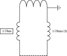
FIGURE 2.49
Z0/Z1 Ratio
2.10.5 Alternative Ground Fault Procedure
As a matter of interest, delta-wye ground fault current can also be determined without resorting to sequence impedances by applying more conventional methods without major difficulty for applications that do not involve parallel sources on the wye side. It is really a relatively simple circuit with current flows in only one of the three single-phase transformers that make up a three-phase bank. It can also be debated that this method is simpler, has fewer steps, and relies on conventional theory instead of a sequence impedance procedure that is contrary to actual basic theory. The sequence impedance method (which provides an equal result) advocates 3V0 and 3I0, which can be calculated but do not really exist, suggests that the ground fault current is higher at the transformer because the source impedance is not considered in the zero sequence path (which is not the real reason), and that the zero sequence impedance increases rapidly because it is multiplied by 3 (which is also not the real reason). Figure 2.50 illustrates the same delta-wye grounded transformer with an identical C-phase secondary ground fault, but in this case, the actual current paths and impedances will be utilized.
As you can see by the current flow, the ground fault looks like a phase-to-phase fault to the source. Consequently, the phase source impedance is multiplied by 2 to consider the impedance from two different phases. Twice the source impedance is then reflected to the secondary or 480 side (calculation for step-down transformer only). The transformer ohms are also determined on the 480 volt side, and the ground return path impedance is assumed to equal the line impedance (Z0/Z1 ratio of 4). Therefore, doubling the line impedance also accounts for the return path impedance. Finally, the total neutral or ground current can now be determined by dividing the phase-to-neutral voltage by the total impedance (including the neutral-to-ground impedance if applicable). If you compare the ground fault current magnitudes in Figure 2.50 to those in Figure 2.42, you will find that they are identical. The ground fault current exceeds the three-phase value near the transformer because the ratio is higher (higher secondary current) because phase-to-neutral instead of phase-to-phase voltages are utilized in the calculation. The ground fault impedance increases faster than the three-phase impedance because the three-phase calculation does not need to consider the return path impedance. The ground fault angle can now easily be determined by the arc-tangent of the X/R ratio.
2.10.6 Generator Three-Phase Short Circuits
Figure 2.51 presents the three 3-phase short circuit levels for generators. Basically, the highest level of current occurs during the first few cycles and is calculated by dividing the base current by the direct axis saturated subtransient per-unit reactance or impedance. This is the reactance that is typically applied for short circuit studies and represents the flux magnitude prior to the fault. The direct axis saturated subtransient reactance (Xd”) is used when generators are at rated voltage (slightly saturated) prior to the fault and the pole faces are more directly aligned with load currents. A short circuit angle of 90 degrees lagging is often assumed for large generators, but if the X/R ratio is known, a more refined angle can be determined. The mid-level of fault current is calculated by dividing the base current by the direct axis saturated transient per-unit reactance (Xd’). This level of fault current typically lasts for tenths of seconds. The final level is determined by dividing the base current by the direct axis synchronous per-unit reactance (Xd). Please note that this level of current is normally well below the full load ampere rating of the machine; consequently, conventional overcurrent relays (without voltage restraint or control) cannot isolate generators from short circuits if they are set with time delay to coordinate with downstream devices. The foregoing current decrements are basically caused by the inability of excitation systems to overcome the internal voltage drops and subtractive magnetic flux (armature reaction) that develop during large inductive reactive current flow in the stator windings. The synchronous reactance is also used to determine voltage drops in operating synchronous generators, and both the armature reaction and the inductive reactance are included in the Xd value. As with transformers, the initial phase-to-phase fault current for practical purposes is normally 86.6% of the three-phase subtransient value. Technically, double the negative phase sequence reactance should be used for the phase-phase calculation, but any differences are usually negligible.
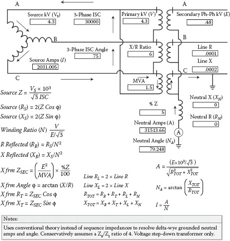
FIGURE 2.50
Alternative Ground Fault Calculation
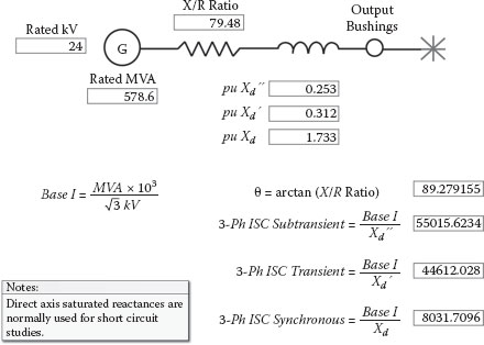
FIGURE 2.51
Generator Short Circuit
2.10.7 Generator De-Excitation
The fault current decrement is determined by the excitation system and the trapped magnetic flux in the core iron and the subtransient, transient, and synchronous reactances for bolted or low impedance faults. If the fault impedances are higher, the decrement will take longer. This is a particular problem for short circuits on the secondary side of UATs on units that are not equipped with generator bus breakers. The UAT capacity (5% to 8%) is so small (high impedance) in relationship to the generator, that the generator continues to feed fault current after electrical isolation and the tripping of the prime mover.
Two pole generators generally decay faster than four pole machines. There are a couple of commonly used methods to reduce excitation current and trapped magnetic flux in both machines. Figure 2.52 illustrates a direct field breaker; when the unit is tripped off-line, a resistor (often equal to the DC field ohms) is inserted across the field as the main contacts are in the process of opening to discharge the field current and trapped flux more rapidly. As generator designs grew larger in size during the 1970s, the DC excitation current became higher and direct field breakers became more expensive. Somewhere around 300 MVA and larger, it became more economical to indirectly interrupt the excitation power supply instead of the field current directly. Improved designs had de-excitation circuitry that reversed polarity on the field for faster fault current decrements. Although de-excitation circuitry was generally an option, it is often not used and difficult to apply on cross-compound units (HP and LP turbogenerators operated in parallel). Both the direct field breaker and the de-excitation circuitry reduce the UAT secondary fault current to approximately zero in around 4 seconds depending on design details. Because transformers are generally built to withstand the electromechanical forces from fault currents for only 2.0 seconds, it is not unusual to fail auxiliary transformers from through fault conditions that trip almost instantaneously from transformer differential protection. During the 1980s, a large coal plant in Nevada that was not equipped with direct field breakers or de-excitation circuitry developed a short circuit in the busway between the UAT and secondary circuit breaker. Although the UAT differential relays actuated and tripped the unit in around 6 cycles, the cross-compound generators continued to feed fault current to the short circuited secondary bus for 42 seconds during coast down. Obviously, the transformer required replacement after the event even though the fault was external and unit tripping was almost instantaneous.
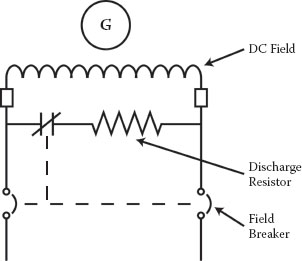
FIGURE 2.52
Direct DC Field Breaker
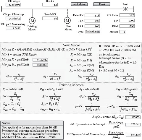
FIGURE 2.53
Motor Symmetrical Short Circuit Contributions
Motors can contribute current to short circuits for a few cycles because of the rotating inertia and trapped magnetic flux in the core iron. Normally, motor contribution does not need to be considered when coordinating overcurrent relays because of the rapid decay. However, it may need to be considered when analyzing instantaneous protection elements. It definitely needs to be included when calculating the interrupting and momentary short circuit current capabilities of switchgear circuit breakers. This will be discussed in more detail under circuit breaker duty calculations in Chapter 5. Figure 2.53 shows a procedure for calculating the symmetrical portion of motor current contribution for circuit breaker interrupting and momentary ratings and can also be used for other studies concerned with motor symmetrical current contribution. In the example, only one motor is considered in the calculation, and the old motor values represent that motor in advance of entering new data for the next motor. The motor per-unit Z is determined by dividing the motor full load amps by the maximum locked rotor amps. This value is then converted to a common MVA base, which should be equal to or greater in magnitude than the largest motor on the bus. Because the motor nameplate voltage is lower than the source bus voltage, the motor per-unit impedance also needs to be corrected to the bus voltage magnitude. Depending on the type of motor (synchronous or induction), horsepower, and RPM, different multiplication factors are applied to increase the motor per-unit impedances for interrupting and momentary symmetrical contributions, respectively, to account for current decrements during protective relay and circuit breaker operating times or cycles and specific motor design details.
The motor per-unit impedance is then added to other motors previously calculated using the conductance, susceptance, and admittance method of deriving parallel impedances. The total symmetrical interrupting and momentary current contributions for all motors on the bus can then be determined by dividing the base amps by the total interrupting and momentary per-unit impedances, respectively. Cable impedance is usually considered negligible for medium voltage motors but is normally considered for low voltage motors. For low voltage motors below 50 HP, usually the contribution is assumed to be 4 times full load amps, or 0.25 per unit.
Baker, Thomas, EE Helper Power Engineering Software Program, Laguna Niguel, CA: Sumatron, Inc., 2002.
Electric Power Research Institute, Power Plant Electrical Reference Series, Vols. 1–16, Palo Alto, CA, 1987.
General Electric Corporation, ST Generator Seminar, Vols. 1 & 2, Schenectady, NY, 1984.
IEEE, Recommended Practice for Electric Power Systems in Commercial Buildings, Piscataway, NJ, 1974.
National Fire Prevention Association, National Electrical Code, Qunicy, MA, 2002.
Stevenson, William D., Jr., Elements of Power System Analysis, New York: McGraw-Hill, 1975.
Westinghouse Electric Corporation, Applied Protective Relaying, Newark, NJ: Silent Sentinels, 1976.
Westinghouse Electric Corporation, Electrical Transmission and Distribution Reference Book, East Pittsburgh, PA, 1964.