
3.6
SPREAD OPTIONS

Purpose
This chapter illustrates some of the problems that complicate option pricing in the real world. The previous chapter described how relatively simple, well-behaved options are priced. This chapter expands that discussion by adding in various complications. Although this chapter focuses on spread options, similar issues commonly complicate other types of exotic options.
Summary
A specific type of option—a spread option—is especially common in the energy market. Spread options are used to price a large variety of physical energy deals. With these options, the owner of the option benefits when the difference between two prices is above a certain level. This is like a normal option except with two asset prices. Spread options cannot be exactly priced with standard option pricing formulas, but they can be closely approximated.
Key Topics
• Spread options are exotic options. An exotic option is any option that can’t be constructed out of simpler put and call options.
• Kirk’s approximation is a commonly used way to modify a Black Scholes formula to value a spread option.
A specific type of option—a spread option—is especially common in the energy market. Spread options are used to price a large variety of physical energy deals. With these options, the owner of the option benefits when the difference between two prices is above a certain level. This is like a normal option except with two asset prices. Alternately, this is like an option with a variable strike price. A spread option has a payoff similar to a standard option except that it has more than one underlying asset (Figure 3.6.1).

Figure 3.6.1 Spread option call payoff
The prevalence of spread options in energy deals is a result of the way the energy market operates—there is a focus on moving energy from one location to another, storing it for sale at a later point, and converting it from one form to another. The profitability of doing these actions depends upon the spread between two prices compared to the cost of doing the conversion—the price here versus the price there compared to transportation costs, the price now versus the price later compared to storage costs, and the price of fuel versus the price of electricity compared to conversion costs.
Any option that can’t be replicated with standard put or call options is considered an exotic option. In contrast, the more typical put and call options are considered vanilla options. One primary difference between an exotic option, like a spread option, and less complicated options is the assumptions used to model their prices. Exotic options formulas typically include more variables than standard option formulas and sometimes those variables might not work exactly the same way.
In the case of spread options, there are typically two underlying assets—a final product and an initial product. Typically, the prices between these two assets are correlated, and this relationship determines the value of these options. There often isn’t a good way to estimate this correlation either—historical data may be misleading, and there isn’t usually a liquid enough market to determine the correlations being used by other people in the market.
Because of correlation’s effect on the price of spread options, and the difficulty in estimating it, correlation requires a lot of scrutiny. Managing the risk of a spread options portfolio requires building an infrastructure to examine correlations between products. Incorrectly estimating correlation is the single easiest way to mess up this type of option valuation. Moreover, correlation isn’t just important when a spread option trade is initiated—it needs to be monitored over the entire life of the trade.
Modeling a Spread
There is a fundamental difference between spreads and the prices of individual assets. The most common approximation of asset prices (never dropping below zero, but being able to increase much more) doesn’t describe a spread very well. Although that assumption works for something like a commodity where prices are almost never zero or negative, it doesn’t work for a spread between two prices. Spreads between two prices can be zero or negative fairly often. Other standard measures, like the concept of a percent return, don’t work either. It is impossible to calculate a percent return on something that starts at a zero price—the calculation would result in a division by zero error.
There are substantial differences between the statistical distribution commonly used to model spreads, a normal distribution, and the one used to model asset prices, a lognormal distribution (Figure 3.6.2). To get around this issue, many spread option models are the ratio of the two prices. The ratio looks a bit more like a lognormal distribution. For example, it tends not to be negative.

Figure 3.6.2 Normal and lognormal distributions
Another fundamental assumption in a model is how the spread is likely to behave in the future. For example, a coin flip has a 50-50 chance of coming up heads no matter what has occurred in the past. Not all distributions work in the same way. Some series have a distinct trend, and others tend to come back to a central trend (Figure 3.6.3).
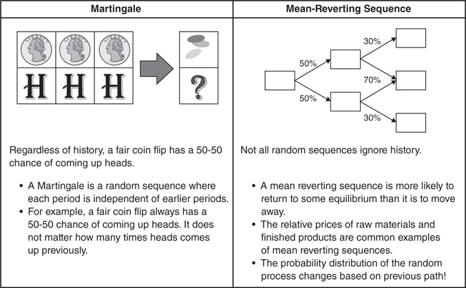
Figure 3.6.3 Mean reverting or Martingale
Spreads might fall into either category. Any time there is a conversion relationship possible between the two assets, the spread will often oscillate around the cost of conversion. For example, a crack spread relates the price of crude oil to something made out of crude oil (like gasoline). The spread between the prices of crude oil and gasoline are linked by the ability to convert crude oil into gasoline. These prices might be driven apart temporarily by short-term supply and demand issues. However, over the long run, competition between refineries is going to bring prices together again.
Prices and Correlation Estimates
Another major complication in spread options is determining the actual relationship between two assets by looking at market data. Estimating the correlation between asset prices can be especially difficult in the energy markets. One reason is that prices are often not available. Another reason is that when prices are available, they are often spot prices, which are more volatile (and less correlated) than forward prices.
When asset prices are volatile, the spread is more likely to be wide. However, when two assets are highly correlated, they behave almost like the same asset. As a result, highly correlated assets have a narrow spread (Figure 3.6.4).
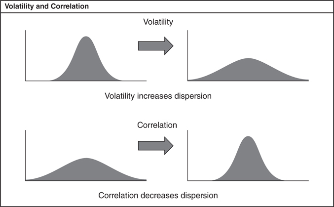
Figure 3.6.4 Volatility and correlation
This is a big deal because dispersion has a direct impact on option profitability. An option buyer will benefit from a wide range of possible spreads because an unusual spread will never result in a loss. In reverse, an option seller would benefit from a tight dispersion of possible spreads since outlying results hurt them—they will never make more than the premium, but their losses are unbounded. If either side estimates the correlation between the assets incorrectly, they will consistently lose money to someone who does a better job estimating correlations.
What Does an Actual Spread Look Like?
Modeling spreads is not just a mathematical exercise. Behind the models, options pricing ultimately needs to capture some type of actual behavior. It is often less important to understand the mathematics behind an option model than it is to understand the approximations of the real world that are being incorporated into a model.
Spread options are a great example of the importance of looking at data. One type of spread is a spark spread—the difference between the price of electricity and a fuel, natural gas. It is possible to burn natural gas to produce electricity. This is how power plants make a profit. A power plant essentially has an option to burn fuel and produce electricity.
The operational efficiency of power plants can be approximated by comparing the price of electricity to the price of fuel in the region. For example, in one area of the Mid-Atlantic powergrid, PJM-West, during the period January 2000 to June 2002, on average, it took 9.5 MMBtus of natural gas to equal the cost of 1 megawatt hour of electricity.
Looking at the price of natural gas and peak electrical power (Figure 3.6.5), the two prices are obviously correlated. The spread in prices (assuming the typical conversion of 9.5 MMBtus gas per megawatt hour of power), oscillates around zero. Sometimes the spread is positive, other times it is negative. Graphs of spot prices and the spark spread can be seen in Figure 3.6.5.

Figure 3.6.5 Historical prices
From a distribution standpoint, although there was a major outlier in prices during August 2001, the spread is clearly distributed around zero. The price of power in August 2001 was much higher than would be predicted by the cost of fuel alone. This isn’t especially surprising, since power prices often spike in the summer. As a result, it is probably a mistake to assume that the outlier is being caused by bad data. Graphing the frequency of each spread price, a normal distribution (shown overlaid in Figure 3.6.6) seems like a reasonable approximation of reality except for the huge outlier.

Figure 3.6.6 Modeling the distribution of a spread
Another issue that is clouding the predictive ability of this distribution is that the demand for power changes throughout the course of the year. A low demand for power during the spring and fall causes only the most efficient generators to run and keeps the spark spread low. In the winter and summer, an increased demand for power allows less efficient power plants to operate and drives up prices. On the hottest days, power prices can spike if the least efficient power plants have to be activated. A more realistic estimate of prices would incorporate a separate distribution for each season.
If more outliers like the August 2001 outlier are expected in the future, the value of owning a power plant is increased. However, if the power grid has taken steps to eliminate similar price spikes, the value of owning a power plant will be reduced. As a result, even if there were a good way to model historical prices, that model may or may not be useful as a prediction of the future.
Kirk’s Approximation
One way to value spread options is to modify a Black Scholes equation using an approach called Kirk’s approximation. Although this is only an approximate solution, this approach typically gives reasonably accurate results. Instead of modeling spreads, the key behind Kirk’s approximation model is to examine the ratio between the prices of two assets. This removes the problem with negative prices in a spread and generally makes the math work more easily.
The “approximation” in Kirk’s approximation actually refers to the way that volatility is estimated. Estimating the volatility requires examining the probability distribution that occurs when one lognormal distribution is divided by another. The approximation takes advantage of the fact that the ratio of two lognormal distributions is approximately normally distributed.
The initial concept behind Kirk’s approximation is to use an algebraic transformation to make a spread option payoff look like a standard Black Scholes payoff (Figure 3.6.7).
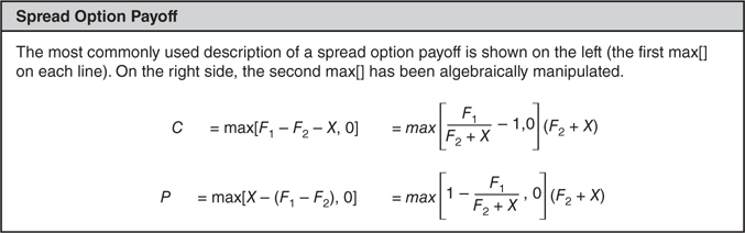
Figure 3.6.7 Spread option payoff
Modifying the formula to work as a ratio allows this payoff to be shoe-horned into a Black Scholes framework. Looking at the valuation formula, the primary difference between the Kirk’s approximation formula and the standard Black 76 formula is that the spread option gets multiplied by (F2 + X) and the F has changed from the distribution of future prices to the distribution of the ratio of F1 over F2 + X (Figure 3.6.8).
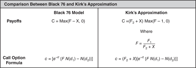
Figure 3.6.8 Comparison of Black 76 to Kirk’s approximation
The key complexity is determining the appropriate volatility that needs to be used in the equation. The “approximation” that defines Kirk’s approximation is the assumption that the ratio of two lognormal distributions is normally distributed. That assumption makes it possible to estimate the volatility needed for the modified Black Scholes–style equation (Figure 3.6.9). These formulas use the standard Black Scholes inputs (Figure 3.6.10). These formulas also use standard mathematical functions (Figure 3.6.11).

Figure 3.6.9 Spread option call formula
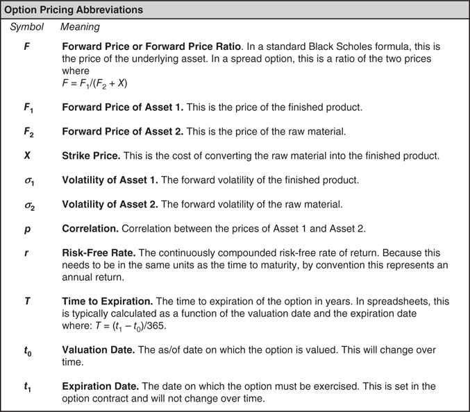
Figure 3.6.10 Option pricing abbreviations
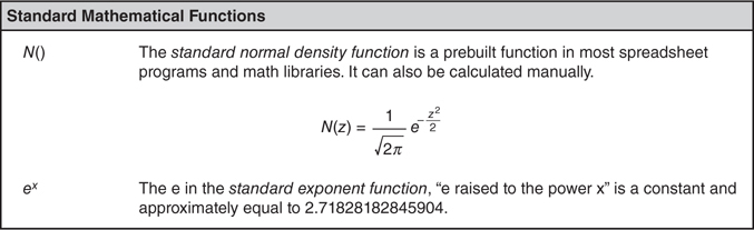
Figure 3.6.11 Standard mathematical functions
Estimating Implied Correlation
Unlike a more typical Black 76 formula, which has only one unknown parameter (implied volatility), a spread option will have three unknown parameters. It will have two implied volatility terms and an implied correlation term. While it’s easy to get sidetracked about what each of those values might mean under different contexts, in an option valuation the sole purpose of these parameters is to define the volatility of the ratio of the two assets in the future.
To understand what a ratio in the future might look like, both ratios and spreads can be historically observed—all it takes is historical pricing data. For example, examining a natural gas transportation spread, it is possible to look at the ratio of prices between natural gas prices at Florida Gas Pipeline Zone 3 (near Pensacola on the western part of the Florida Panhandle) and Florida City Gates (in central Florida near Orlando, Florida). It is possible to find the normal distribution that best fits historical observations using a spreadsheet (Figure 3.6.12).
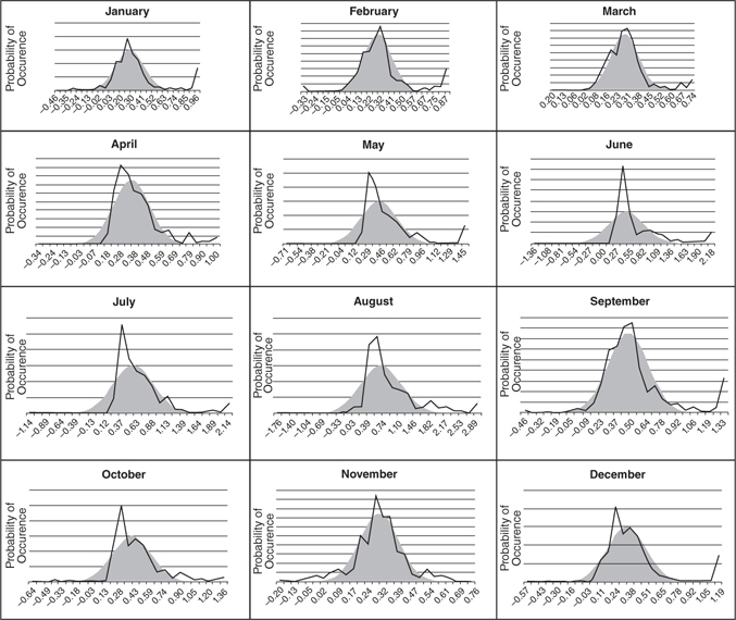
Figure 3.6.12 Historically observed spreads
Assuming that futures spreads look like historically observed spreads, it is possible to calculate the volatility of the normal distributions that best fit the historical data. Then, it is possible to find the Black Scholes implied volatility that defines that best fit distribution. Mathematically, this is relatively easy to calculate since a normal distribution is defined by a single variable, dispersion, and the dispersion in the random walk model used by Black Scholes scales in a predictable manner (with the square root of time).
This provides a way to examine correlation under normal conditions. One way to get around that problem is to use other markets to estimate two of the variables (like the asset volatilities) and solve for the remaining variable (the correlation) that results in the desired future distribution. Kirk’s approximation equation can be rearranged to solve for the implied correlation (Figure 3.6.13).
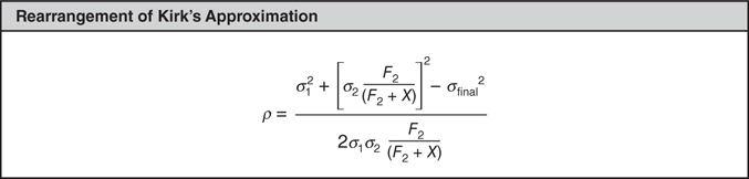
Figure 3.6.13 Kirk’s approximation, rearranged
Solving for the implied correlation this way, it is fairly common to observe negative correlations in the short term rise to a level above 90 percent after a couple of months.