4.2

THE GENERATION STACK

In deregulated areas, the coordinating Independent System Operator/Regional Transmission Operator (ISO/RTO) for the area holds daily auctions to determine the price of power. These are competitive auctions where power plants bid against one another for the right to produce power. The physical capabilities of each generator are a major factor in their bidding strategies. Consequently, the primary way to estimate power prices is to examine power providers ordered by their cost of production. This ordering is called a generation stack. For example, if there are four power plants on a power grid with 450 megawatts per hour (MWh) of total capacity, a generation stack ordered from highest cost (on top) to lowest cost (on the bottom) might look like Figure 4.2.1.

Figure 4.2.1 A generation stack

Dispatch capacity, often just called capacity, indicates how much power each power plant can produce. The break-even cost indicates the minimum price the power plant can accept for its power and still make a profit. For fuel-dependent power plants, like the natural-gas-fired generator, this cost will be heavily influenced by fuel costs.

This ordering can help predict the prices produced by the day-ahead and real-time auctions. In most cases, power plants will place bids above their own cost of generation (their break-even cost), and below the costs of the next type of unit in the stack (Figure 4.2.2). For example, the coal generator will probably place bids somewhere between $50 and $85. The price of power (on the left axis) can be predicted by looking at the predicted consumer demand (on the bottom axis).

Figure 4.2.2 Visual representation of a generation stack

The Mechanics of Day-Ahead and Real-Time Auctions

In most deregulated regions, there are two auctions that determine the clearing price of power. The first is a day-ahead auction; the second a real-time auction. The day-ahead auction uses predictions of the upcoming day’s load to schedule power plants the day before power is needed. This auction schedules power producers to be active for an entire hour. If the demand fluctuates throughout the hour, or if the load forecasts are incorrect, an adjustment will be needed to balance production with demand. Adjustments are made in the real-time auction.

In both auctions, generators [also called load serving entities (LSEs)] participate by submitting offer curves (their generation levels associated with prices they are willing to accept) and their technical constraints (startup costs, minimum up time, and so on). After collecting offers from generators, the ISO selects the winning generators that minimize the cost to the market. For example, a coal power plant with a cost basis of $50 might want 100 MWh of capacity always operating during the period. So, it places its first bid at $0 for its first 100 MWh. Then, it will start placing bids for greater amounts of power at progressively higher prices. The last bid is placed just under the $85 break-even cost of the next generation unit in the stack (Figure 4.2.3).

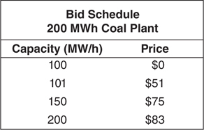
Figure 4.2.3 Bid schedule

When creating a bid, a generator needs to decide whether to attempt to sell all of its power in the day-ahead market or to reserve some capacity to sell into the real-time market. There are potentially greater profits in the real-time market, but the risk of being inactive is also higher. In both cases, bidding strategies are dictated by the physical characteristics of power plants. The most important characteristics are how quickly a power plant can come online and its efficiency at converting fuel into electricity. If a generator is not selected to operate in the day-ahead market, it is still eligible to participate in the real-time market.

Not every generator is capable of participating in the real-time market. The real-time auction requires that generators be capable of starting quickly and having their fuel supplies lined up. Inefficient power providers often have this capability. However, if a low-cost provider fails to sell their power in the day-ahead market, they often won’t be able to participate in the real-time market either. Most of the daily generation requirement is auctioned off in the day-ahead market—the real-time auction is used for balancing short-term fluctuations and unexpected demand.

Generation costs determine how most power providers participate in the daily auctions. Low cost providers want to lock in profits. They will have already lined up their fuel supplies and are probably hedging their price exposure in anticipation of being activated. If they don’t sell power in the day-ahead auction, they may be locked out of the real-time market by operating constraints. In comparison, higher price providers may benefit from waiting until the real-time auction if they can’t lock in sufficiently high prices early.

The Dispatch Stack

In deregulated markets, LSEs are placed into economic dispatch order based on the results of the day-ahead and real-time auctions held by each TSO. The lowest bidding LSEs are activated first, followed by higher bidders. The order that power plants are turned on is called the dispatch stack. This is a last on, first off ordering that is similar to a stack of plates (Figure 4.2.4). The unit at the top of the stack (the marginal unit) is the last unit to be activated and the first to be deactivated. The top of the stack is a very important location. The provider on the top of the dispatch stack sets the clearing price of power for a region. This provider is often called the marginal provider.

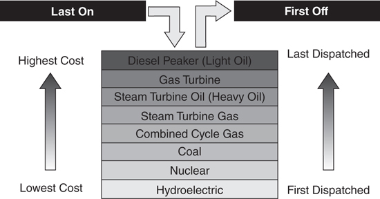
Figure 4.2.4 The dispatch stack

In most cases, the dispatch stack will be ordered similarly to the generation stack. The cheaper a power plant can generate power, the more it has to lose if it doesn’t get activated. Once the price of power rises substantially over a provider’s cost of production, the power provider will risk losing a large profit if it isn’t active. As a result, each power plant will usually actively bid only on a small portion of the generation stack—the part after it becomes profitable, but before it has too much money on the table. After that, they become price takers, allowing more aggressive bidders to set the clearing price of power.

Higher cost providers have a different problem—other power plants will know the break-even prices of the providers above them on the stack and bid just under that price. This behavior exists because everyone gets paid the same price for power—there isn’t an economic penalty for bidding just under a competitor if someone else sets a higher clearing price.

As a result, power plants with similar capabilities tend to cluster their bids around the same price points. Only a few power plants at any time actively set the price of power. Consequently, the couple of power plants on the margin have a disproportionate effect on the price of power. Because similar units cluster their bids, it is usually possible to determine a profile of the marginal producers.

Baseload, Mid-Merit, and Peaking Suppliers

It is common to describe each of the load providers within a generation stack as a baseload, mid-merit, or peaking unit. These terms broadly describe the behavior of power plants.

Baseload plants are located at the bottom of the generation stack. These power plants are active all year and sell power in the day-ahead auctions. They produce power cheaply, are expensive to shut down, and run continuously even when demand is at its lowest level. Hydro, nuclear, and coal plants all fall into this category. Hydro plants don’t have any fuel costs and may not be able to shut down without flooding nearby communities. Nuclear plants require the use of control rods to slow down their nuclear reactions. Without being cooled, a nuclear reaction will keep going at maximum capacity. It costs money to shut down a nuclear reactor. Coal plants are easier to shut down but can be expensive to restart if allowed to cool down completely. Coal plants are more costly than other baseload producers, but they have a huge cost advantage over other fossil fuel producers. Coal is by far the cheapest of the fossil fuels per Btu of energy. Almost all baseline plants run full time—they are rarely on the margin, and offer power at low costs in order to avoid going offline.

Peaking generation on the other extreme, provides short-term electricity during periods of peak demand (typically summer afternoons). These generators are at the very top of the generation stack. These plants need to start up quickly and be cheap to maintain. They don’t need to be cheap to operate—conserving fuel is an afterthought when power can be sold at sufficiently high prices. Many of these power plants are essentially jet engines. Fuel is pumped in and ignited; there are a minimum of moving parts and a lot of wasted heat energy. Many of these plants only operate a couple hundred hours a year. In order to recover costs, these plants will charge very high prices. These plants will operate almost exclusively in the real-time auction market except when day-ahead prices are extremely high.

Mid-merit plants are somewhere between the two extremes. In some cases, these plants are older, less-efficient baseload plants that are no longer cost effective enough to run full time. In other cases, these are highly efficient natural gas plants that are easier to cycle than the baseload generators. These generators are commonly on the margin, and show a lot of variability in their bidding strategies. Baseload generators are always going to bid low—they need to operate full time. Peaking generators are always going to bid high—they are extremely expensive to operate. Mid-merit generators are going to bid in both day-ahead and real-time markets, and will usually set the price of power.

Active Versus Passive Bidding Strategies

There is a fair amount of gamesmanship in choosing how to bid in power auctions. Generators want to get the highest possible price for their product. However, since there is a single price for power in a region, it isn’t important to be the top bidder. As long as a power plant is operating, it is getting the same price as the highest bidder. There is no downside to bidding a zero price if someone else sets the price at a higher level. In contrast, active bidding is risky—power plants that actively try to control the price of electricity run the risk of being inactive and not getting paid.

The basic decision on whether to actively participate in the bidding process, and risk being inactive, often comes down to how much money that a power plant stands to lose if it isn’t activated. A power plant’s profit is the spread between the price of power and the power plant’s cost of production. If a power plant has a very low cost of production, it will give up substantially more profit by being inactive than a plant with a higher cost of production.

For example, it might be possible for a power plant to increase the price of power by $1 if it is willing to bid aggressively into the day-ahead market. However, if aggressive bidders stand a 10 percent chance of being inactive, the decision is complicated for providers that are already highly profitable. If the price of power is around $100, it wouldn’t be worthwhile for a plant with a cost basis of zero to give up $10 (a 10 percent chance of being inactive and giving up $100) for a chance to make an extra $0.90 (making an extra dollar 90 percent of the time).

At the other extreme, a power plant with a very expensive cost of production would have a different reaction to the same decision. With a $95 cost of production, a power plant benefits substantially from aggressive bidding. In this case, the power plant would only give up $.50 (giving up a $5 profit, 10 percent of the time) for an extra $0.90 (an extra dollar 90 percent of the time).

Optimal Bidding Strategies

Most generators split their bid into several smaller bids. It is not uncommon for some of these bids to be offered at or below the generator’s cost of production. Since most generators are steam turbines that cost money to bring online, unaggressive bids ensure that the generator can avoid unnecessary stoppages. A power plant will often submit bids at higher prices in an attempt to maximize profits. Generally, the placement of the higher bids will depend on who else is bidding at that point.

For example, if a generator can profitably sell power at $50 and the next plant in the generation stack becomes profitable at $60, the first generator is likely to split their bid into two pieces—a piece below $50 to minimize the risk of being completely inactive, and the rest of their bid just under the $60 mark. Generally, this second bid will be as high as possible without tempting the next generator in the stack to undercut that price.

Bidding in this manner requires an in-depth knowledge of all the power plants around a certain point in the generation stack. In most cases, this is specialized knowledge learned through trial and error. Power generators usually have a detailed understanding of the generation stack around their own production costs. However, they won’t understand other parts of the stack with the same detail. As a result, most power plants only bid aggressively on the portion of the generation stack near their own costs of production.

Because of the need to prevent unnecessary shutdowns and restarts, most optimal bidding strategies do not simply react to prices. Optimal bidding incorporates predictions of likely future decisions into the current decision. In many cases, it is worthwhile for a steam turbine to take a loss in some periods to avoid startup costs in a later period. These simulations are often based on a Game Theory analysis.

Variable Generation

It is common for the generation stack to change throughout the day. In particular, many renewable power providers can’t supply a steady supply of power throughout the day. Solar power is a good example—it depends on sunlight. Sunlight is most abundant during the middle of the day. As a result, the generating capacity of a solar plant will be higher in the afternoon than in the early morning or late evening. The generation stack will change to account for this variable supply. Hydro power, wind generators, and imports and exports from other power grids are all examples of variable supplies of power.

In many cases, variable power providers can’t turn off their power supplies or guarantee delivery. For example, once power is scheduled to be imported from another power grid, it can’t be easily cancelled. Solar, wind, and hydro generators also can’t shut down on short notice. They also can’t guarantee that they will be able to deliver their power either. As a result, these power suppliers will be price takers—they will bid zero cost for their power and get paid the clearing price set by other market participants.

The production profile for a variable generator can change over time. Sometimes these changes are seasonally predictable, and other times they are random. It is usually possible to predict the variable supply of electricity a day ahead of time, but longer-term predictions become less accurate. For example, hydro power is very dependent upon seasonal rainfall that can occur anywhere within the space of a month or two. A day ahead of time, this water flow on the rivers will be well known. Likewise, solar power plants receive more sunlight in summer months but are also affected by cloudy conditions and precipitation. The most important impact is that even over small periods like a week or two, there can be substantial changes to variable production (Figure 4.2.5).

Figure 4.2.5 The variable generation in PJM on two different days in August 2005

Even small changes to the generation stack can have a major effect on prices because the top of the generation stack is getting displaced. During August 2005, power prices in PJM were around $80. A 4,000-megawatt (MWh) change in power might change the power prices by $10 or more as shown in Figure 4.2.6. The graph shows part of the PJM generation stack containing the marginal generators during August 2005 and the effect that an additional 4,000 MWh of power would have on prices.

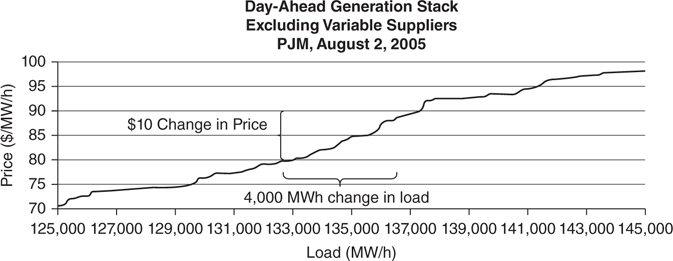
Figure 4.2.6 Small changes in supply can have a big impact on the price of power

Variable generation is a major reason why periods in the same day with identical consumer demand can see a wide range of prices. This makes it difficult to back into a generation stack by looking at daily loads and prices published by ISO/RTOs.

Estimating Break-Even Costs Using Heat Rates

No one, except for the ISO/RTO coordinating the daily auctions, knows the exact makeup of the generation stack until the data are released several years later. Auction bids are not made public, nor do load producers publish their break-even costs. To predict power prices, it is necessary to look at historical prices and estimate the generation stack from other pieces of information (Figure 4.2.7). For example, normalizing power prices by dividing them by fuel prices to create a heat rate graph is a common way to estimate changing power prices.

Figure 4.2.7 Generation stack

For fuel-dependent load providers, the cost of fuel and the conversion efficiency of their power plant combine to determine where they become cost effective. Natural gas prices are particularly important in determining the price of power because marginal producers commonly use that fuel. The natural gas/power relationship is so pervasive that it has its own terminology. The ratio of power prices to natural gas prices is called an implied market heat rate.

An implied market heat rate is easy to calculate—it is the average price of power divided by the average price of fuel in a specific geographic area. Because fuel needs to be paid for and scheduled for delivery ahead of time, the price of fuel within a particular day is constant. A generation stack can be described by either prices or heat rates as shown below. The heat rates are calculated by dividing the prices by $12.70 (the price of natural gas on that day).

When fuel prices rise, the break-even cost of power providers using that fuel will also rise. As a result, the generation stack for those producers will change. For example, in August 2005, the price of natural gas rose from $8.02 to $12.70. This coincided with a large move in the price of power (Figure 4.2.8). Power prices rose significantly for parts of the generation stack.

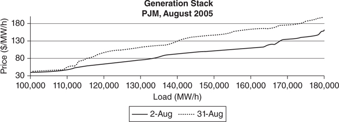
Figure 4.2.8 Generation stack shift

The implied market heat rate can identify how much of a change in electricity prices is due to a change in natural gas prices. If implied heat rates don’t change, the ratio between power and gas prices remains constant. A constant ratio means that the fuel prices fully account for the change in electricity prices. In August 2005, on the portion of the generation stack where natural gas plants are profitable, there was very little change in market heat rates between the two days (Figure 4.2.9). In Figure 4.2.9, the part of the generation stack where natural gas is the marginal fuel is highlighted.

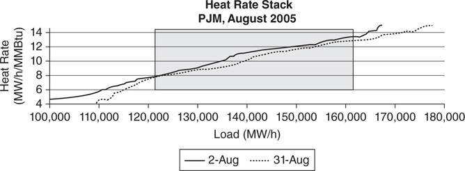
Figure 4.2.9 Heat rate stack

Day-Ahead and Real-Time Auctions

Although there are two separate auctions setting the price of power, the generation stack and the bidding strategies of power producers are nearly identical for both. Most of the generation capacity is locked in during the day-ahead market with a small amount of balancing required from the real-time market. Although there are fewer participants in the real-time auction, similar bidding dynamics lead to similar generation stacks. A comparison of real-time and day-ahead prices for two days can be seen in Figure 4.2.10. The auction prices are close together most of the time. Occasionally, prices in the real-time market are higher.

Figure 4.2.10 Day-ahead and real-time prices

The inability of many power plants to react quickly to changes in load is the reason for two auctions. Typically, the day-ahead market activates power plants in half-hour or hour-long increments. The load at the start of the period determines the number of power plants that get activated. However, if demand rises before another set of power plants is activated (either a half hour or hour later), that demand will need to be met by the real-time market (Figure 4.2.11). The relationship between changes in hourly demand and the short-term change in prices can be seen in Figure 4.2.11.

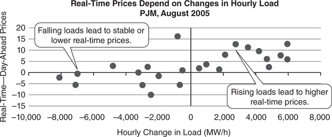
Figure 4.2.11 Changes in hourly loads

In most cases, marginal power suppliers tend to use the same strategy for participating in both auctions. The highly efficient generators at the bottom of the generation stack are the most likely to get locked out of the real-time market. However, except for periods of very low demand, the bottom of the generation stack will be continuously active, and won’t be on the margin. As a result, the real-time and day-ahead generation stacks are usually very similar.

Problems with Marginal Pricing

Marginal pricing works well for the certain generation stacks. For example, it worked well for the type of generation stack that existed in the mid-1990s—the type of stack that existed when power markets were first being created. These generation stacks were composed of cheap baseload coal or nuclear power. More expensive natural gas provided high marginal prices. Marginal pricing does not work as well when the generation stack is flat. By 2015, 20 years of new technology and an influx of cheaper natural gas that resulted from natural gas fracking had created a much flatter generation stack.

In power grids where all generators have similar marginal costs, the marginal pricing mechanism makes it difficult to make a profit. For example, if the marginal unit on a power grid is a 10 MMBtu/MWh heat rate unit, and gas prices are $10/MMBtu, then power prices would be approximately $100/MWh. If gas prices fall to $4/MMBtu, then marginal power prices fall to $40/MWh. For a baseload coal unit that might have a variable cost of $35/MWh, the profit drops from $65 dollars (the difference between $100/MWh and $35/MWh) to $5/MWh (the difference between $40/MWh and $35/MWh).

An extreme version of a flat generation stack will commonly occur when all market participants choose similar technology. In other words, when a power grid with only one technology uses marginal pricing, everyone’s marginal cost would be the same and no one would make a profit. Not making a profit is problematic because constructing new generation typically requires large initial investments that need to be recovered during operations. Anyone lending money to a developer will want to ensure that there is a steady stream of profits that can repay the cost of construction.