
9
GLOBALIZATION AND CLIMATE CHANGE: NEW EMPIRICAL PANEL DATA EVIDENCE
Maoliang Bu
Nanjing University School of Business & Hopkins-Nanjing Center
Chin-Te Lin
Université Paris 1 Panthéon Sorbonne Graduate School of Mathematics
Bing Zhang
State Key Laboratory of Pollution Control and Resource Reuse School of the Environment Nanjing University & School of Government Nanjing University
1. Introduction
In recent years, globalization and its effects on the environment have garnered enormous attention in connection with the heated debate over the so-called ‘pollution haven hypothesis (PHH)’, which argues that pollution-intensive industries will move from developed countries with stringent environmental regulations to developing countries with lax environmental regulations (Eskeland and Harrison, 2003; Copeland and Taylor, 2004; Bu et al., 2011; Cole et al., 2011). As a phenomenon, globalization has thus far proven to be too complicated to be examined through the lens of any single of its facets (such as its economic, cultural and political facets), thus indicating that a multi-angle spatial vision must be constructed (Held, 1999; Held and McGrew, 2003).
Previous studies of this subject in the economics literature have generally suffered from two main constraints. First, most studies rarely consider a sufficiently large number of countries, with most samples consisting of one or a few countries that do not provide a general global picture. Second, regarding the dimension of globalization, nearly all the studies take the form of either trade or foreign direct investment (FDI), and dimensions of globalization other than economic globalization have been largely ignored (Frankel, 2003).
FDI has been in the spotlight with regard to economic globalization because of the importance attributed to greenhouse gas (GHG) emissions and global warming. Held (1999) describes globalization as a historical process that transforms the spatial organization of social relations and transactions by developing transcontinental or interregional networks of interactions through which power is exercised. However, Albrow (1996) sees globalization in the spillovers of various actions, values, technology and products, which implies that – beyond economic globalization – the international political and organizational struggle and cross-cultural broadcasting are imperceptibly transforming our environment on a certain level through political and social globalization.
Pollution issues cannot be assessed from a single perspective. Since the mid-1980s, globalization has been associated with a remarkable growth in the level of popular concerns for political, economic and sociocultural issues – including pollution – on a global basis due to accelerated economic growth, intimate regional cooperation and widespread cultural broadcasting. Among the concerns, Rodrik and Wacziarg (2005) indicate that political institutions play a key role in global negotiations and have been recognized to exert an important influence on world economic growth. This recognition has attracted more attention to the link between political pluralism and economic liberalization and development, which may have led to increased pollution levels based on all the linkages. At approximately the same time, environmental reforms (mainly in OECD countries) also began to detach economic growth from intensifying environmental or ecological disruptions, which served to enable economic growth in some cases despite an absolute decline in resource consumption and pollution. In transition economies (mainly non-OECD countries), only an improving democracy has a significant effect on political and economic conditions (Rodrik and Wacziarg, 2005), which may lead to better environmental quality.
Generally, globalization not only eliminates border barriers around the world through its own pluralism but also liberalizes the circulation of investment and sociopolitical flows. However, while higher levels of globalization can mean the advancement of our society, it can also lead to environmental degradation. Because climate change is considered a challenge to our future development, an increasing amount of research has focused on untangling the relationship between the environment and how the multiple aspects of globalization affect different types of FDI and firms’ relocation choices – how technological and knowledge spillovers work in more than just an economic sense. However, it has thus far been difficult to understand the extent to which environmental quality is influenced by the current wave of social and political globalization.
Some research has intended to include political concerns – at least partially. For example, Barrett and Graddy (2000) find that increases in civil and political freedoms significantly improve environmental quality, and Fredriksson and Mani (2004) find that the combination of trade integration and political stability enhances the stringency of environmental regulation. Nonetheless, few researchers have explored globalization using a comprehensive analysis.
This paper aims to rectify this deficiency in the literature by integrating the theoretical principles developed by Grossman and Krueger (1991) with empirical panel data evidence and the new KOF globalization index. Adopting a panel data sample of 166 countries from 1990 to 2009, our results suggest that, on average, increased carbon emissions move in tandem with higher levels of economic, social and political globalization and that this effect varies by OECD and non-OECD country group. Further evidence reveals this coordinated relationship after we decompose the major contributors of carbon emissions to identify emissions from the manufacturing and construction sector. We therefore provides consistent evidence and further discussion of pollution haven effects in terms of climate change.
The remainder of this paper is organized as follows. Section 2 presents a literature review of pollution haven studies and the analysis framework. Section 5 presents our basic empirical strategy, including the model, the data and our instrumental variable (IV) method. Section 9 explains and discusses the estimation results. The conclusions are presented in Section 13.
2. Literature Review and Analytical Framework
2.1 Literature Review
Sanna-Randaccio (2012) summarizes the conclusions of several papers and indicates that the importance of low-carbon FDI from developed countries and emission-saving technology from multinational enterprises (MNEs) may improve the environmental quality in non-OECD countries by easing the degradation related to climate change. Thus far, empirical research (e.g., Frankel, 2009) based on cross-country data finds no support for pernicious effects of trade with certain measures of environmental degradation. In another summary of empirical studies, Erdogan (2014) indicates that empirical studies have not found widespread support for pollution haven effects that are triggered by FDI flows from developed to developing countries. The empirical evidence does suggest that trade and growth will lead to degradation of some environmental measures, but carbon emissions may be an exception. A number of pioneering papers by John List and a series of researchers have explored the time series properties of many types of pollutants to test the convergence of pollution levels across states and countries. Thus, Strazicich and List (2003) examine the convergence properties of carbon emissions over a panel dataset of 21 industrial countries from 1960 to 1997 and find evidence that carbon emissions patterns have converged. Brock and Taylor (2010) reinvestigate the Environmental Kuznets Curve (EKC) with a modified approach and connect the EKC to the Solow model. Using carbon emission data from 173 countries over the pre-Kyoto period, that is, 1960–1998, the evidence developed by Brock and Taylor (2010) also provides an answer for current disputes regarding the EKC and carbon emissions, as well as other pollutants. Some researchers believe that differences in carbon emissions evidence emerge because carbon emissions are an externality that can be addressed only at the global level (and not at the national level) because of free rider problems. Thus, institutions of governance are necessary at the multinational level, and these have not been in place until the recent wave of globalization.
As a result, globalization, economic growth and the environment may not necessarily be in conflict. Air pollution problems require both an adequate level of income and an effective mechanism of supervision and governance. Thus, externalities such as GHG emissions and other air pollutants are likely the consequence of global interactions. National governments cannot address these types of externalities on an individual basis but only with a global mechanism. Our research contributes mainly by attempting to provide a general overview to elucidate these problems and to show how globalization is linked to environmental problems and the heated debates involving carbon emissions.
2.2 Analysis Framework
The pioneering work by Grossman and Krueger (1991) is central to this paper. It not only led to a subsequent burgeoning literature on the EKC but also developed a convention of decomposing trade's influence on the environment into three categories of effects: technological, scale and compositional. These three categories are assumed to have positive, negative and unknown effects on the environment, respectively. Within this framework, beyond economic globalization, we integrate other dimensions of globalization, including social globalization and political globalization as we move toward an analysis of globalization's effects on the environment. The theoretical predictions of the effects of globalization on the environment are summarized in Table 1. First, with economic globalization, the effects are straightforward and are similar to those addressed in Grossman and Krueger (1991). Second, social globalization, as defined in the KOF index, indicates increasing linkages among international news, books, McDonalds, and the Internet. It is a process through which more international social integration might generate more environmental technology spillovers that lead to better environmental quality. Meanwhile, this process also brings changes in lifestyle and consumption from developed to developing countries that are not necessarily environment or carbon friendly. Third, political globalization, which is often ignored by economists, directly impacts how international institutions work and bring about change (e.g., the international conferences on climate change).
Table 1. Theoretically Predicted Effects of Globalization on the Environment.
| Economic | Social | Political | |
| globalization | globalization | globalization | |
| Technology effect | + | + | ? |
| Scale effect | – | ? | ? |
| Composition effect | +/– | ? | ? |
| Overall | ? | ? | ? |
Note: +/–/? stand for positive/negative/unknown effect, respectively. The table integrates the author's work with Grossman and Krueger (1991).
Given that the mechanisms for why and how social and political globalization affect carbon emissions are less straightforward than those for economic globalization, further explanations based on previous studies must be explored. With regard to social globalization, there are at least three alternative but non-exclusive theoretical explanations, namely, transportation, lifestyle changes and technology spillovers. First, as critical drivers of globalization, transport systems (as one important component of social globalization) have contributed greatly to carbon emissions. Taking the example of air transport, between 1990 and 2004, GHG emissions from aviation increased by 86%. In the case of India, between 2005 and 2007, domestic airline companies ordered a total of 500 new airplanes from aircraft manufacturers Airbus and Boeing to cover new travel needs. Second, given limited natural resources, environmentalists have long warned developing and transition countries about trying to emulate Western lifestyles. However, due to the wave of social globalization, the South has actually been catching up to the North in terms of lifestyle, even though the income gap between the South and the North has not significantly decreased. These lifestyle changes are often associated with deforestation, which makes carbon emissions even worse. Third, unlike the previous two mechanisms, social globalization can also be positively related to reductions in carbon emissions, such as through technology spillovers. That is, more personal contacts and information flows stimulate more spillovers of environmental friendly technologies. In addition, such changes also bring more environmental awareness to developing countries. For example, since Beijing Olympic Games (a good example of social globalization), the Chinese authorities introduced a partial ban on car traffic in the city.
With regard to the mechanisms for political globalization's effects on carbon emissions, political scientists have gradually included climate politics in mainstream political science research (Bernauer, 2013). Spilker (2012a, 2012b) suggests three mechanisms for how membership in intergovernmental organizations (IGOs) impacts the environmental performance of developing countries. First, at least in principle, IGOs can compel member states to obey their rules by raising the reputational stakes for reneging on agreements. Second, IGOs create norms that define good behaviour – and what constitutes bad conduct. Third, although countries become members of an IGO for specific reasons, for example, financial assistance, they are also exposed to the other purposes of the organization, such as environmental protection. For example, by joining the Association of Southeast Asian Nations (ASEAN) in 1997, Laos was required to implement a number of agreements pertaining to making agri-economic development more sustainable, which as a side effect positively affected Laos's environment. When applying the above three mechanisms to the specific issue of carbon emissions, however, we must remember the differences between developed and developing countries. Taking the Kyoto Protocol as an example, the Annex I Parties with carbon reduction targets are generally developed countries, while developing countries generally do not have carbon reduction targets. Given this difference, it is not diffucult to understand the recent report by the International Energy Agency (IEA) stating that the carbon dioxide (CO2) emissions of developing countries “increased at a much faster rate” than the CO2 emissions of industrialized countries.
To summarize, the influence of social and political globalization on climate change deserves at least equal attention as economic globalization. To some extent, economic integration can actually be regarded as the result of political arrangements and social/cultural proximity. Balli and Pierucci (2015) highlight the role of political and social globalization in the following question: if political and social globalizations are taken into account, does economic integration still play a role? Although our paper investigates the three aspects of globalization separately, it will be interesting to compare the extent of each. We will return to this point later when we discuss the empirical results.
Therefore, using the globalization index (KOF), we hope to present a fresh perspectives on how developed and developing countries compete and interact with one another under the framework of globalization. We intend to discuss the heated debates on pollution havens in combination with the multi-faceted aspects of globalization and other hypotheses addressed by economists, sociologists and political scientists.
3. Empirical Strategy
3.1 Model
Following Grossman and Krueger (1991), we begin by estimating the following reduced-form equation for the time variation with countries to identify the effects of globalization on the environment. We predict outwards to see whether income will converge by controlling income per capita and its square term. The panel data model is a time-variant model that explains pollutant emissions in country i and period t by:
where Epc is per capita pollutant emissions denoting the pollutant emission variable, γ represents country-specific intercepts, θ represents time-specific intercepts, and economic structure represents the manufacturing value added to the GDP to capture the structural change over time and Y represents per capita GDP in logarithms of constant year US $. The square term of Y is also included in the model following the classic setting of the Environmental Kuznets Curve which is an inverted U shape. The scatterplot for carbon emissions and GDP per capita is presented in Figure 1, which intuitively supports the inverted U shape instead of a N or S shape.1
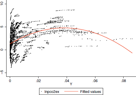
Figure 1. Carbon Emissions and GDP per Capita.
Note: The figure shows the relationship between carbon emissions and GDP per capita with full sample. The left axis indicates the emissions level of CO2 in logarithm.
Gindex refers to the level of globalization using the KOF index, which is based on 23 variables that relate to the different dimensions of overall globalization in 207 countries (we consider the overall globalization index for 161 countries, the economic globalization sub-index for 135 countries, the social globalization sub-index for 163 countries and the political globalization sub-index for 166 countries). The overall index and the sub-indices assume values scaled from 1 (minimum globalization) to 100 (maximum globalization). The 2015 KOF globalization index is available for the 1970–2011 period. These 23 variables are consolidated into six groups, and the groups are further combined into three sub-indices and one overall index of globalization in reasonable percentages derived using an objective statistical method (Dreher 2006; Dreher and Gaston, 2008; Dreher et al., 2008b). In this research, we adopt the 1990–2009 data to examine globalization's effect on pollutant emissions. The three sub-indices of globalization lead us to the following equation:
where Sub-index refers to the level of economic globalization, social globalization or political globalization, respectively and separately.
According to the KOF index, these types of globalization are defined as follows:
- Economic globalization is characterized as two main group variables: (i) actual flows (trade, foreign direct investment, portfolio investment, and income payment to foreign nationals) and (ii) restrictions (hidden import barriers, mean tariff rate taxes on international trade, and capital restrictions).
- Social globalization includes three groups of variables: (i) data on personal contacts (telephone traffic, transfers, international tourism, foreign population, international letters), (ii) data on information flows (internet users, television, trade in newspapers) and (iii) data on cultural proximity (number of McDonald's restaurants, number of IKEA stores, trade in books).
- Political globalization is characterized by four different variables: embassies in foreign countries, national membership in international organizations, participation in U.N. Security Council Missions, and international treaties.
3.2 Data Resource and Descriptive Statistics
The data source for Epc is from Climate Data Explorer (World Resources Institute, 2015), which provides comprehensive data on greenhouse gas emissions.2 Given the accessibility of data we adopt three different measurements for the dependent variable (Epc): overall GHGs, overall CO2 and CO2 from the manufacturing and construction sector. The relationship between these three measures can be described as follow. According to the database, CO2 emissions is the major component of overall GHG emissions, which consists of four different types of emissions, with total CO2 at 73% on the average and the rest at 27% (overall totals of CH4, N2O and F-gas). Moreover, as for CO2 emissions itself, three sectors produce the majority, of emissions, namely, transportation (22%), electricity and heat (42%), manufacturing and construction (19%). Because the manufacturing and construction sector is more associated with the pollution haven effect, we therefore focus on this sector to test the effect.
Table 2 reports the data sources and the descriptive statistics for two country subgroups. We use two country subgroups for the 1990–2009 period (see the Appendix Table A1 for countries includ in this research) for two reasons: first, this research tries to examine how long the period of globalization after the 1980s affected the environment; second, previous research mainly addressed the carbon emissions problem in the pre-Kyoto period (before 1998). Frankel (2009) suggests that since the common view of a series of international environmental protocols settled down, we might observe the influence among all countries by considering an extended time period after 2000. In Figure 2, we show the relationship between GHG emissions and the overall globalization index in a subsample. In most cases, our findings indicate that comparatively lower globalization levels with higher pollutant emissions characterize the majority of non-OECD countries, with a correlation coefficient of 0.41.
Table 2. Variable Definitions and Descriptive Statistics.
| OECD countries (n = 24) |
Non-OECD countries (n = 142) |
||||||||||
| Variable | Definitions & source | Mean | Std. Dev. | Min | Max | Obs. | Std. Dev. | Min | Max | Obs. | |
| Overall globalization (1990–2009) | Dreher (2006) and Dreher et al. (2008b) | 75.32 | 14.78 | 29.67 | 92.50 | 480 | 15.21 | 11.47 | 92.38 | 2948 | |
| Economic globalization (1990–2009) | Dreher (2006) and Dreher et al. (2008b) | 72.96 | 14.19 | 19.59 | 95.62 | 460 | 17.43 | 9.94 | 99.16 | 2413 | |
| Social globalization (1990–2009) | Dreher (2006) and Dreher et al. (2008b) | 71.79 | 19.07 | 8.38 | 93.68 | 480 | 19.29 | 6.95 | 93.16 | 2988 | |
| Political globalization (1990–2009) | Dreher (2006) and Dreher et al. (2008b) | 85.79 | 13.52 | 14.19 | 98.26 | 480 | 22.34 | 1 | 98.43 | 3048 | |
| Ln(GDP per capita) | (Million constant (2005) US$), | 10.37 | 0.48 | 8.51 | 11.36 | 480 | 1.34 | 3.91 | 10.96 | 2952 | |
| WDI 2015 | |||||||||||
| Ln(GDP square per capita) | (Million constant (2005) US$), | 107.79 | 9.65 | 72.42 | 129.13 | 480 | 20.71 | 15.30 | 120.326 | 2952 | |
| WDI 2015 | |||||||||||
| Ln(Greenhouse gas) | MtCo2e, CIAT | 5.16 | 1.58 | 1.01 | 8.83 | 460 | 2.12 | –3.33 | 9.13 | 3027 | |
| Ln(CO2 emission) | MtCo2, CIAT | 4.83 | 1.63 | 0.64 | 8.67 | 480 | 2.42 | –3.81 | 8.93 | 3075 | |
| Ln(Manufacturing & construction) | MtCo2, CIAT | 3.09 | 1.57 | –0.77 | 6.55 | 480 | 2.10 | –4.61 | 7.71 | 2095 | |
| Economic structure | Manufacturing, value added (% of GDP) | 17.28 | 4.45 | 5.25 | 30.23 | 442 | 7.81 | 0 | 43.54 | 2559 | |
| WDI 2015 | |||||||||||
| Predicted trade openness (1990–2008) | Eppinger and Potrafke (2016) based on data by Felbermayr and Gröschl (2013) | 47.76 | 25.39 | 10.72 | 144.06 | 449 | 42.72 | 1.39 | 541.12 | 2555 | |
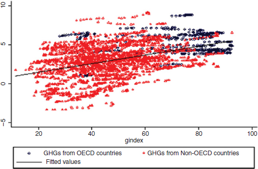
Figure 2. GHG Emissions and Overall Globalization in the Cross-Section.
Note: The figure shows GHG emissions (from 1990 to 2009) and overall globalization index (from 1990 to 2009) by country type. The left axis indicates the emissions level of GHGs in logs. The correlation coefficient is 0.43.
3.3 Instrumental Variable Method
Since the globalization index may be endogenous in the FE estimation, the instrumental variable method is adopted to tackle this issue. Following Felbermayr and Gröschl (2013) and Eppinger and Potrafke (2016), we use the exogenous component of trade openness predicted by geography and natural disasters as an IV for globalization variables in our model.
Frankel and Rose (2005) have attempted to isolate the effects that trade has independent of income by means of a gravity model3 by first considering the relationship between pollution and income. They find consistent support for the EKC in much of the literature for all three air pollution types (SO2, NOx and PM). However, the results regarding CO2 emissions are not consistent with our findings. Felbermayr and Gröschl (2013) show that natural disasters in one country influence the trade of its trading partners and develop a concept that is best illustrated with the following example: An earthquake affecting country A will increase the trade volumes of other countries to country A. Moreover, the trade increases will be larger when a trading country is located closer to country A. Eppinger and Potrafke (2016) elaborate upon this notion and address the causality problems by proposing that the geographic component of trade openness from the original model proposed by Frankel and Romer (1999) should be an IV for globalization. Felbermayr and Gröschl (2013) further suggest the importance of considering the exogenous component of geography and natural disasters in predicting trade openness as an IV for globalization. Therefore, the difference between Frankel and Romer (1999) and Eppinger and Potrafke (2016) is that their identification strategy is designed explicitly for the income-growth-nexus but not for examining the influence of globalization. Therefore, Frankel and Romer's (1999) results are not robust to the inclusion of geographic controls in the second stage of the model. Eppinger and Potrafke (2016) mainly address this problem by controlling for any observed or unobserved country-specific effects in their panel approaches which allows the use of IVs in a panel data model and for the control of the bias.
Eppinger and Potrafke (2016) build their IV model by improving upon the Frankel and Romer (1999) model and their IV is generally constructed in two steps: Eppinger and Potrafke (2016) estimate a reduced gravity model on a large sample of country pairs that explains the bilateral trade openness of country i to trade with country j in year t by natural disasters in country j. They further apply Poisson Pseudo Maximum Likelihood (PPML) to predict their instrumental variables. The modified gravity equation proposed by Frankel and Romer (1999) is grounded in their methodology, which explains the bilateral trade openness (the sum of imports and exports as a share of GDP) of the trade between country i and country j in year t with respect to country j following natural disasters in country j and the disaster variables that are exogenous to country i are shown as
From Equation (3), Eppinger and Potrafke (2016) generally obtain a predicted value for yearly bilateral trade openness – the IV adopted in this paper. The identifying assumption in the model of this research is that natural disasters in third countries have no effect on the pollutant emissions of a country other than through trade. In any event, similar omitted variables that influence growth, such as geographic and cultural characteristics, would also bias the estimates of trade openness. As a variable in the second stage, the model includes a large sample of country pairs that explains bilateral trade openness (the sum of imports and exports as a share of GDP) of country i to trade with country j in year t following natural disasters in country j, population, bilateral geographic variables (the logarithm of bilateral distance and a border dummy), and several interactions of the disaster variable. Following Frankel and Romer (1999), the model also includes a border dummy (equal to one for neighbouring countries) and the interaction terms assume that disasters in large countries, neighbouring countries, and countries that are closer to financial centres have stronger effects on bilateral openness measures. To best determine the effectiveness of the IV, we include our first stage regression results in all of our estimation result tables in the following form, where ∂FGit − 1 denotes the one-year lag in predicted trade openness as suggested by Eppinger and Potrafke (2016)4.
4. Empirical Results
4.1 Results using the Overall Globalization Index
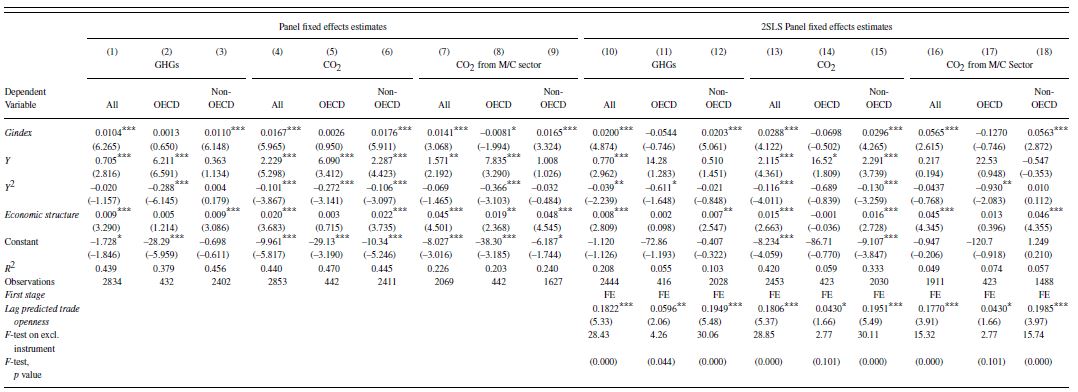
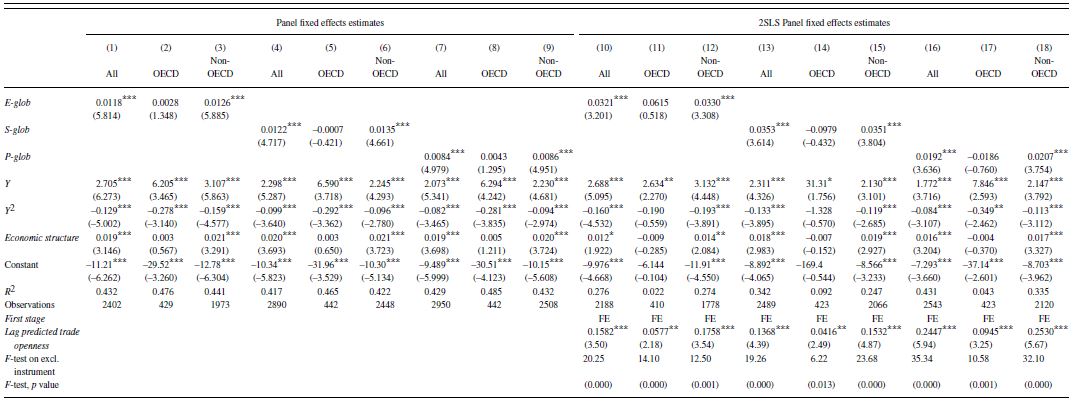
We start by reporting the results using the overall globalization index; we report the results using the sub-globalization index in later sub-sections. Table 3 presents the results for all three dependent variables (GHG, CO2 and CO2 from the manufacturing and construction sector). For every three columns in Table 3 (also in Tables 4–6), the first is based on the full sample and, the second and third are based on the OECD and non-OECD subsamples, respectively, in order to ease comparisons among them. Columns 1–9 of Table 3 show the initial results using the overall globalization index with the fixed effect estimation, and the 2SLS estimation results follow in columns 10–18. The results are robust to standard errors corrected for heteroskedasticity and are clustered at the country level. As shown in Table 3 columns 1, 4 and 7, the coefficient of the overall globalization index is positive and reaches the 1% significant level. This result suggests that an increased globalization level is associated with higher environmental pollution. We further compare the differences in the results for OECD and non-OECD countries. The initial results support the pollution haven effect for different performances with increased globalization in terms of climate change. The only negative and significant result in column 8 at the 10% level suggests a necessary discussion on carbon emissions from the industrial subsector, although the inference is not necessary true for OECD countries.
Table 3. Regression Results with Overall Globalization Index (All Pollutants).
Note: Asterisks indicate significance levels: *p < 0.1, **p < 0.05, ***p < 0.01.
Robust t-statistics for FE estimates and z-statistic for 2SLS estimates reported in parenthesis (standard errors clustered by country). Instrumental Variable: Lag predicted trade openness (Felbermayr and Gröschl, 2013) and (Eppinger and Potrafde, 2016).
Table 4. Regression Results with Globalization Index (Overall Green House Gas Emission).

Note: Asterisks indicate significance levels: *p < 0.1, **p < 0.05, ***p < 0.01.
Robust t-statistics for FE estimates and z-statistic for 2SLS estimates reported in parenthesis (standard errors clustered by country).
Instrumental Variable: Lag predicted trade openness (Felbermayr and Gröschl, 2013) and (Eppinger and Potrafde, 2016).
Table 5. Regression Results with Globalization Index (Overall Carbon Emission).
Note: Asterisks indicate significance levels: *p < 0.1, **p < 0.05, ***p < 0.01.
Robust t-statistics for FE estimates and z-statistic for 2SLS estimates reported in parenthesis (standard errors clustered by country).
Instrumental Variable: Lag predicted trade openness (Felbermayr and Gröschl, 2013) and (Eppinger and Potrafde, 2016).
Table 6. Regression Results with Globalization Index (Carbon Emissions from Manufacturing and Construction Sector).

Note: Asterisks indicate significance levels: *p < 0.1, **p < 0.05, ***p < 0.01.
Robust t-statistics for FE estimates and z-statistic for 2SLS estimates reported in parenthesis (standard errors clustered by country).
Instrumental Variable: Lag predicted trade openness (Felbermayr and Gröschl, 2013) and (Eppinger and Potrafde, 2016).
Our results also suggest that the higher the proportion of GDP derived from manufacturing is, the worse the environmental quality will be. In addition, the results are clearer for OECD countries, which we can attribute to the advantages of cleaner technologies, cleaner production procedures and effective environmental regulations in improving environmental quality, even with a higher contribution to GDP from manufacturing. Otherwise, this finding may be consistent with the pollution haven hypothesis, such that developed countries move their heavy polluting industries to non-OECD countries.
The 2SLS estimation results are presented on the right side of Table 3 (columns 10–18), which take the one-period lag of the predicted trade openness as an instrumental variable following Eppinger and Potrafke (2016). In the first stage, the IV has a significant effect on globalization across our panel with an F-statistic above Stock and Yogo's (2005) 20% critical value. These findings suggest that the partial correlation described in the OLS model slightly rejects a causal effect of globalization on pollutant emissions. We report 2SLS estimates based on the full panel set for the period from 1990–2009, although the entire one-year lag predicted trade share might not have a strong effect on the KOF globalization index in full periods of our data, indicating a potential problem of a weak IV. In general, the results of 2SLS estimations in Table 3 consistently support by the prior results. Further detailed discussion, including sub-indicator effects of globalization on pollution, is provided in the following section.
4.2 Greenhouse Gas and Carbon Emissions
After investigating the effect of overall globalization on climate change, we now decompose the overall globalization index into three sub-indexes and report the individual effects of each. Tables 4 and 5 present the results using as dependent variable of GHGs and CO2 respectively, considering the separate effects of three sub-globalization indexes economic, social and political.
As discussed earlier, we are more interested in the comparisons between different country groups. As shown in columns 2, 5 and 8 for the OECD countries and columns 3, 6 and 9 for the non-OECD countries in both Tables 4 and 5, the coefficient of the economic, social and political index is still positive and significant in columns 3, 6 and 9. However, it is not significant in columns 2 and 5 and 8 in both Tables 4 and 5. Therefore, it can be inferred that an increased level of economic, social and political globalization is associated with higher pollutant emissions for non-OECD countries. In addition, the results for the sub-globalization index for GHGs and carbon emissions show that increased globalization – whether economic, social or political globalization – leads to higher environmental degradation for non-OECD countries. However, a significant effect cannot be found for OECD countries. Based on these results, we cannot prove that the significant increase in the volume of emissions in non-OECD countries is associated with the transfer of pollution from OECD countries. Conversely, MNEs may demonstrate some positive effects from technology spillovers through a variety of globalization channels or greener FDI. Therefore, increasing emissions in non-OECD countries may be regarded as a reflection of long-run progress and economic transition. Thus far, this initial finding for greenhouse gas and carbon emissions might not sufficiently clarify the debate regarding whether a higher level of globalization will result in the transfer of polluters from home countries to developing countries using aggregate indicators. Therefore, we take one step further to analyse the major concern of pollution haven effects – carbon emissions from the manufacturing and construction sector.
4.3 CO2 emissions from the Manufacturing and Construction Sector
The results for carbon emissions from the manufacturing and construction sectors are reported in Table 6. In Section 10, we reported that overall globalization has a negative coefficient at a 10% significant level in column 8 (OECD country) of Table 3. This finding indicates that increased globalization positively affects the contribution of the manufacturing and construction sector in improving the environmental quality in OECD countries. However, the mechanism under globalization is not clear from these initial results. Our evidence from the estimation of the sub-dimensions of globalization in Table 6 further supports the pollution haven effects, demonstrating that higher economic, social and political globalization leads to a cleaner environment in OECD countries and to almost continuous environmental degradation in non-OECD countries.
The evidence from the manufacturing and construction sector directly supports the existence of pollution haven effects between OECD and non-OECD countries. There are two main causes for these pollution haven effects in the manufacturing and construction sector. First, theoretical research (Sanna-Randaccio and Sestini, 2012) suggests that the fear of moving all production abroad by means of FDI between two countries (with and without more stringent climate measures) is mainly due to high transport costs. However, Reinaud (2008) analyses job losses in the home country and direct carbon emissions increases in less environmentally stringent countries and finds that characteristics such as low income, high labour intensity, and comparatively lower environmental standards characterize non-OECD countries but that the actual transfers from the polluting manufacturing and construction industries occur not only by means of FDI but also through regional integration and cultural unifications.
Second, it is not only economic globalization that enables OECD countries to shift those high-carbon industries to developing countries, but also political and social globalization. More interestingly, our findings support the view of Balli and Pierucci (2015) who argue that the role of political and social globalization can be even larger than that of economic globalization. Indeed, in columns of 2, 5 and 8 of Table 6, the absolute value of the coefficient of political globalization (0.0069) and social globalization (0.0072) are greater than that of economic globalization (0.0020). This finding again highlights that globalization should not be simplified to only economic globalization.
Potential endogeneity problems associated with globalization may bias the estimation results. In general, the results of the IV models (as shown on the right side of Table 6) are consistent with the results of the previous FE models. The coefficient of economic social and political globalization on emissions from the manufacturing and construction subsector in the OECD country sub-sample were not significant. In the first stage, the IV has a positive and significant effect on globalization and the three sub-globalization indicators with an F-statistic above the Stock and Yogo's (2005) 15% critical value. We further do the Hausman test for the comparison between the favour of FE and 2SLS models. The test results generally favor the FE models, regarding the inference of non-OECD counties remains unchanged.
5. Conclusion
This paper investigates the relationship between globalization and climate change by adopting the new KOF globalization index and carbon emissions data. Our results suggest that, on average, increased carbon emissions move in tandem with higher levels of economic, social and political globalization and this effect varies by OECD and non-OECD country group. Further evidence adopting data from the manufacturing and construction sector suggest that globalization is negatively related to emissions from OECD countries but positively related to emissions from non-OECD country group. These findings jointly support the pollution haven effects in terms of climate change. Our estimation results are robust to different model settings, alternative dependent variable measurements and the adoption of IV methods.
To the best of our knowledge, this analysis is the first that links climate change and globalization in a broad sense (previous studies mainly focus on either trade or FDI) based on large scale sample data. We believe that such analysis can shed some light on the field on globalization and the environment, and contribute to the global policy making on climate change issues.
Acknowledgements
The authors thank two anonymous referees and editor Siqi Zheng for very helpful comments. They are also thankful for valuable comments from Donald A. R. George, Kenichi Imai, Chi-ang Lin, Leslie Oxley and other participants at the Journal of Economic Surveys 2016 Special Issue and International Conference: The Economics of Climate Change in August 2015 in Taipei, Taiwan. The first author is grateful for the support of the Alexander von Humboldt Foundation. This paper is supported by the National Science Foundation of China (Grant No. 71273004, 71322303 & 71403117), the Science Foundation of Jiangsu Province (No. BK20130572) and the fund from China's Ministry of Education (No. 14JHQ017).
Notes
References
- Albrow, M. (1996) Global Age. Oxford: Blackwell Publishing Ltd.
- Balli, F. and Pierucci, E. (2015) Globalization and international risk-sharing: do political and social factors matter more than economic integration? No.2015-04. Centre for Applied Macroeconomic Analysis, Crawford School of Public Policy, The Australian National University.
- Barrett, S. and Graddy, K. (2000) Freedom, growth, and the environment. Environment and Development Economics 5: 433–456.
- Bernauer, T. (2013) Climate change politics. Annual Review of Political Science 16: 421–448.
- Brock, W.A. and Taylor, M.S. (2010) The green Solow model. Journal of Economic Growth 15: 127–153.
- Bu, M., Liu, Z. and Gao, Y. (2011) Influence of international openness on corporate environmental performance in China. China & World Economy 19: 77–92.
- Cole, M.A., Elliott, R.J.R. and Okubo, T. (2011) Environmental outsourcing. Discussion Paper Series DP2011-12. Research Institute for Economics & Business Administration, Kobe University.
- Copeland, B.R. and Taylor, S. (2004) Trade, growth, and the environment. Journal of Economic Literature 42: 7–71.
- Dreher, A. (2006) Does globalization affect growth? Evidence from a new index of globalization. Applied Economics 38: 1091–1110.
- Dreher, A. and Gaston, N. (2008) Has globalization increased inequality? Review of International Economics 16: 516–536.
- Dreher, A., Gaston, N. and Martens, P. (2008b) Measuring Globalisation – Gauging Its Consequences. New York: Springer.
- Eppinger, P. and Potrafke, N. (2016) Did globalization influence credit market deregulation? The World Economy 39(3): 426–443.
- Erdogan, A.M. (2014) Foreign direct investment and environmental regulations: a survey. Journal of Economic Surveys 28: 943–955.
- Eskeland, G.S. and Harrison, A.E. (2003) Moving to greener pastures? Multinationals and the pollution haven hypothesis. Journal of Development Economics 70: 1–23.
- Felbermayr, G. and Gröschl, J. (2013) Natural disasters and the effect of trade on income: a new panel IV approach. European Economic Review 58: 18–30.
- Frankel, J.A. and Romer, D. (1999) Does trade cause growth? American Economic Review 89: 379–399.
- Frankel, J.A. (2003) The environment and globalization. Working Paper No. 10090. Cambridge, MA: National Bureau of Economic Research.
- Frankel, J.A. and Rose, A.K. (2005) Is trade good or bad for the environment? Sorting out the causality. Review of Economics and Statistics 87: 85–91.
- Frankel, J.A. (2009) Environmental effects of international trade. Harvard Kennedy School Faculty Research Working Paper RWP 09-006.
- Fredriksson, P.G. and Mani, M. (2004) Trade integration and political turbulence: environmental policy consequences. Advances in Economic Analysis & Policy 4(2), Article 3.
- Grossman, G.M. and Krueger, A.B. (1991) Environmental impacts of a North American Free Trade Agreement. Working Paper No. 3914. Cambridge, MA: National Bureau of Economic Research.
- Held, D. (1999) Global Transformations: Politics, Economics and Culture. Stanford, CA: Stanford University Press.
- Held, D. and McGrew, A. (2003) Political globalization: trends and choices. In I. Kaul, P. Conceicao, K. Le Gouven, and R.U. Mendoza (eds.), Providing Global Public Goods: Managing Globalization (pp. 185–224). Oxford: Oxford University Press.
- Reinaud, J. (2008) Issues Behind Competitiveness and Carbon Leakage. Focus on Heavy Industry. IEA Information Paper 2. Paris: IEA.
- Rodrik, D. and Wacziarg, R. (2005) Do democratic transitions produce bad economic outcomes? American Economic Review 95: 50–55.
- Sanna-Randaccio, F. (2012) Foreign Direct Investment, Multinational Entreprises and Climate Change. Milan: Fondazione Eni Enrico Mattei (FEEM).
- Sanna-Randaccio, F. and Sestini, R. (2012) The impact of unilateral climate policy with endogenous plant location and market size asymmetry. Review of International Economics 20: 580–599.
- Spilker, G. (2012a) Helpful organizations: membership in inter-governmental organizations and environmental quality in developing countries. British Journal of Political Science 42(02): 345–370.
- Spilker, G. (2012b) Globalization, Political Institutions and the Environment in Developing Countries. New York and London: Routledge
- Stock, J. H. and Yogo, M. (2005) Testing for weak instruments in linear IV regression. Chapter 5 in Identification and Inference in Econometric Models: Essays in Honor of Thomas J. Rothenberg, edited by DWK Andrews and JH Stock.
- Strazicich, M.C. and List, J.A. (2003) Are CO2 emission levels converging among industrial countries? Environmental and Resource Economics 24: 263–271.
- World Resources Institute. (2015) CAIT Climate Data Explorer. Washington, DC: World Resources Institute. Available at: http://cait.wri.org (accessed on March 5, 2015)
Appendix
Table A1. List of Countries Considered in this Research

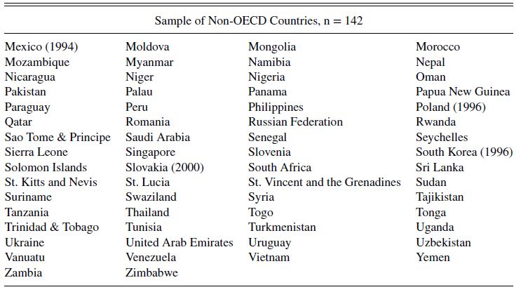
Note: Many countries participate in OECD after 1961 (the beginning of OECD). Therefore, following the previous empirical researches’ design on sub-sample regression, once a country participates in OECD group after 1990, we will regard that country as non-OECD country across our time period from 1990 to 2009. The join time of those non-original members are reported in parenthesis.