
4
THE DECOMPOSITION AND DYNAMICS OF INDUSTRIAL CARBON DIOXIDE EMISSIONS FOR 287 CHINESE CITIES IN 1998–2009
Maximilian Auffhammer
UC Berkeley & National Bureau of Economic Research
Weizeng Sun
Jinan University & Tsinghua University
Jianfeng Wu
Fudan University
Siqi Zheng
Department of Urban Studies and Planning, Massachusetts Institute of Technology & Hang Lung Center for Real Estate, Tsinghua University
1. Introduction
Urban energy use significantly contributes to climate change. According to the Fifth Assessment Report of the Intergovernmental Panel on Climate Change (IPCC), urban areas account for between 67% and 76% of global energy consumption and generate about three quarters of global carbon emissions (Creutzig et al., 2013). This share is even larger in China where 85% of carbon emissions are attributed to urban economic activities, and this share will likely increase as China's urban population is projected to grow by 240 million over the next 35 years (Liu, 2015).
Industrialization and urbanization have gone hand in hand during China's rapid economic development. In the past three decades China has been the ‘The World's Factory’ (e.g. 40% of the world's clothes are ‘Made in China’1), largely driven by the fast growth of export-oriented, labor- and energy-intensive industries in cities. In urban areas the industrial sector emits much more carbon dioxide than the residential sector. In 2011, China's industrial sector consumed about 71% of the country's total energy, while in the USA, the manufacturing sector's share reached a peak of 41% in 1951, and declined to 32% in 2013.2,3
While cities play an important role in shaping China's CO2 emissions, the patterns and dynamics of city-level CO2 emissions in China remain largely unexplored due to data unavailability. Some studies examine the provincial level CO2 emissions across China, but they do not perform disaggregate analysis at the city level (Wang et al., 2014; Xu and Lin, 2015). A city-level study by Zheng et al. (2010) estimates household carbon emissions across 74 Chinese cities, and ranks those cities with respect to a standardized household's carbon emissions. They find that based on this criterion, even in the dirtiest city (Daqing), a standardized household produces only one-fifth the emissions compared to those in America's greenest city (San Diego). However, such patterns may flip if we look at the industrial carbon emissions in those cities. A recent report by the PBL Netherlands Environmental Assessment Agency estimates that the emitted CO2 per GDP (corrected for purchasing power parity) in China reached 650 kg CO2/1000 USD, which is almost twice as much as that of the USA (330 kg CO2/1,000 USD).4
The first purpose of our paper is to conduct an accounting style decomposition of city-level industrial carbon dioxide emissions growth into three separate effects: the scale, composition and technique effects. In line with Copeland and Taylor (2004), these three effects work together to determine the total energy consumption, and thus CO2 emissions, for a city's industrial sector. Scale refers to the output located in a city while composition refers to a city's industry mix and the vintage of its capital stock. Technique represents energy consumption per unit of economic activity. We do such decomposition work for Chinese prefecture-level and above cities during the period of 1998–2009. China has 287 prefecture-level and above cities, which vary significantly in population size and productivity level. Following the city classification method in OECD (2005), we group them into three tiers based on city size and economic development stage: 4 first-tier cities (Beijing, Shanghai, Guangzhou and Shenzhen), 31 second-tier cities including capital cities across all provinces in China and 252 third-tier cities (all the other prefecture-level cities). This decomposition exercise helps us better understand how cities behave differently according to the dynamics of their industrial carbon dioxide emissions.
The second goal of our paper is to gain a better understanding of the environmental consequences of the influx of FDI and environmental regulations. We do this by examining their impacts on the scale, composition and technique effects for the industrial CO2 emission growth path. The relationship between FDI and a city's (local and global) pollution is ambiguous, depending on two competing forces (Copeland and Taylor, 2004). The first is the raw scale of capital investment such as heavy machines and construction equipment in factories. This should lead to a positive effect of FDI on CO2 emissions (‘pollution haven’ hypothesis). On the other hand, FDI may help a city to upgrade the quality of its capital stock and such technique effect may translate into lower energy consumption and CO2 emissions. The optimistic case would be more likely if new capital is significantly cleaner than older durable capital. Therefore the decomposition analysis will help us determine whether the scale or the technique effect dominates the impact of FDI inflow on the industrial CO2 emissions trend in urban China.
Where firms locate is both a function of the natural advantages of different geographic areas and of the regulatory policies and incentives offered by different local governments. Local governments who are aware of this strategic dynamic must decide whether to enforce regulations and pay the price of losing some mobile dirty jobs or to enjoy the environmental gains of deindustrializing. A strand of the literature on environmental regulation has documented that differential enforcement of pollution regulation encourages industrial migration to areas featuring laxer regulation (Kahn, 1997; Becker and Henderson, 2000; Greenstone, 2002; Kahn and Mansur, 2013). In the richer first-tier and some of the second-tier cities, Chinese local governments are starting to enforce stricter environmental regulations (Zheng and Kahn, 2013). Based on our decomposition results, we are able to explore how typical environmental regulations affect a city's industrial pollution via these three channels – losing dirty firms (both scale and composition effects) or encouraging incumbent firms to improve their technology (technique effect).
The remainder of this paper is organized as follows: Section 3.2.1.2 surveys the relevant literature. Section 3.2.1.3 presents the decomposition analysis of CO2 emissions across cities in China. Section 4 investigates the impacts of FDI and environmental regulations on the changes in CO2 emissions and its decomposed parts. Section 5 concludes.
2. Survey of Related Literature
2.1 Scale, Composition, Technique Effects and the Decomposition Methodology
A change in energy consumption, pollution and carbon dioxide emissions can be decomposed into three channels: the scale effect, the composition effect and the technique effect (see Copeland and Taylor, 1994, 2003; Grossman and Krueger, 1995; Antweiler et al., 2001; Managi et al., 2009). The scale effect measures the effect on pollution of an increase in the economy size that results from income-driven growth in production. Other things being equal, a positive scale effect means that rising industrial output will drive up CO2 emissions. Managi et al. (2009) find a positive effect of trade openness on CO2 emissions for non-OECD countries, providing suggestive evidence of the scale effect from trade-driven increases in industrial production. The second is the composition effect, which measures the impacts of a change in industrial composition. This effect could be positive or negative, depending on the abundance of resources and the strength of environmental policy of the economy. For instance, a shift in an economy from relatively clean service industries towards relatively dirty ones such as steel and cement production is considered a composition effect and will lead to an increase in energy consumption and CO2 emissions. Moreover, the composition effect may also be positive if more stringent environmental regulations increase costs and drive out polluting firms. A recent study by Zheng and Kahn (2013) shows that the rising costs and tighter environmental standards – especially for carbon dioxide and sulfur dioxide emissions – in the large Chinese cities have pushed those heavily polluting manufacturers to shut down their factories or to relocate them to other places with laxer environmental regulations.
The third one is the technique effect, which relates to the change in the production technique of a given industry. All else being equal, if the manufacturers in an industry adopt more efficient environmentally friendly production methods and improve management quality, it will induce a negative technique effect, thus reducing energy consumption and CO2 emissions per unit of economic activity within this industry. Shapiro and Walker (2015) find that the observed decrease in nitrogen oxide emissions (NOx) in the USA during the period of 1990–2008 is more attributable to falling pollution per unit of output within industries at a more disaggregated level, suggesting the existence of a technique effect in those industries. A study focusing on China by Zhang (2012) finds that the changes in input mix, sector energy intensity, fuel mix and carbon intensity of fuels can offset the increasing trade-induced carbon emissions in twenty-six sectors including agriculture, mining, manufacturing and service industries. His analysis provides some evidence that the technique effect contributes to mitigating pollution emissions arising from the energy consumption by trade-oriented sectors.
The decomposition of energy consumption, pollution and CO2 emission changes into scale, composition and technique effects can be found in several studies. Some of them rely on the Divisia index method (Lin and Chang, 1996; Viguier, 1999). Another avenue makes use of structural decomposition analysis (SDA) based on input-output tables. This line of decomposition methods is based on regression analysis performed on aggregate data, and is often referred to as a ‘top-down’ approach. Twenty years ago, Grossman and Krueger (1995) introduced scale, composition and technique effects into the trade and the environment literature by developing a bottom-up approach, which relies on disaggregated emission and economic activity data.
Many studies have applied this ‘bottom-up’ approach to investigate the air-pollution dynamics using both cross-country and within-country data. For example, using data of sulfur dioxide concentrations across 293 cities in 44 countries from the Global Environment Monitoring Project over the period 1971–1996, Antweiler et al. (2001) decompose the pollution impacts of free trade into scale (GDP), composition (capital-labor endowment ratios), and technique effects. They regress pollution concentrations on representative variables of the above three effects. They attempt to distinguish between the pollution impacts of income changes brought on by international trade from those created by factor accumulation. Their empirical results show a positive scale effect, a negative technique effect and a negative composition effect. The composition effect caused by trade is found to vary across countries depending on relative income and factor endowments. Dean (2002) applies this decomposition framework to estimate the effect of trade openness on water pollution at the provincial level in China from 1987 to 1995. She estimates a two-equation model in which trade has both a direct effect on environmental quality through a composition effect and an indirect effect through an induced technique effect. She finds that the inflow of pollution-intensive industries aggravates environmental damage in China, but openness tends to reduce the environmental costs through stronger regulation as trade-induced income increases. Shapiro and Walker (2015) recently explained the decline of air pollution in the USA between 1990 and 2008 by utilizing this bottom-up decomposition approach. Following this decomposition methodology, this paper examines the change in CO2 emissions in the context of China for a large number of cities and with more disaggregated sub-sectors in Section 3.2.1.3.
2.2 The Impact of FDI and Environmental Regulation on Industrial CO2 Emissions
The decomposition framework allows scholars to better understand the dynamics and the underlying mechanisms of industrial CO2 emissions at a geographic level (national, state/provincial, or city). In this paper we focus on two underlying forces, FDI and environmental regulation, and examine how they affect the three decomposition effects, thus shaping CO2 emissions dynamics. Existing studies show mixed empirical findings on their effects since they examine different samples in different study periods. Moreover, current studies lack of a clean identification strategy to separate the different channels. Our analysis attempts to improve upon the literature by explicitly looking at their impacts on all three decomposition effects. We first survey the related literature.
2.2.1 FDI
Previous studies have highlighted the role played by the influx of FDI on local environmental quality in China. Ex ante, there are two different possible channels associated with urban FDI inflows. One possibility is that cities experiencing increased FDI inflows become dirtier as the scale of industrial production increases and the composition of industries tilts towards dirtier heavy manufacturing. In a system of cities where foreign investors can choose between many cities within a developing country, they may seek out cities with laxer environmental regulation. This is a pollution haven effect (Copeland and Taylor, 2004). The empirical analyses by He (2006, 2009) show that pollution (which should be positively correlated with CO2 emissions) and FDI are positively correlated in China as FDI increases industrial output and pushes up carbon emissions.
The other possibility is that FDI reduces energy consumption and thus CO2 emissions in a city because such new capital from western countries helps to modernize the capital stock, leading to a technique effect. Zheng et al. (2010) use data across 35 major Chinese cities for the years 2003–2006 and report a negative correlation between a city's FDI influx and its ambient air pollution levels. Wang and Jin (2007) find that foreign firms exhibit better environmental performance than state-owned and privately owned firms as they adopt cleaner techniques in production.
Therefore we predict that the impact of the inflow of FDI on pollution varies across cities depending on whether the technique effect can outpace its scale effect, and the direction of its composition effect. We will use our decomposition results to explicitly test this hypothesis in Section 4.
2.2.2 Environmental Regulations
The current literature argues that local officials’ incentives and efforts to regulate pollution vary across different regions and cities in China. Van Rooij and Lo (2010) show that the more developed cities in coastal China have more stringent environmental regulations. Zheng et al. (2014) also find that people in richer cities in China are willing to pay more for the clean environment and this incentivizes their local leaders to pursue more stringent environmental regulations. In China, as in the rest of the world, regulators rely on two types of environmental regulation: one is a standards-driven administrative intervention such as stipulation of scrubber installment (Xu et al., 2009); the second relies on economic incentives including pollution levy (Wang and Wheeler, 2005; Lin, 2013) and more recently local cap and trade markets (Auffhammer and Gong, 2015).
Stringent environmental regulations will cause regulated firms to bear compliance costs, and this will push them to either improve their production technology (technique effect), or locate to regions with laxer regulations, known as the pollution haven hypothesis (scale and composition effects). The empirical studies of US manufacturing provide evidence that manufacturing firms tend to move to less regulated areas (Henderson, 1996; Berman and Bui, 2001a, 2001b; Greenstone, 2002). In China, mayors of big coastal cities face incentives leading them to drive dirty firms out of their cities, whereas the city mayors in under-developed areas welcome them because of the investment, job opportunities and fiscal revenue brought by those energy-intensive manufacturers. The recent literature shows that the city mayors in inland China face incentives to accept large firms’ heavy pollution in return for the generation of local tax revenue, jobs and economic growth (see Yu et al., 2013; Jiang et al., 2014). Moreover, relocation of dirty firms due to tight pollution regulation has been found to take place both across regions and within regions in China. For instance, Guangdong province is subsidizing polluting firms in the Pearl River Delta to relocate to the northern part of the province and Jiangsu province drives those firms to the north-Jiangsu (Subei) area. These moves reflect the provincial governments’ strategy to green the big city by moving dirty industrial activities further from the major population centers and to narrow income gaps across cities by spreading wealth to the poor underperforming areas (Zheng and Kahn, 2013; Cai et al., 2016). Again, our decomposition results will help us look into the above channels, which may be different across different tiers of cities.
3. Decomposition of Carbon Dioxide Emissions in Chinese Cities
3.1 Decomposition Framework
Following the recent literature (e.g. Shapiro and Walker, 2015), we decompose the change in a city's industrial CO2 emissions into scale, composition and technique effects. Let xkit be the output measure (we use value-added in this paper) for industry i in city k in year t, ekit be the CO2 emission intensity per unit of output. Then, CO2 emissions for city k in year t, Pkt, is given by
Let Xkt be the total output for all industries in city k in year t and θkit the output share of industry i in city k in year t. Then Equation (1) can be rewritten as follows:
or in vector notation:
where θ and e are M × 1 vectors that include the each industrial activity's output share and its pollution intensity, respectively, and M is the number of industries in a given city.
By total differentiation of Equation (4), the change in CO2 emissions can be decomposed into the following expression:
In Equation (4), the first term of RHS is the scale effect, measuring the impact of the increased size of total output on CO2 emissions, holding industrial composition and emission intensities of all industries constant. The second term is the composition effect, measuring how the change in the industrial composition affects CO2 emissions, holding the scale and emission intensities constant. The last term is the technique effect, capturing the effect of the changes in emission intensities on CO2 emissions, holding the scale and composition effects constant.
3.2 Data Issues
To conduct the decomposition analysis, we need to econometrically estimate three key parameters in Equation (4): Xkt, θkit, ekit. In this paper, we consider 44 sub-sectors (See Appendix A) across 287 prefecture-level-and-above cities in China during the time period of 1998–2009.5 The finer level of industrial disaggregation can help us to better understand the changes in industrial composition and how such changes matter for our decomposition results (Sinton and Levine, 1994; Fisher-Vanden et al., 2004). The terms Xkt and θkit can be estimated by using the industrial production data from the database of Annual Survey of Industrial Firms (ASIFs) (for the manufacturing sector)6 and from the China's Urban Statistical Yearbooks (for construction and service sectors).
3.2.1 Data Sources
We now list the data sources we use to construct our database of CO2 emissions by city and industry for the 1998–2009 period in China. This emissions database is combined with production and energy data to carry out our decomposition exercise.
3.2.1.1 Output data.
Output data In this analysis, we measure carbon dioxide emission intensity by CO2 emissions per unit of value added instead of gross output. The reason is that double counting problem inherent in the gross output measure may lead to inconsistent aggregation at the sector level (Ma and Stern, 2008). The value added at the sub-sectoral levels in the manufacturing sector is calculated by aggregating the firm-level value added data. The firm-level data are collected from the Annual Survey of Industrial Firms (ASIFs) dataset released by National Bureau of Statistics (NBS) from 1998 to 2009. All the value added data are converted to constant 1998 prices. The value added for the construction and service industries and their related sub-sectors are collected from China's Urban Statistical Yearbooks in the corresponding years.
3.2.1.2 Energy consumption data.
Energy consumption data come from the provincial energy balance tables published by NBS in the corresponding years, which provides us with the quantities of various types of energy consumptions at the provincial level for six relatively aggregated sectors.7 Those tables report each sector-province's energy consumption information for 20 types of energy, including 17 kinds of fossil fuels, 2 secondary energy types (heating power and electricity), and 1 other energy category.8 In this analysis, we only consider the CO2 emissions generated from end-use energy consumption. For example, we count the CO2 emissions from the consumption of goods and services which are produced using electricity but we will not count the CO2 emissions from the generation of electricity itself.
3.2.1.3 CO2 emission factors.
CO2 emission factors for different types of energy are collected from the 2006 IPCC Guidelines for National Greenhouse Gas Inventories. Following most of the literature, we use these factors to convert energy consumption data into CO2 emissions figures.
3.2.2 Calculating the Scale and Composition Effects
The value-added of the whole industrial sector in city k in year t (Xkt) is calculated by aggregating the value-added of all industries in city k in year t, ![]() .The share of sub-sector i in city k in year t (θkit) is calculated as
.The share of sub-sector i in city k in year t (θkit) is calculated as ![]() .
.
3.2.3 Calculating the Technique Effect
The key task in this decomposition exercise is the estimation of the CO2 emission intensity (ekit) at the more disaggregated sector level (44 sub-sectors) across 287 cities. First, we calculate total CO2 emissions for the six more aggregated sectors at the provincial level by summing up the products of each fossil fuel type's consumption quantity and its corresponding CO2 emission factor across all types of fossil fuels.9 Then, we obtain CO2 emission intensities at the provincial level for these six relatively aggregated sectors by dividing a sector's CO2 emissions in a province by the corresponding value added number. Finally, we infer the city- and sub-sector-specific CO2 emission intensity by multiplying the provincial- and sector-specific emission intensity with a ‘conversion factor’.
We construct our conversion factor based on the underlying assumption that TFP is negatively related to energy use and thus emission intensity at the firm level. A broad set of studies support our assumption. Based on the model of Melitz (2003), Kreickemeier and Richter (2014) illustrate that firm heterogeneity can affect environmental performance. As pollution is incorporated as a joint output of production, more efficient input use turns out to have lower emission intensity, so the firm heterogeneity argument implies that firm productivity is negatively related to emissions intensity. Bloom et al. (2010) empirically show that more productive firms associated with higher management quality are likely to increase the efficiency of input uses, thus leading to lower greenhouse gas emissions. Another line of studies in the trade and productivity literature argues that the correlation between TFP and energy use and emissions involves technology adoption. Bustos (2011) studies new technology adoption by heterogeneous firms and refines the Melitz model. According to her model, decreasing trade costs allow high productivity firms to upgrade technology since they benefit more from lower variable costs. Cui et al. (2012) consider environmental pollution and technology choice into a trade model with heterogeneous firms. Their model predicts that only the productive firm has the profitable incentive to adopt emission saving technology and to export. Based on the above studies, to keep it simple but without loss of generality, we construct the conversion factor which is the inverse ratio of city- and sub-sector-specific TFP over the provincial-sector-specific TFP. Martin (2011) and Shapiro and Walker (2015) also build their empirical analysis on a similar assumption. The apparent advantage here is that we have all the TFP measures needed for calculating those conversion factors coming from ASIFs dataset and China's Urban Statistical Yearbooks.10
3.3 Decomposition Patterns
Based on the estimates of Xkt, θkit, ekit, we employ Equation (4) to conduct the decomposition. We are able to calculate the CO2 emission numbers (in levels), and its growth rates (in differences), as well as the three decomposed effects within the differences, by sub-sector by city by year. We are also able to aggregate those numbers to provincial and national levels.
Figure 1(a) illustrates the average annual industrial CO2 emissions in 287 cities during this 12-year period. We can see significant spatial variation. Large cities, especially the four first-tier cities, emit the most CO2. Figure 1(b) shows the average annual CO2 emissions per value added (in Yuan). This CO2 emission intensity also varies a lot across different cities. However, Figure 2 clearly shows that this intensity has a clear declining trend over time in most cities, attributed to both composition and technique effects. According to our calculation, two first-tier cities, Shanghai and Beijing, rank at the very top places in terms of total CO2 emissions because of the size of their economies; Urumqi and Xining are among the highest CO2 emission intensity cities due to the large share of heavy industries in their economies. The annual industrial CO2 emissions per capita for all cities during the sample period is 2.5 tons, which is 3.4 times as many as the annual residential CO2 emissions per capita (Zheng et al., 2010). The industrial sector dominates the urban CO2 emissions in China.
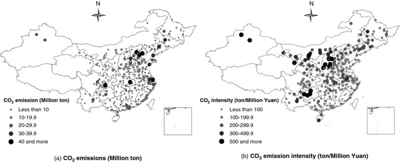
Figure 1. Average Annual CO2 Emissions and Emission Intensity in 287 Cities during 1998 and 2009.
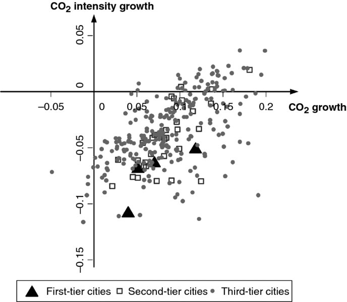
Figure 2. Annual Industrial CO2 Emissions Growth and CO2 Emission Intensity Growth in 287 Cities.
Figure 2 depicts the positions of the 287 cities in terms of their annual growth rates in both total industrial CO2 emissions (X axis) and CO2 emission intensities (Y axis). The annual growth rate of industrial CO2 emissions during this 12-year period is 9.3% for all cities, and 7.4%, 8.9% and 9.4% for the first-tier, second-tier and third-tier cities, respectively. These figures are lower than a recent all sector forecasting exercise by Auffhammer and Carson (2008) based on population projections, which did not account for recent policy intervention and other potential local determinants. Our estimates at the disaggregated city level show that, a large portion of cities locate in the fourth quadrant, enjoying a decline in CO2 emission intensity (composition and technique effects) but experiencing rising industrial CO2 emissions due to the sizable scale effect. The first-tier cities are all in the fourth quadrant, and they are among the cities with the fastest declining CO2 emission intensity. Most of the second-tier cities are also in the fourth quadrant, and they locate at the upper right of first-tier cities, which indicates a relatively higher CO2 emission growth rate but a slower CO2 emission intensity decline compared to the first-tier cities. A large share of the third-tier cities are also in the fourth quadrant, while a small number of cities locate in the first quadrant with growth in both CO2 emission and its intensity. Shizuishan and Yinchuan (both in Ningxia Province) are the top two cities in terms of total CO2 emission growth and CO2 emission intensity growth because of their large share of energy-intensive industries; Beijing ranks at the top in terms of total CO2 emissions decline, thanks to its successful and ongoing transformation to service industries and the vast technical innovations.
Now we turn to our decomposition results. We first look at the national level numbers. Figure 3(a) illustrates the decomposition results for total industrial CO2 emissions at the national level. We first look at the changes between the initial and end years. Arrow ① shows that, if we had held the composition of industries and the production technology constant (Δθ = 0, Δe = 0) during this 12-year period, what the size of the total industrial CO2 emissions would be (the column length between C and F). This scale effect equals to a 221% increase (37 billion tons). Arrow ② measures the composition effect. It is positive, but the size is small (1.3%, 22 million tons in total and 3.03 tons per value-added million Yuan) due to the mix of negative composition effects in some cities but positive effects in other cities. The column length between C and E is what the CO2 emissions would be if every industrial activity still used the production techniques from 1998, which combines the scale and composition effects. Arrow ③ indicates the technique effect, which reduces CO2 emissions. Its size is much larger than that of the composition effect, with contributing to a 41% decrease (690 million tons in total and 97.5 tons per value-added million Yuan) in CO2 emissions from China's urban industrial sector.
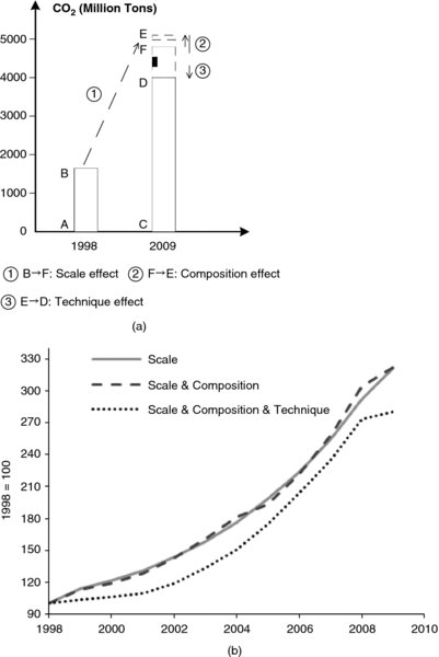
Figure 3. Decomposition Results for Industrial CO2 Emissions at the National Level.
Figure 3(b) plots these three effects at the national level in each of the 12 years. The solid line depicts the pure scale effect (the would-be CO2 emissions in each year if all industries keep the same shares and the same production technology as those in 1998). The middle dashed line plots what CO2 emissions would be in each year if every industrial activity used the original production technique in 1998 (the combination of both scale and composition effects). The gap between the middle dashed and the solid lines shows that the composition effect has led to a smaller change in CO2 emissions between 1998 and 2007 with somewhat rising CO2 emissions in the last two years. The bottom dashed line depicts CO2 emissions when considering all three decomposed effects, so this measures the real CO2 emissions in every year. The gap between this line and the middle dashed line reveals that the technique effect always works to reduce carbon dioxide emissions over time.
For the purposes of this paper we are more interested in the city-level industrial CO2 emissions dynamics. Figure 4(a) shows some interesting patterns in these dynamics. We find the three effects play different roles at the three tiers of cities. The scale effect contributes to the rise of CO2 emissions in all three tiers of cities. The absolute value of this effect is the largest for the first-tier cities and the smallest for the third-tier cities. The technique effect universally leads to the reduction of CO2 emissions for all three tiers, indicating that all cities have enjoyed the improvements in both production technology and management quality. At the same time, the composition effect on CO2 emissions is mild. We find that the composition effect contributes to the rising CO2 emissions in the third-tier cities, while it reduces CO2 emissions in the first-tier and second-tier cities. Figure 4(b) shows the dynamic change in CO2 emission per capita across different tiers of cities between 1998 and 2009. We find that second-tier cities have higher levels of CO2 emissions per capita than the other two. The decomposition patterns using CO2 emissions per capita across these three groups of cities are quite similar to those using total CO2 emission illustrated in Figure 4(a). Our decomposition results suggest that there may be a relocation of those energy-intensive industries from the first-tier and second-tier cities to those third-tier medium- and small-sized cities. In this sense, larger cities enjoy less CO2 emissions at the expense of the increasing emissions in medium- and small-sized cities, so the domestic ‘pollution haven’ does exist. Yet this effect appears to be small.
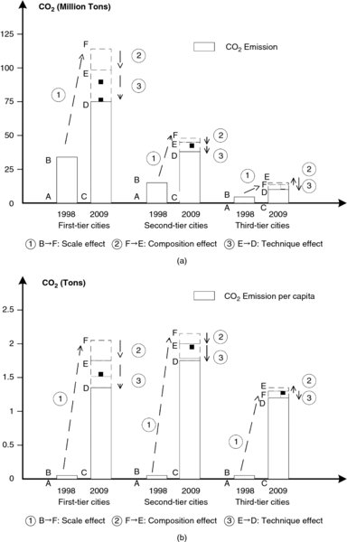
Figure 4. The Decomposition Results of CO2 Emission across Three Tiers of Cities: 1998 versus 2009.
We further examine CO2 emissions changes over time across these three tiers of cities, respectively (See Appendix B). The results show that the increased CO2 emissions in the first-tier cities over the past decade is more attributable to the scale effect, but the composition change towards cleaner industries and the technique improvement helps to offset the otherwise much higher CO2 emissions. The second-tier cities have experienced similar patterns of these three decomposed effects on the change in CO2 emissions but the contribution of composition effect on emission reduction is smaller than in the first-tier cities. In the third-tier cities only the technique effect works to reduce CO2 emissions, but both the scale and composition effects work to increases emissions.
4. The Impacts of FDI and Environmental Regulations on Scale, Composition and Technique Effects
Using the results from Section 3.2.1.3, we are able to examine the impacts of FDI and environmental regulations on these three decomposed effects, and thus gain a better understanding of the underlying mechanisms why such impacts are heterogeneous across cities.
4.1 FDI Measures and Proxies for Environmental Regulation Intensity
4.1.1 FDI and Its Instrumental Variable
We use the ratio of annual foreign direct investment (FDI) in a city's total GDP as the proxy for a city's participation in global trade, which of course is a strong assumption. The city-level data sets on FDI and GDP are from the China's Urban Statistical Yearbooks in the corresponding years. Column (2) in Table 1 illustrates the average ratios of FDI in total GDP for three tiers of cities, respectively. The first-tier cities have received much more FDI compared to the other two tiers of cities.
Table 1. Cross-City Variations in FDI, Industrial Electricity Price and Waste Water Treatment Fee.
| (1) | (2) | (3) | (4) | |
| The ratio of FDI to GDP | Industrial electricity price | Industrial waste water treatment fee (RMB/ton) | Environmental Regulation Index (ERI) (RMB/KWH) (1998–2009) | |
| First-tier cities | 0.85% | 0.46 | 1.14 | 0.37 |
| Second-tier cities | 0.58% | 0.34 | 0.83 | 0.31 |
| Third-tier cities | 0.29% | 0.35 | 0.52 | 0.26 |
When examining the impact of FDI on energy and environmental indicators, a typical challenge a researcher faces is the endogeneity arising from possible reverse causality. If those Chinese cities with more energy-intensive industries impose more regulations and if FDI flows to less regulated areas, then FDI will be pushed to less energy-intensive cities and the OLS estimate will be biased toward finding that FDI lowers CO2 emissions. Conversely, if some cities are clean as they impose more regulation, the OLS estimate will be biased toward finding that FDI increases CO2 emissions (Keller and Arik, 2002). Therefore, we use an IV strategy to overcome this endogeneity issue. Following Zheng et al. (2010), we take advantage of the regional favoritism exhibited by China's government to construct the instrumental variables. Cities on the coast, especially those close to major ports, receive favorable ‘open-door’ development policies from the central government and this encourages greater FDI to flow to these cities. Therefore, we use a city's distance to the closest major port as IV for our FDI measure. This variable is time-invariant so we can only use this to explain the spatial variation in FDI inflows.
4.1.2 Proxies for Environmental Regulations
To measure local officials’ effort in regulating pollution associated with CO2 emissions, we develop an Environmental Regulation Index (ERI) by combining two observable regulation tools at the city level. One is related to the differentiated industrial electricity pricing across cities. In China, as a legacy of communism, the central government has used its power to control energy prices (Tan and Frank, 2009). However, recently the central government is increasingly willing to allow energy prices to fluctuate and decentralize the energy pricing power to the local level, which enables local governments to use energy prices as a policy tool to attract or regulate energy- and pollution-intensive industries. We collect the price of electricity for industrial usage across provinces from China's Price Yearbooks in the corresponding years.11 As shown in Column (3) of Table 1, there is big variation in the electricity price across the three tiers of cities. The other is the industrial sewage treatment fee that firms have to pay. Lan et al. (2011) use this measure to proxy for the stringency of local governments’ pollution regulation. The data on industrial sewage investment is collected from China's Urban Statistical Yearbooks in the corresponding years. Column (4) in Table 1 illustrates the industrial sewage treatment fees in the unit of RMB/ton. The data reveals that first-tier cities in China are likely to put more investment on industrial sewage treatment than the other two groups of cities.
Calculating ERI begins with transforming two city-level environmental regulation indicators, electricity price changes (EPC) and industrial waste water treatment fee (IWWTF), to two standardized and comparable performance scores ranging from 0 to 1 (SCOREEPC and SCOREIWWTF), respectively. ERI for city k is then calculated by averaging the two standardized scores of these two indicators in city k:
In Equation (5), SCOREk = (Zk – L)/(H – L), in which H is the highest level of the indicator, L is the lowest level of the indicator and Zk is the value of the indicator for city k.
Column (5) in Table 1 presents the ERI across cities. It is found that first-tier cities have higher ERI values than that of the other two groups of cities, which is consistent with the statistics of the two individual indicators in Column (3) and (4).
4.2 Estimation Results
We examine the effects of these local factors on the change in carbon dioxide emissions and its three decomposed components using China's city-level data between 1998 and 2009 via a reduced form approach. Equation (6) is in the form of first-difference because the three decomposed effects are with respect to the changes in CO2 emissions. The first-difference specification also enables us to drop out city-level time-invariant unobservables. We also include regional fixed effects to control for region-specific trend in CO2 emissions changes.
We have four versions of the dependent variable ΔYk, including the total changes in CO2 emissions from 1998 to 2009, as well as three decomposed components in city k; ΔFDIk is the change in the share of total GDP for city k between 1998 and 2009; ERIk is city k’s environmental regulation index; X is vector of control variables including the changes in GDP, share of secondary industry in GDP and share of tertiary industry in GDP; rk is regional fixed effects12 and εk is the error term.
Table 2 reports the OLS estimation results and Table 3 provides those with FDI being instrumented with the distance to the closest port. Firstly, we look at the estimated coefficients of the change in our FDI measure (FDI to GDP ratio) using OLS. The coefficient is negative and significant at the 1% level, suggesting that the inflow of FDI pulls down energy intensity and thus CO2 emissions. Specifically, a 10% increase in the FDI to GDP ratio contributes to a 1.74 percentage point decrease in CO2 emissions. As for the three decomposed effects, the estimated coefficient of the change in the FDI measure the technique effect is significantly negative, while the estimates on the other two effects are insignificant. These suggest that the inflow of FDI works on pollution emission more through the technique effect than the scale effect. This justifies why we find the optimistic result that FDI helps a city to reduce CO2 emissions (and corresponding energy consumption). The underlying reasons may be that FDI brings in cleaner capital, technology and better management skills. As the IV estimation results suggest (see Table 3), the inflow of FDI reduces CO2 emissions, but with larger magnitudes in terms of its impact on the total CO2 emission change and the change of the technique component compared with OLS estimates. A 10% increase in the FDI to GDP ratio leads to a 6.89 percentage point decrease in total CO2 emissions and a 4.31 percentage point decrease in CO2 emissions due to the technique effect. This finding is consistent with our statistical analysis in Table 1 that the cities with more FDI also impose more regulation on the environment.
Table 2. Effects of FDI and Environmental Regulations on CO2 Emissions and the Three Decomposed Effects (OLS).
| (1) | (2) | (3) | (4) | |
| ΔCO2 | Scale | Composition | Technique | |
| emissions | effect | effect | effect | |
| ΔLog(FDI) | –0.174*** | –0.009 | –0.005 | –0.053** |
| (0.045) | (0.036) | (0.011) | (0.022) | |
| ERI | –1.981*** | –1.191*** | –0.262** | –0.527** |
| (0.473) | (0.338) | (0.114) | (0.205) | |
| ΔLog(GDP) | 1.698*** | 2.278*** | –0.117** | –0.422*** |
| (0.210) | (0.143) | (0.0513) | (0.093) | |
| ΔSecondary Industry GDP Share | 0.055*** | 0.032*** | 0.030*** | –0.011 |
| (0.010) | (0.008) | (0.00251) | (0.016) | |
| ΔTertiary Industry GDP Share | 0.002 | 0.0158* | 0.005 | –0.019*** |
| (0.013) | (0.009) | (0.00318) | (0.006) | |
| Constant | –0.217 | –0.725*** | 0.023 | 0.442*** |
| (0.299) | (0.212) | (0.0714) | (0.128) | |
| Region fixed effects | Yes | Yes | Yes | Yes |
| Observations | 186 | 186 | 186 | 186 |
| R2 | 0.603 | 0.721 | 0.641 | 0.329 |
Note: Standard errors are reported in parentheses, which are clustered by province. *p < 0.10, **p < 0.05, ***p < 0.01.
Table 3. Effects of FDI and Environmental Regulations on CO2 Emissions and the Three Decomposed Effects (Using IV for FDI).
| (1) | (2) | (3) | (4) | |
| ΔCO2 | Scale | Composition | Technique | |
| emissions | effect | effect | effect | |
| ΔLog(FDI) | –0.689*** | –0.076 | 0.024 | –0.431* |
| (0.241) | (0.435) | (0.045) | (0.231) | |
| ERI | –1.729*** | –0.899** | –0.269** | –0.435 |
| (0.623) | (0.405) | (0.113) | (0.332) | |
| ΔLog(GDP) | 1.533*** | 2.298*** | –0.109** | –0.502*** |
| (0.281) | (0.243) | (0.053) | (0.155) | |
| ΔSecondary Industry GDP Share | 0.057*** | 0.055*** | 0.030*** | 0.001 |
| (0.014) | (0.020) | (0.002) | (0.010) | |
| ΔTertiary Industry GDP Share | –0.010 | 0.019 | 0.005 | –0.019** |
| (0.018) | (0.016) | (0.003) | (0.009) | |
| Constant | 0.018 | –0.425 | –0.063 | 0.669** |
| (0.495) | (0.482) | (0.091) | (0.300) | |
| Region fixed effects | Yes | Yes | Yes | Yes |
| Observations | 186 | 186 | 186 | 186 |
| R2 | 0.591 | 0.738 | 0.627 | 0.420 |
Note: Standard errors are reported in parentheses, which are clustered by province. *p < 0.10, **p < 0.05, ***p < 0.01.
In Table 3, as expected, the Environmental Regulation Index has a negative impact on industrial carbon emissions. If we look into the three decomposed effects, we can see that stringent environmental regulation works through all three channels – the scale of production drops, the industrial composition shifts towards cleaner industries, and the production technology and management quality also increase (a significant negative technique effect). The magnitudes of the three coefficients suggest that the scale effect dominates this process. The observed composition effect due to the enforcement of environmental regulations is consistent with those in previous studies in the USA such as Berman and Bui (2001a, 2001b) and Henderson (1996). As the instrumental variable strategy here is less than perfect due to the lack of time series variation in the instrument, these results should be taken as suggestive.
The estimated coefficients on the other control variables are also consistent with our expectations. Cities with higher GDP growth experience a larger increase in CO2 emission mainly due to the increases in economic scale, which dominates the changes from cleaner industry composition and more efficient production technology. The growth in the share of secondary industry is found to increase the cities’ CO2 emission through scale and composition effect, while the growth of tertiary industry helps to decrease CO2 emission by improving production technology.
We are also interested in whether the effect of FDI and environment regulation on CO2 emissions varies across these three tiers of cities. We estimate Equation (6) separately for the first, second-tier cities and third-tier cities, and the regression results are provided in Table 4. It shows that the change in FDI had insignificant effect on CO2 emissions in the first and second-tier cities, while it tends to decrease CO2 emissions in the third tier cities mainly through the technique effect. A possible explanation is that the first- and second-tier cities already have advanced technologies (in our study period) so the marginal effect of FDI is weak; while its marginal effect is much larger in the third tier cities where production technologies stand at a lower level. Stringent environmental regulation is found to contribute to the declining CO2 emission in all three groups of cities. This mitigation effect is mostly attributed to the technique effect in the first- and second-tier cities, while to the scale and composition effects in the third-tier cities. Our results indicate that the environmental regulation in the first- and second-tier cities helps to promote the adoption of greener production technology, but it constrains the scale expansion and the receipt of dirty industries (relocating from the first and- second-tier cities) in the third-tier cities.
Table 4. Effects of FDI and Environmental Regulations on CO2 Emissions in Different Cities (Using IV for FDI).
| (1) | (2) | (3) | (4) | |
| ΔCO2 emissions | Scale effect | Composition effect | Technique effect | |
| First- and second-tier cities | ||||
| ΔLog(FDI) | –1.173 | –1.174 | –0.090 | 0.140 |
| (0.940) | (0.815) | (0.121) | (0.192) | |
| ERI | –3.453* | –1.394 | 0.116 | –1.473*** |
| (2.090) | (1.768) | (0.270) | (0.503) | |
| Third-tier cities | ||||
| ΔLog(FDI) | –0.656** | –0.082 | –0.024 | –0.567** |
| (0.265) | (0.349) | (0.049) | (0.226) | |
| ERI | –1.425** | –1.050*** | –0.291** | –0.145 |
| (0.643) | (0.338) | (0.115) | (0.474) | |
Note: Standard errors are reported in parentheses, which are clustered by province. Other specifications are same with those of Table 3. *p < 0.10, **p < 0.05, ***p < 0.01.
5. Conclusions
In 2007, China became the largest greenhouse gas emitter in the world. 85% of China's GHG emissions are attributed to urban economic activities, and this share will continue to increase with China's rapid urbanization process. This paper enriches our understanding of city-level industrial CO2 emissions in China and its dynamics by decomposing CO2 emission changes into scale, composition and technique effects over the past decade (all 287 prefecture-level-cities in 1998–2009).
The paper first reviews the literature on the decomposition analysis and several local determinants that shape such dynamics. We then use city-level data in China to decompose the changes in industrial CO2 emissions into the scale, composition and technique effects. Our estimates show that the industrial CO2 emissions per capita are about 3.4 times larger than the residential CO2 emissions per capita in China's urban sector and the industrial CO2 emissions have been increasing by 9.3% annually during this 12-year period. The decomposition analysis shows that the three effects play different roles in the three tiers of cities. The scale effect contributes to the rise of CO2 emissions in all cities. On the other hand, the technique effect universally leads to the reduction of CO2 emissions in all three tiers of cities, indicating that all cities have enjoyed the improvements in both production technology and management quality towards energy efficiency. The composition effect on CO2 emissions is mild – it contributes to the rising CO2 emissions in the third-tier cities, while it reduces CO2 emissions in the first-tier and second-tier cities. These patterns suggest that there may be a relocation of those energy-insensitive industries from the first-tier and second-tier cities to those third-tier medium- and small-sized cities. In this sense, larger cities enjoy less CO2 emissions at the expense of the increasing emissions in medium- and small-sized cities.
Our decomposition results facilitate us to provide some suggestive evidence as to how FDI inflow and environmental regulations drive the change in CO2 emissions and its decomposed three effects. It is found that the inflow of FDI pulls down energy intensity and thus CO2 emissions by generating significant technique effect (and the other two effects are insignificant), so it brings in cleaner production technology and better management quality. The environmental regulations help cities to reduce their industrial CO2 emissions through all three channels –the economy scale shrinks, the industrial composition shifts towards cleaner industries and the energy-efficient technologies and management skills also improve.
Our empirical results clearly indicate that shifting towards less-energy-intensive industries (composition effect), exploiting ‘clean’ fuel inputs and fostering technology transfers (technique effect), matter for China in curbing carbon dioxide emissions during its ongoing urbanization and industrial progress. The Chinese government has pledged to wean its economy away from reliance on fossil fuels as it grows. In November 2014, China and the US unveiled new pledges on greenhouse gas emissions. The deal commits China to reducing greenhouse gas emissions after a peak in 2030 (and ideally sooner). China also aims to have non-fossil fuels make up 20% of its primary energy consumption by 2030. It is the first time China, the world's largest emitter by far in absolute terms (roughly 28% of the world's CO2 emissions in 2014), has agreed to set a ceiling, albeit an undefined one, on overall emissions. To achieve this goal, the central government in China will come up with ways of incentivizing local officials to go green, and city mayors will make their own trade-off between their economic growth (scale), and environmental goals (economic restructure and technology improvements). The decomposition framework in our paper can help policy makers and scholars to observe such trade-offs and the underlying rationales.
Acknowledgements
We deeply appreciate anonymous referees for their insightful comments. Weizeng Sun and Siqi Zheng thank the National Natural Science Foundation of China (No. 71273154, No. 71322307, No. 71533004) and the Key Project of National Social Science Foundation of China (No. 13AZD082), and Volvo Group in a research project of Tsinghua University's Research Center for Green Economy and Sustainable Development for research support. Jianfeng Wu thanks the School of Economics at Fudan University for granting us access to key data. He thanks the MOE Project of the Key Research Institute of the Humanities and Social Sciences at the China Center for Economic Studies (CCES), and the Research Institute of Chinese Economy (RICE) at Fudan University. He also thanks the National Natural Science Foundation of China (No. 71573054).
Notes
References
- Antweiler, W., Copeland, B. and Taylor, M. (2001) Is free trade good for the environment? American Economic Review 91: 877–908.
- Auffhammer, M. and Carson, R.T. (2008) Forecasting the path of China's CO2 emissions using province level information. Journal of Environmental Economics and Management 55(3): 229–247.
- Auffhammer, M. and Gong, Y. (2015) China's Carbon Emissions from fossil fuels and market based opportunities for control. Annual Review of Resource Economics 7: 11–34.
- Becker, R. and Henderson, J.V. (2000) Effects of air quality regulations on polluting industries. Journal of Political Economy 108(2): 729–758.
- Berman, E. and Bui, L.T.M. (2001a) Environmental regulation and labor demand: Evidence from the South Coast Air Basin. Journal of Public Economics 79(2): 265–295.
- Berman, E. and Bui, L.T.M. (2001b) Environmental regulation and productivity: Evidence from oil refineries. Review of Economics and Statistics 83(3): 498–510.
- Bloom, N., Genakos, R., Martin, R. and Sadun, R. (2010) Modern accounting: Good for the environment or just hot air? Economic Journal 120: 551–572.
- Brandt, L., Biesebroeck, J. V. and Zhang, Y. (2012) Creative accounting or creative destruction? Firm-level productivity growth in Chinese manufacturing. Journal of Development Economics 97(2): 339–351.
- Bustos, P. (2011) Trade liberalization, exports and technology upgrading: Evidence on the impact of MERCOSUR on Argentinean firms. American Economic Review 101(1): 304–340.
- Cai, F., Chen, Y. and Qing, G. (2016) Polluting thy neighbor: The case of river pollution in China. Journal of Environmental Economics and Management 76: 86–104.
- Copeland, B.R. and Taylor, M.S. (1994) North-south trade and the environment. Quarterly Journal of Economics 109(3): 755–787.
- Copeland, B.R. and Taylor, M.S. (2003) Trade and the Environment: Theory and Evidence. Princeton: Princeton University Press.
- Copeland, B.R. and Taylor, M.S. (2004) Trade, growth, and the environment. Journal of Economic Literature 42(1): 7–71.
- Creutzig, F., Baiocchi, G., Bierkandt, R., Oichler, P.-P. and Seto, K.C. (2013) Global typology of urban energy use and potentials for an urbanization mitigation wedge. Proceedings of the National Academy of Science of the United States of America 112(20): 6283–6288.
- Cui, H., Lapan, H. and Moschini, G. (2012) Are exporters more environmentally friendly than non-exporters? Theory and evidence. Working paper No.12022, Department of Economics, Iowa State University.
- Dean, J.M. (2002) Does trade liberalization harm the environment? A new test. Canadian Journal of Economics 35(4): 819–842.
- Fisher-Vanden, K., Jefferson, G.H., Liu, H. and Tao, Q. (2004) What is driving China's decline in energy intensity? Resource and Energy Economics 26: 77–97.
- Greenstone, M. (2002) The impacts of environmental regulations on industrial activity: Evidence from the 1970 and 1977 Clean Air Act Amendments and the Census of manufacturers. Journal of Political Economy 110(6): 1175–1219.
- Grossman, G.M. and Krueger, A.B. (1995) Economic growth and the environment. Quarterly Journal of Economics 110(2): 353–377.
- He, J. (2006) Pollution Haven Hypothesis and environmental impacts of Foreign Direct Investment: The case of industrial emission of sulfur dioxide (SO2) in Chinese provinces. Ecological Economics 60(1): 228–245.
- He, J. (2009) China industrial SO2 emissions and its economic determinants of EKC's reduced vs. structural model and the role of international trade. Environmental and Development Economics 14(2): 227–262.
- Henderson, J.V. (1996) Effects of air quality regulation. American Economic Review 86(4): 789–813.
- Kahn, M.E. (1997) Particulate pollution trends in the United States. Regional Science and Urban Economics 27(1): 87–107.
- Kahn, M.E. and Mansur, E.T. (2013) Do local energy prices and regulation affect the geographic concentration of employment? Journal of Public Economics 101: 105–114.
- Keller, W. and Arik, L. (2002) Pollution abatement costs and foreign direct investment inflows to US states. Review of Economics and Statistics 84(4): 691–703.
- Kreickemeier, U. and Richter, P.M. (2014) Trade and the environment: The role of firm heterogeneity. Review of International Economics 22(2): 209–225.
- Jiang, L., Lin, C. and Lin, P. (2014) The determinants of pollution levels: Firm-level evidence from Chinese manufacturing. Journal of Comparative Economics 42(1): 118–142.
- Lan, H., Livermore, M.A. and Wenner, C.A. (2011) Water pollution and regulatory cooperation in China. Cornell International Law Journal 44(2): 349–383.
- Lin, L. (2013) Enforcement of pollution levies in China. Journal of Public Economics 96: 32–43.
- Lin, S.J. and Chang, T.C. (1996) Decomposition of SO2, NOX and CO2 emissions from energy use of major economic sectors in Taiwan. Energy Journal 17(1): 1–17.
- Liu, Z. (2015) China's Carbon Emission Report 2015. Belfer center for science and international affairs, Harvard Kennedy School.
- Ma, C. and Stern, D.I. (2008) China's changing energy intensity trend: A decomposition analysis. Energy Economics 30: 1037–1053.
- Martin, L.A. (2011) Energy efficiency gains from trade: Greenhouse gas emissions and India's manufacturing sector. Mimeography, Berkeley ARE.
- Managi, S., Hibiki, A. and Tsurumi, T. (2009) Does trade openness improve environmental quality? Journal of Environmental Economics and Management 58: 346–363.
- Melitz, M.J. (2003) The impact of trade on intra-industry reallocations and aggregate industry productivity. Econometrica 71(6):1695–1725.
- OECD (2015) Urban Policy Review: China 2015. Available at http://www.oecd.org/china/oecd-urban-policy-reviews-china-2015-9789264230040-en.htm. (accessed on April 18, 2015).
- Sinton, J.E., and Levine, M.D. (1994) Changing energy intensity in Chinese industry: The relative importance of structural shift and intensity change. Energy Policy 22: 239–255.
- Shapiro, J.S. and Walker, R. (2015) Why is pollution from U.S. manufacturing declining? The roles of trade, regulation, productivity, and preferences. NBER Working Paper No. 20879.
- Tan, X. and Frank, W. (2009) Does China underprice its oil consumption? Working Paper. Department of Economics, Stanford University.
- Van Rooij, B. and Lo, C.W. (2010) Fragile convergence: Understanding variation in the enforcement of China's industrial pollution law. Law and Policy 32(1): 14–37.
- Viguier, L. (1999) Emissions of SO2, NOX and CO2 in transition economies: Emissions inventories and Divisia index analysis. Energy Journal 20(2): 59–87.
- Wang, H. and Wheeler, D. (2005) Financial incentives and endogenous enforcement in China's pollution levy system. Journal of Environmental Economics and Management 49: 174–196.
- Wang, S., Fang, C., Guan, X., Pang, B. and Ma, H. (2014) Urbanization, energy consumption, and carbon dioxide emissions in China: A panel data analysis of China's provinces. Applied Energy 136: 738–749.
- Wang, H. and Jin, Y. (2007) Industrial ownership and environmental performance: Evidence from China. Environmental and Resource Economics 36(3): 255–273.
- Xu, B. and Lin, B. (2015) How industrialization and urbanization process impacts on CO2 emissions in China: Evidence from nonparametric additive regressions models. Energy Economics 48: 188–202.
- Xu, Y., Williams, R.H. and Socolow, R.H. (2009) China's rapid development of SO2 scrubbers. Energy and Environmental Science 2(5): 459–465.
- Yu, J., Zhou, L. and Zhu, G. (2013) Strategic interaction in political competition: Evidence from spatial effects across Chinese cities. Working paper.
- Zhang, Y. (2012) Scale, technique and composition effects in trade-related carbon emissions in China. Environment and Resource Economics 51: 371–389.
- Zheng, S. and Kahn, M. E. (2013) Understanding China's urban pollution dynamics. Journal of Economic Literature 51(3): 731–772.
- Zheng, S., Kahn, M.E. and Liu, H. (2010) Towards a system of open cities in China: Home prices, FDI flows, and air quality in 35 major cities. Regional Science and Urban Economics 40(1): 1–10.
- Zheng S., Kahn, M.E., Sun, W. and Luo, D. (2014) Incentivizing China's urban mayors to mitigate pollution externalities: The role of the central government and the public environmentalism. Regional Science and Urban Economics 47: 61–71.
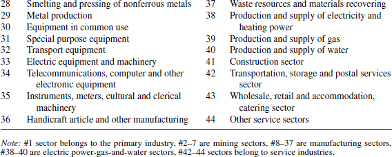
Appendix A
List of 44 Sectors/Subsectors

Appendix B
Decomposition Effects of CO2 Emissions for Three-Tier Cities from 1998 to 2009
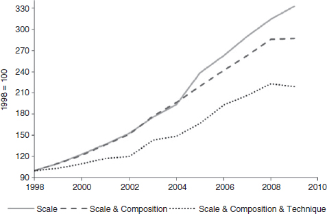
Figure A1. Decomposition Effects of CO2 Emission for First-Tier Cities from 1998 to 2009.

Figure A2. Decomposition Effects of CO2 Emission for Second-Tier Cities from 1998 to 2009.
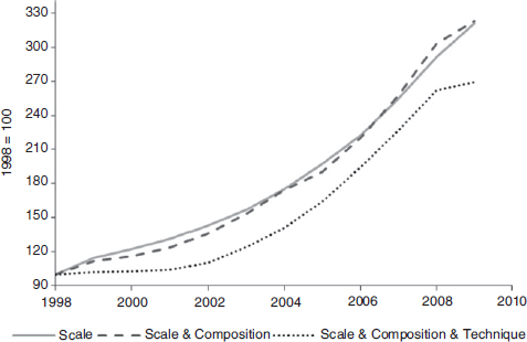
Figure A3. Decomposition Effects of CO2 Emission for Third-Tier Cities from 1998 to 2009.