
3
STRUCTURAL EQUATION MODELLING AND THE CAUSAL EFFECT OF PERMANENT INCOME ON LIFE SATISFACTION: THE CASE OF AIR POLLUTION VALUATION IN SWITZERLAND
Eleftherios Giovanis
Verona University
Oznur Ozdamar
Adnan Menderes University and Bologna University
1. Introduction
Air pollution has harmful effects on human health and ecosystems. Thus, it can also impact the Earth's climate. It is well known that pollutants released into the atmosphere not only cause local air pollution, but they also cause regional air pollution, such as acid rain and huge plumes of smoke covering large areas. The high levels of pollutants are more harmful in causing global environmental problems, as ozone depletion and climate change. Especially, O3 and SO2 contribute to global warming which is linked to climate change.
Air pollution also has significant negative impact on well-being, such as life satisfaction and health status. It is, therefore, crucial to have reliable estimates of the public willingness-to-pay for air pollution reduction. Overall, there are mainly three popular methods for the environmental valuation that are revealed preference, stated preference and the life satisfaction approach.
Revealed preference relies on hedonic price analysis, that is, uses variations in house price to elucidate the price attached to a cleaner environment. This approach has some limitations, such as it requires the market of interest (typically the housing market) to be in equilibrium at even small geographical level (Frey et al., 2010), the cost of migration is not considered (Bayer et al., 2009) in the approach and the consumption of the public good examined is detectable (Rabin, 1998), which is the air pollution in our case.
The second approach is the stated preference, which is based on contingent valuation from surveys, and attempts to directly elucidate the environmental value from questions presented to the respondents (Carson et al., 2003). The drawbacks of this approach include the superficial and misleading answers by the respondents due to the hypothetical nature of the surveys or the lack of financial implications (Kahneman et al., 1999).
The third approach is the life satisfaction approach (LSA). One of the main advantages of this method is that it does not rely on how the people directly evaluate the environmental conditions, as in the case of the stated preference approach, neither it requires the housing market to be on equilibrium, as it is the main assumption of the revealed preference approach. Instead individuals are asked to evaluate their general life satisfaction controlling for pollution, income and other socio-economic and weather factors. In the LSA the perception of causal relationships is not required, as it is assumed that air quality leads to life satisfaction changes. Previous research studies examined the relationship between life satisfaction, income and air pollution (Luechinger, 2009; Levinson, 2012).
Nevertheless one important disadvantage of the LSA is the plausible reverse causality between income and life satisfaction, as happier people can be more productive and earn more (Powdthavee, 2010). Overall, Stutzer and Frey (2012) suggest that instrumental variable approaches are hardly convincing. This is because almost every factor can determine the life satisfaction. In line with the previous issue, another common limitation of the LSA is the small estimated income coefficients. This is explained by the fact that individuals compare their current income with their past income, as well as, with their peers’ income, indicating that both relative and absolute income can be important (Ferreira and Moro, 2010; Levinson, 2012). Tsui (2014) examined the effects of income on happiness in Taiwan. The results support that people are happier not only with changes in absolute income, but also with changes related to the expected and relative income.
Although there are disadvantages of LSA approach as stated preferences and revealed preferences also have, due to its comparative advantages, it is the most appropriate approach to analyse the link between life satisfaction, income and air pollution. It is the reason we use it in our study as previous studies also did that focus on analysing a similar relationship.
However, there are significant contributions of this study compared to many others. First, the relevant analysis relies on detailed micro-level data, using SHP's respondents’ zip municipality codes, which allows for mapping the air pollution to individuals more accurately, than previous studies did, where the geographical level was larger (Welsch, 2002, 2006; Luechinger, 2009, 2010; Ferreira and Moro, 2010; Levinson, 2012; Ferreira et al., 2013). Secondly the sample is split to the non-movers and the movers. This can allow to reduce the endogeneity coming from the residential sorting, where the respondents choose where to reside. Thus, those who are more averted to air pollution they will choose locations with cleaner air, resulting to biased air coefficients downwards. Similarly, Luechinger (2009), explored the non-movers and the individuals who are moving across the boundaries of the counties were excluded. In this way, the individual specific fixed effects absorb the county specific effects. Additionally, the air pollution is taken based on daily values, making it more exogenous and avoiding the above-mentioned sorting problem. However, one important issue of the study by Luechinger (2009) and our study is that the sorting process is not observed, as those who are more averted to air pollution have decided to choose locations with clean air and those who are less averted have moved to more polluted areas before the surveys take place. Therefore, as it is pointed out by Luechinger (2009), individuals might become accustomed to the air pollution if they are less sensitive to it, or they might sort into polluted areas at the first place if they are less concerned about air quality. Therefore, for this reason the estimates will take place for both non-movers and movers. On the other hand, people might sort into polluted areas not because are less concerned, but because there might be more opportunities make them happier such as labour market choices. Usually cities are more polluted because of the traffic; nevertheless, cities and urban areas offer opportunities of proximity, a variety of labour and health services choices, which are mainly centralised.
The aim of the paper is to examine the determinants of life satisfaction and to propose a theoretical model where permanent income is considered as one of the important determinants of life satisfaction which cannot be measured directly. However, the impossibility or difficulty to measure abstract variables, such as the permanent income and life satisfaction can be overcome using SEM since it treats them as latent variables, controlling for confounding effects as measurement error. Furthermore, SEM enables a researcher to test a set of regression equations simultaneously. Thus, the main advantage of SEM is to construct a model that combines the determinants of life satisfaction with the permanent income. The concept of permanent income was proposed by Friedman (1957) and is one of the most important developments in empirical social sciences. The model is based on the hypothesis that permanent income might be more important factor on life satisfaction and common proxies for permanent income which most closely capture the concept are examined. In addition, SEM is suggested as it is a more flexible statistical model which allows for measurement error in the income. For the robustness check and to examine the causal effects of permanent income on life satisfaction, and then to calculate the MWTP values, a simple fixed effects regression will also be analysed along with a panel structural equation model (SEM). In order to do that, a model that relates the components of socioeconomic factors and permanent income to life satisfaction is formulated. The results from fixed effects regression analysis show that the MWTP values expressed in 2013 US dollar prices are $8,900, $11,995, $6,580, $1,940, $2,320 for one standard deviation reduction in ozone (O3), sulphur dioxide (SO2), nitrogen dioxides (NO2), carbon monoxide (CO) and particulate matter less than 10 microns (PM10), respectively. On the other hand, employing the SEM the respective values of MWTP values are lower and equal at $6,710, $9,876, $5,390, $1,930 and $2,135. The structure of the paper has as follows: In the next section a brief literature review on the previous environmental valuation approaches is discussed. In Section 3, the methodology and data are presented, while in Section 4 the empirical results are reported. Finally, the concluding remarks are discussed in the last section.
2. Literature Review
Initially, previous researches on revealed preference methods are presented. Under the assumption of perfectly competitive housing market, a change in any environmental characteristics is reflected by a change in market price, and reflects the buyers’ marginal willingness-to-pay (MWTP) for this characteristic; see Rosen (1974) for details on hedonic pricing. One of the first studies that employed the hedonic pricing method is by Ridker and Henning (1967), who estimated that a one standard deviation change in sulphate leads to a 2.8% change in the values of residential properties. Numerous studied followed the same methodology and are reviewed in Smith and Huang's (1995) meta-analysis. However, this method is subject to a number of criticism, such as the study by Bayer et al. (2009), who show that when moving is costly, estimates relying on hedonic valuation of the housing market are biased downwards. The form can be another issue as Kuminoff et al. (2010) point out where a framework incorporating quasi-experimental identification and spatial fixed effects can be more flexible than the standard linear specifications.
In the literature three main sorting and hedonic pricing models have additionally been developed in order to improve the estimates; the Pure Characteristics (PC) sorting, the Random Utility (RU) sorting and the Calibrated Sorting (CS) models. The differences in these models include: the set of choices faced by each household; the shape of the preference function specification and the development of instruments to control for endogenous amenities (Bayer and Timmins, 2005, 2007; Kuminoff et al., 2013).
Regarding preferences in the PC specification, every household is required to have for every amenity the same relative preferences, while the specification in the CS allows the households to differ in their relative preferences relaxing in this way the illustration of preference heterogeneity. In the PC model, the vertically differentiated case dominates where the households agree on the community ranking by the provision of a public good or amenity and on the spatial substitution opportunities. On the other hand, in the CS and RU models the horizontal differentiation condition applies, where a broader diversity in the substitution possibilities is allowed. However, there is a bias/variance trade-off in the vertical/horizontal modelling. The PC estimator is biased by the vertically differentiated condition leading to biased conclusions on welfare measures. On the contrary, the restriction that creates bias is removed by the horizontal differentiation, but untested distributional assumptions are created due the dimensions of preferences which are added in the modelling which drive the estimates (Kuminoff et al., 2013). In the case of the instrumental variable approach and the CS model, the assumption about the relative importance of unobserved amenities is not required as it has been illustrated by Ferreyra (2007) and Calabrese et al. (2007). The instruments employed in the PC model are constructed using the ranking of the community income functions, while in the RU sorting model the instruments are developed by the functions of the exogenous attributes of substitute locations (Kuminoff et al., 2013). Nevertheless, there are still drawbacks as the instrumental variable approaches employed in the PC and RU model will be consistent as long as the instruments are valid, that is, exogenous and not weak, while a specific form of the amenity's production function is required in CS model (Kuminoff et al., 2013).
Furthermore, the previous research studies using stated preference methods are discussed. Contingent evaluation studies are difficult to compare because each study is unique and it depends on the description of the good to be evaluated; the payment method to be made; and the eliciting values method (Croper and Oates, 1992, 710). The study by Loehman and De (1982) shows that the yearly MWTP values range between US $7 and $46 for a one-day per year reduction in severe cough, severe shortness of breath, and minor eye irritation. Hall et al. (1992) found that the MWTP value per day for a one-day-per-year reduction in minor restricted-activity is equal at US $23 deflated at 1990 prices. Hammitt and Zhou (2006) using the contingent valuation method, explored the indoor pollution and specifically the PM10 and SO2. The authors found that the statistical cost of a cold, chronic bronchitis and the value per statistical life range, respectively, between $3 and $6, $500 and $1,000 and $4,200 and $16,900 based on 2000 prices. The stated preference approach has been subject of criticism on two main points. Firstly, the individuals have not always adequate understanding of the good they are asked to evaluate. Second, a major disadvantage is the strategic behaviour or the limited incentives given to respondents, resulting to disclosure of their true demand. The consequence is that the estimates will be biased since the respondents give misleading answers (Luechinger, 2009; MacKerron and Mourato, 2009; Frey et al., 2010).
However, other studies used the approaches of the choice modelling (CM) or choice experiments (CEs) suggesting that these can be more proper than the contingent valuation in order to calculate the MWTP (Hanley et al., 2001a; Campbell, 2007; Campbell et al., 2008). These type of experiments are based on survey methodology to model the preferences for goods, which are described regarding their attributes and levels. Furthermore, the alternative series of preferences are provided to the respondents, which differ in levels and terms and then they are asked to choose the most preferred one or to rank the pool of alternatives. In the next step, the price or cost is concluded as one of the goods’ attributes which allows to recover indirectly the respondent's choices or rankings (Hanley et al., 2001a; Campbell et al., 2011). In addition, it is suggested that CE approach can be more enlightening than the studies, using the discrete CV approach, since the respondents can choose or express their preference for a specific good given a range of payment amounts. Finally, CE approach relies on the respondents'ranking ratings among a series of alternative packages that the MWTP can be indirectly calculated, avoiding or minimising the strategic behaviour commonly presented in the CV approach (Hanley et al., 2001a; Campbell et al., 2011).
Nevertheless, CEs have also weakness. One drawback is the statistical problems derived from the repeated answers for each respondent, as well as, the correlation among the responses should be considered (Adamowicz et al., 1998). In addition, the study design in CE modelling can be sensitive, as the estimates depend on the way that the choice of the levels to represent them are selected and the way that the respondents receive them are neutral or not. This implies that there might be an impact on the marginal utilities values (Hanley et al., 2001a, 2001b) found that the respondents are affected from the way that the choices are given to them. Changing the number of choice tasks has a significant impact on the respondent's preferences.
To alleviate the dependence on the housing market and to evaluate the willingness-to-pay, researchers have also used life satisfaction. Welsch (2002) explored 54 countries in 1990 and 1995, using cross sectional data, where the dependent variable is the country average happiness. MWTP is found to be $126 for a 1 μg/m3 decrease in nitrogen dioxide (NO2). In another study, Welsch (2006) employed a series of the Eurobarometer cross-sectional survey during the period 1990–1997 for 10 European countries. The MWTP was found equal at $184 and $519 for 1 μg/m3 decrease, respectively, in lead (Pb) and NO2. However, these studies are likely to be biased by measurement error due to the aggregation of pollution to national level. To reduce this aggregation problem, Ferreira and Moro (2010) used a micro-level data the Irish National Survey on Quality of Life which took place in 2001. The authors found that the MWTP to pay for a reduction of 1 μg/m3 of PM10 is €945. Rehdanz and Maddison (2008) found that the air pollution levels in Germany have negative relationship with life satisfaction. The estimates in previous studies, such as those by Ferreira and Moro (2010) and MacKerron and Mourato (2009) are based on cross-sectional data and do not account for the endogeneity of pollution. For instance, areas with high pollution levels are likely to also have some other amenities that negatively affect life satisfaction. The most relevant paper to our study is by Luechinger (2009) who also uses an individual level panel data (the German Socio-Economic Panel (GSOEP). Luechinger (2009) used as an instrumental variable for SO2 the mandated installation of scrubbers at power plants and he found that the MWTP is $313, while it becomes smaller ($183) when no instrument is considered.
SEM has been previously applied on life satisfaction studies. Powdthavee and Wooden (2015) used SEM in order to examine the effects of sexual identity on life satisfaction through seven channels: income, employment, health, partner, relationships, children, friendship networks and education in Australia and the United Kingdom. Generally, the SEM has not been applied on the valuation of air pollution using the LSA. This study contributes to the previous literature by three ways. First, by mapping air pollution concentrations on municipality zip code level and conventional fixed effects estimates for five air pollutants. Second, SEM approach is expanded including additionally the air pollutants. Third, permanent income is incorporated in the analysis. Overall, SEM enables a researcher to test a set of regression equations simultaneously. Thus, the main advantage of SEM is to construct a model that combines the determinants of life satisfaction with income. Thus, using SEM both the direct and indirect effects of variables such as age or marital status among others can be simultaneously considered. For example, in the analysis of life satisfaction it is important to separate the direct effect of some variables, that is, education from their indirect effect, for example, via its effect on income. In addition, it is impossible to disentangle these factors in a single equation model in which the reduced form parameters include both the direct and indirect effects. SEM approach can entail this.
3. Methodology
3.1 Fixed Effects
The panel data model estimated is
where LS denotes the life satisfaction for individual i in location (zip code) j and in time t, log(y) is the logarithm of the equivalent household income deflated in 2012 prices and e is the air pollution measured-in that case five air pollutants. Vector Ζ includes personal and household characteristics, while W includes the weather conditions. Set μi is the individual fixed effects, Mj is the location fixed effects and set θt is a time-specific vector of indicators for the day of the week, month and the year of the survey. In addition, the regressions control for MjT which is a set of area-specific time trends. Standard errors are clustered at the area-specific time trends. For cross-sectional data or panel data random effects analysis the ordered Probit and Logit models can be applied. However, these models do not allow fixed effects estimation analysis. In this case the approach developed by van Praag and Ferrer-i-Carbonell (2004) is applied, the ‘Probit-adapted’ method, where the dependent variable is transformed to a standardised continuous variable, which is normally-distributed. For a marginal change of air pollutant e, the MWTP can be derived by differentiating (1) and setting dLS = 0. That is the income drop that would lead to the same reduction in life satisfaction than an increase in pollution. Thus, the MWTP can be calculated as
Then the MWTP (2) is multiplied by the average household income in order to get the MWTP values. The within-person estimations achieved with the panel data fixed effects are useful when it is difficult to measure unobserved confounders including determinants of location selection. These are most appropriate for exposure (air pollution) and outcome (life satisfaction) relationships with short lag times as is the case of the current study. Cross-sectional studies exploring the relationship between well-being and air pollution are particularly liable to residential self-selection bias resulted from unmeasured area selection factors. Nevertheless, fixed effects even if they will greatly reduce the potential bias coming from omitted variables, this bias is not completely eliminated, since there might still be unobservable factors driving air pollution and which are correlated with the life satisfaction. Regarding the sample selection, usually residential relocation is triggered by events such as employment changes and marriage which may influence life satisfaction and thus restricting the sample to the movers may induce selection bias (Hernan et al., 2004). Using panel data, the area fixed effects for the non-movers will be eliminated, while in the case of the movers the error term will contain the difference in the area fixed effects of the two residences which is likely to be correlated with the difference of the air pollution levels across the two locations.
However, as it has been mentioned in the introduction section the limitation of the sample to the non-movers may reduce the endogeneity from the residential sorting but it does not account for issues coming from the sorting process. In particular, individuals who are averted to air pollution have already lived or moved to locations with cleaner air before the implementation of the surveys. Thus, similarly to the study by Luechinger (2009) the sorting process is not observed and this might have an effect on the estimated coefficients. Thus, restricting the sample only to the non-movers the above selection bias is generated. For this reason the Heckman selection model is suggested (see for more technical details Heckman, 1979) in order to account for the selection bias. The study by Ioannides and Zabel (2008) follows this approach in order to explore the neighbourhood effects on housing demand. Therefore, this approach is adjusted in the case of the air pollution and its effects on moving location.
3.2 Panel Structural Equation Modelling (SEM)
Structural equation models (SEMs) with latent variables provide a very general framework for modelling of relationships in multivariate data (Bollen, 1989). A SEM is applied in order to examine whether the proposed causal relationship is consistent with the patterns found among variables in the empirical data. SEM uses a two-step process: the measurement model and the structural equation model. More specifically, the measurement model specifies how the latent (unobserved) variables or hypothetical constructs are measured in terms of the observed variables. The observed variables and unobserved constructs are linked by one of two factor equations for observations i = 1,….., N:
Model (3) relates xs or xi = (xi1,……, xiq)΄ to an n-vector of latent variables ξi = (ξi1,……, ξin)΄, n ≤ q, through the q × n factor loadings matrix Λx. Similarly, model (4) relates the vector of indicators yi = (yi1,……, yip)΄ to an m-vector of latent variables ηi = (ηi1,……, ηim)΄, m ≤ p, through the p × m factor loadings matrix Λy. The vectors δix and δiy are the measurement error terms, while vectors ux and uy are the intercept terms of the measurement models.
The next step is to examine and determine the lack of the fit. The model fit evaluation is based on three goodness-of-fit indices; comparative fit index (CFI) developed by Bentler (1990) Tucker–Lewis index (TLI) proposed by Tucker and Lewis (1973) and the root mean square error of approximation (RMSEA). The CFI and TLI indices ranges between 0 and 1 and the larger they are the better the fit is. According to Bentler (1990) and Hu and Bentler (1999), a CFI and TLI value of greater than 0.90 can be expected for a good fit to the data, while values higher than 0.95 indicate very good fit. RMSEA measures the degree of model adequacy based on population discrepancy in relation to degrees of freedom. As a rule of thumb, if the value of RMSEA is lower than 0.05 indicates a good fit, values between 0.05 and 0.08 suggest acceptable fit, while values higher than 0.10 imply poor model fit (Hancock and Mueller, 2006). The last index is the root mean square residual (RMSR), which is a measure of the mean absolute value of the covariance residuals. In general, values less than 0.1 indicate favourable estimates. The SEM examined in this case is incorporated into a panel framework and it is

The term yit in (5) represents the effect indicators of income (η), which are assumed to be generated by the latent income variable with m = 1, 2,…, M, denoting the number of indicators, for individual i in time t and with error eitm. In the measurement Equation (6) the income is the latent dependent variable, Γ is the vector of coefficients for the exogenous variables included in πits, and uit is the disturbance error with E(uit) = 0, COV(uit, πits) = 0 and COV(uit, eit) = 0. In the measurement Equation (7), Hit represents the indicators of the latent variable health status, Φ is the vector of coefficients included in hitp, and vit is the disturbance error with E(vit) = 0.
Equation (8) is the final estimated equation, with β representing the permanent income's estimated coefficient, γm, δs and φp are the estimated coefficients of the effects and causal indicators from (5) to (7) for m = 1,..,5, s = 1,..,3 and p = 1,….,6 denoting the number of indicators described below; θ’ indicates the estimated coefficients of the control variables (Z) and εit is the disturbance term with E(εit) = 0, COV(εit, Xmit) = 0, COV(εit, Γsit) = 0, COV(εit, Φmit) = 0. In the case that health status and permanent income are not latent variables the fit of this model to the data will be statistically insignificant and poor. The parameters αmyi, αsyi, αpHi and αLSi represent the unobserved individual-specific effects, allowing us to estimate a fixed effects SEM. The indirect effects of income through Xmit for each m are given by βm × γm. The indicators of income are distinguished in two categories; the causal indicators which are the determinants of household income and variables that are affected by income and are called effect indicators. The causal indicators are nationality, job status, education and the place of location-municipality in this case, while the effects indicators are the house expenses, house tenure and household size. Job status and education can be clearly important factors of permanent income. Previous studies used them as proxies. Houthakker (1957) and Mayer (1963) analysing the relationship between income and consumption, they treated job status as a proxy for permanent income. In addition, Hauser and Warren (1997) argue that job status proxies permanent income because it is more stable over time than income is. Similarly, education is treated an additional proxy since it is more stable than income and it is a significant factor of the latter. The third causal indicator is the location of residence, which municipality is used in this study. This can be meaningful as controlling at the same time for municipality, various economic factors are considered, as regional wealth, unemployment and industrial characteristics among others. Thus, the location can be an important factor of permanent income. Nationality is taken as an additional factor, because the Swiss citizens might consider a more permanent life in Switzerland than the non-Swiss citizens, formulating in this way the permanent income. Finally, life satisfaction is considered as the last factor. This is based on the hypothesis that permanent income can be caused by life satisfaction, as people can earn more in the long term if they are more satisfied, examining in this way the possible reverse causality between them. Regarding the effects indicators, the household size, house tenure (owned a house or not) and the house expenses can be considered as logical effects of permanent income. Finally, the indicators for health status are the improvements on health, whether the respondent had an illness or accident, whether he/she had back problems, weaknesses problems, headache and sleeping problems in the last 12 months. In Figure 1, the path diagram of the effects of the permanent income and the other control variables on the life satisfaction is presented. Moreover, the reverse causality between life satisfaction and health status, as well as between life satisfaction and permanent income is examined.
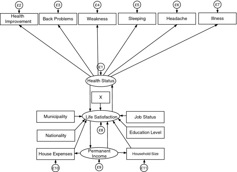
Figure 1. Path Diagram of the Effects on Life Satisfaction.
4. Data
The SHP started in 1999 with slightly more than 5000 households and it includes questions about the household composition and socioeconomic demographics. This study uses the SHP waves 2–15, that is, years 2000–2013.1 Based on the happiness literature (Clark and Oswald, 1994, 1996; Ferreira and Moro, 2010; Ferreira et al., 2013) the demographic and household variables of interest are household income, gender, age, household size, health status, job status, house tenure, marital status, education level, municipalities and community typology, such as whether the area is urban, sub-urban among others. In addition, the regressions consider the day of the week, the month of the year, the wave of the survey and area specific trends. The weather conditions are additionally considered, as they can influence life satisfaction and these are: the average temperature, the difference between the maximum and minimum temperature – which proxies for clear skies and humidity – (Levison, 2012), the precipitation and the wind speed. The dependent variable is the life satisfaction which is an ordered variable measured in a Likert scale from 0 (not satisfied at all) to 10 (completely satisfied).
In order to map and convert the point data from the monitoring stations into data up to zip code level we used the inverse distance weighting (IDW); a GIS-based interpolation method with a radius of 20 km including the 90% of the SHP sample. There are 2551 municipalities and the SHP is based on 2198 municipalities. Based on Table 1, the air pollutants present a significant deviation among them. For this reason the standardised coefficients are obtained.
Table 1. Summary Statistics.
| Air pollutant | Mean | Standard deviation | Min | Max |
| Life satisfaction | 8.027 | 1.467 | 0 | 10 |
| Equivalent household income | 56,670.47 | 57,456.89 | 0 | 5,541.319 |
| O3 | 56.6671 | 27.232 | 1.19 | 215.22 |
| SO2 | 2.531 | 1.992 | 0.12 | 60.14 |
| NO2 | 31.325 | 24.755 | 0.03 | 103.97 |
| CO | 381.761 | 343.385 | 0.0 | 1988.74 |
| PM10 | 20.903 | 12.005 | 0.70 | 195.14 |
Note: Air pollutants are measured in micrograms per cubic meter (μg/m3).
In Table 2, the correlation coefficients between the various pollutants and the life satisfaction are reported. These correlations are based on the average pollution levels at the nearest monitoring station at the day before the interview. The correlation between all air pollutants is positive with the exception of the ground-level ozone. The negative correlation between O3 and the other pollutants is induced by seasonal variations in the occurrence of these pollutants. More specifically, O3 is formed in high temperature and solar radiation levels, especially during summer (Bauer and Langmann, 2002; Toro et al., 2006). The remained pollutants are coming caused mainly from cars, trucks and buses, power plants, industry, landfills and not from weather; however their impact depends on the latter. More specifically, the main pollutants from diesel fuel vehicles include CO and NO2 from which the secondary pollutant O3 is formed (Charron and Harrison, 2003; Toro et al., 2006). The positive correlation between CO and NO2 is explained by the fact that the effect of CO is that it slowly burns nitrogen monoxide (NO) to NO2 (Vingarzan, 2004). Nitrogen oxides are mainly originated from anthropogenic sources and the increased production of O3 in the lower layer which the latter is associated with volatile organic compounds (VOCs), besides temperature and solar radiation (Wennberg et al., 1998; Bauer and Langmann, 2002; Toro et al., 2006). In other studies a positive correlation between CO, NO2 and SO2 has been found (Wang et al., 2002).
Table 2. Correlation between Air Pollutants and Life Satisfaction.
| Life satisfaction | O3 | SO2 | NO2 | CO | PM10 | |
| O3 | −0.0109*** | |||||
| (0.000) | ||||||
| SO2 | −0.0113*** | −0.1353*** | ||||
| (0.000) | (0.000) | |||||
| NO2 | −0.0098*** | −0.5078*** | 0.3078*** | |||
| (0.000) | (0.000) | (0.000) | ||||
| CO | −0.0057*** | −0.2620*** | 0.0788*** | 0.4680*** | ||
| (0.0000) | (0.0000) | (0.000) | (0.000) | |||
| PM10 | −0.0078*** | −0.4094*** | 0.2860*** | 0.7173*** | 0.3160*** | |
| (0.0000) | (0.0000) | (0.000) | (0.000) | (0.0002) | ||
| Household income | 0.0904*** | −0.0217*** | −0.0173*** | −0.0102*** | −0.0079** | −0.0084** |
| (0.0000) | (0.000) | (0.000) | (0.000) | (0.0138) | (0.0204) |
Note: p-Values are in brackets, *** and ** indicate significance at 1% and 5% level.
Based on the correlation matrix in Table 2, the association between household income and the air pollutants examined. Since the correlation does not give enough information for the relationship between income and air pollution the Environmental Kuznets Curve (EKC) hypothesis is examined and the results are presented in Figures 2–6 for linear and quadratic predicted values of the air pollutants. The EKC hypothesis has been inspired by Kuznets (1955) who predicted that the relationship between income inequality and per-capita income is characterised by an inverted U-shaped curve. This suggests that as the income is increased the income inequality initially is increased too, while the latter starts declining after a specific turning point of income. Following Kuznets (1955), EKC assumes the environmental degradation or pressure increases up to a certain level of income and after that it decreases implying that the environmental impact indicator is an inverted U-shaped function of income per capita. The majority of the studies exploited panel data based on country level and they found that the EKC hypothesis holds (Grossman and Krueger, 1993, 1995; Panayotou, 1997; Selden and Song, 1994; Vollebergh et al., 2009). In another study, Bölük and Mert (2014) examined the carbon dioxide emissions in 16 European Union (EU) countries by separating the final energy consumption into fossil fuel and renewable energy consumption. The authors found the EKC hypothesis does not hold and they suggest that a shift in renewable energy might decrease the greenhouse gas emission, because it contributes by around 50% less per unit energy that it is consumed by the conventional fossil energy use.
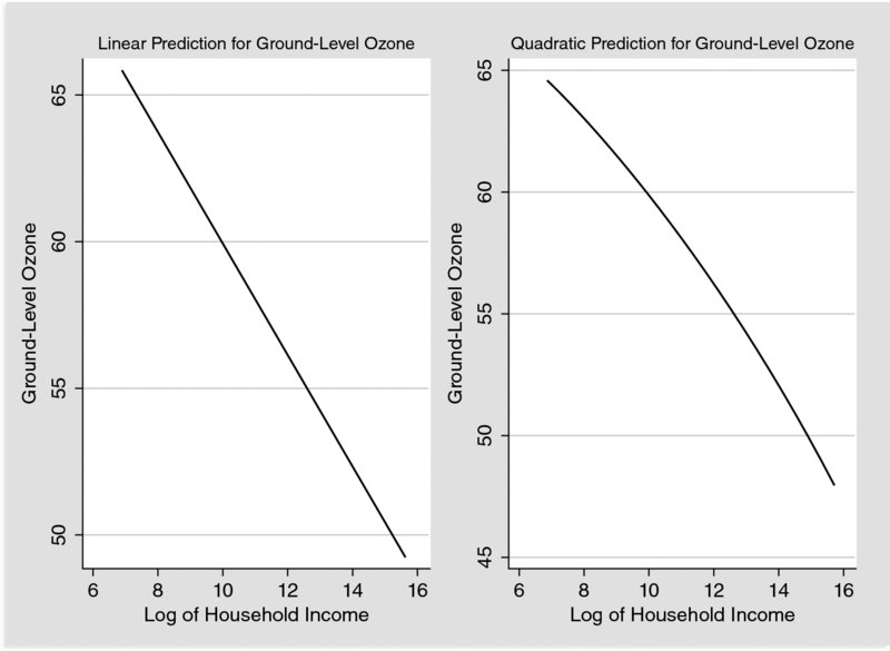
Figure 2. Linear and Quadratic Prediction Plots between Ground Level Ozone and Household Income.
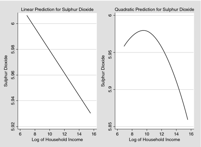
Figure 3. Linear and Quadratic Prediction Plots between Sulphur Dioxide and Household Income.

Figure 4. Linear and Quadratic Prediction Plots between Nitrogen Oxides and Household Income.

Figure 5. Linear and Quadratic Prediction Plots between Carbon Monoxide and Household Income.

Figure 6. Linear and Quadratic Prediction Plots between Particulate Matter and Household Income.
In Figures 2–6 the relationship between the air pollutants and the household income per capita considering linear and quadratic terms is presented. In all cases the cubic term on income is insignificant, as well as the EKC hypothesis and the shape holds either controlling or not for additional individual and household characteristics. According to the left side of the Figures 2–6 the relationship between income and the air pollutants is linear and negative, confirming so far the correlation in Table 2. Regarding the quadratic term on income is insignificant in the cases of O3 and CO presented in Figures 2 and 5. However, there is a significant relationship between the remained air pollutants and the income expressed in both linear and quadratic terms. Thus, the correlation standalone is not enough to reveal the relationship between income and pollution, where for SO2, NO2 and PM10 there is a quadratic relationship according to the figures on the right side suggesting that an inverted U-shaped curve exists for these pollutants and the EKC hypothesis holds. Previous studies suggest that the EKC hypothesis may be varied depending on various factors, such as the period examined, the type of the data analysis, which can be time-series, cross-sectional or panel data or it can be a matter of the specification from of the function estimated (Panayotou, 1997; Selden and Song, 1994; Vollebergh et al., 2009; Giovanis, 2012). Nevertheless, these issues are not the main interest of the study and overall the EKC hypothesis holds for SO2, PM10 and NO2 and the turning points are, respectively, $22,500 and $26,300 and $32,200. It should be noticed that the relationships do not change when the income expressed in levels instead in logarithms is considered.
5. Empirical Results
The results are reported in Table 3, while the findings for the socio-economic and personal characteristics are not explicitly discussed here as it is out of the study's scope. Overall, the findings are generally consistent with other studies (Luechinger, 2009; Levinson, 2012). Married are more satisfied than singles, while divorced and widowed are more likely to be less satisfied with their lives than singles are. Regarding job status, unemployed report lower levels of life satisfaction than those who are full time employed, while there is no difference between retired and part time employed. The home owners report higher levels of life satisfaction, while it seems that household size is associated negatively with life satisfaction. Finally, increases on average temperature and the difference between maximum and minimum temperature are associated with increases on life satisfaction. On the other hand, the relationship between life satisfaction and wind speed is negative, as higher wind speed is associated, with lower temperature. Even though wind speed can clean the air from pollutants the lower temperatures associated with it can have stronger effect on life satisfaction.
Table 3. Life Satisfaction Estimates for Nonmovers.
| Variables | Adapted Probit FE | SEM |
| Log of equivalent household income | 0.0774*** | 0.1015*** |
| (0.0138) | (0.0083) | |
| O3 | −0.0023*** | −0.0022*** |
| (0.0007) | (0.0002) | |
| SO2 | −0.0031*** | −0.0033*** |
| (0.0006) | (0.0007) | |
| NO2 | −0.0017*** | −0.0018*** |
| (0.0005) | (0.0004) | |
| CO | −0.0005** | −0.0006** |
| (0.0003) | (0.0003) | |
| PM10 | −0.0006** | −0.0007*** |
| (0.00033) | (0.0003) | |
| Average temperature | 0.0008*** | 0.0006*** |
| (0.0002) | (0.0003) | |
| Maximum–minimum temperature | 0.0003*** | 0.0004*** |
| (0.00013) | (0.0002) | |
| Wind speed | −0.0009*** | −0.0007*** |
| (0.0002) | (0.0002) | |
| Precipitation | 0.0003 | 0.0004 |
| (0.0002) | (0.0003) | |
| Age | −0.1709*** | −0.1425*** |
| (0.0066) | (0.0430) | |
| Age square | 0.0019*** | 0.0024*** |
| (0.0003) | (0.0008) | |
| Age cubic | −1.11e-0.5*** | −1.21e-0.5*** |
| (2.13e-06) | (4.76e-06) | |
| Household size | −0.0081* | −0.0126*** |
| (0.0042) | (0.0040) | |
| Job status (ref = full-time) | ||
| Job status (part-time) | −0.0113 | −0.0114 |
| (0.0202) | (0.0213) | |
| Job status (unemployed) | −0.3786*** | −0.3189*** |
| (0.0670) | (0.1163) | |
| Job status (retired) | −0.0326 | −0.0320 |
| (0.0369) | (0.0409) | |
| Marital status (ref = single) | ||
| Marital status (married) | 0.1321*** | 0.1624*** |
| (0.0353) | (0.0235) | |
| Marital status (widowed) | −0.2934*** | −0.3046** |
| (0.1050) | (0.1346) | |
| Marital status (divorced) | −0.2916* | −0.2640* |
| (0.1685) | (0.1710) | |
| Tenure (ref = tenant) | ||
| Tenure house (owner/co-owner) | 0.0491** | 0.0450*** |
| (0.0241) | (0.0091) | |
| Education (ref = incomplete compulsory school) | ||
| Education level (compulsory elementary school) | −0.0703*** | −0.0595** |
| (0.0196) | (0.0275) | |
| Education level (technical or vocational school) | 0.0399 | 0.0344 |
| (0.0556) | (0.0498) | |
| Education level (university) | −0.0598* | −0.0823*** |
| (0.0320) | (0.0282) |
| Variables | Adapted Probit FE |
SEM | t-Statistic for the difference of MWTP between FE and SEM (MWTPFE – MWTPSEM) |
| No. of obs. | 71,084 | 71,084 | |
| R2 | 0.3218 | ||
| AIC statistic | 89,896.56 | 81,992.01 | |
| BIC statistic | 90,863.73 | 82,341.65 | |
| χ2/df | 0.164 | ||
| Root mean square error of approximation (RMSEA) | 0.0025 | ||
| CFI | 0.945 | ||
| TLI | 0.924 | ||
| RMS | 0.010 | ||
| MWTP for a drop of one standard | $8,900 | $6,710 | 167.365 |
| deviation in O3 per year | [0.000] | ||
| 165.482 | |||
| MWTP for a drop of one standard | $11,995 | $9,876 | [0.000] |
| deviation in SO2 per year | 163.638 | ||
| MWTP for a drop of one standard | $6,580 | $5,390 | [0.000] |
| deviation in NO2 per year | 114.571 | ||
| MWTP for a drop of one standard | $1,940 | $1,680 | [0.000] |
| deviation in CO per year | 101.041 | ||
| MWTP for a drop of one standard deviation in PM10 per year | $2,320 | $2,135 | 0.000 |
Note: Standard errors are in brackets ***, ** and * indicate significance at 1%, 5% and 10% level. p-values are in square brackets.
The first remarkable finding is the cubic relationship between age and life satisfaction. While previous studies found that life satisfaction is rather flat throughout the life cycle (Myers, 2000) or there is an inverted U-shaped association (Easterlin, 2006), the findings in this study shows that after some point of the life cycle life satisfaction is reduced. The second remarkable finding is that there is a negative relationship between education level and life satisfaction, while a positive relationship is usually found (Easterlin, 2001, 2006; Bruni and Porta, 2005; Ferreira et al., 2013; Giovanis, 2014). On the other hand, these estimates are consistent with other studies which found a negative relationship especially in the developed nations (see e.g. Veenhoven, 1996; Dockery, 2003, 2010). This brings a great interest to further understand the relationship between education and subjective wellbeing. From previous research it is well established from both human capital theory and empirical evidence that higher educational attainment can enhance a person's future outcomes, including better career and employment opportunities increasing income and wealth and thus health outcomes (Sweetland, 1996). One possible explanation can be the fact that people who do well in education are those who tend to be happy and mentally resilient in the first place and that attaining educational qualifications per se makes little difference. Thus, education may have a negative impact, for example through raising aspirations and expectations that are not met and by leading to occupations that carry high levels of stress. More specifically, studies from Britain and the USA found a negative correlation between education and job satisfaction, indicating dissatisfaction among individuals with higher levels of education (Clark and Oswald, 1996; Ross and van Willigen, 1997; Stutzer, 2004; Verhaest and Omey, 2009). This dissatisfaction may be due to the lack of jobs at higher levels and the expectation of high educated individuals, the stress related to jobs at higher positions, and to mismatches between aspiration and expectations with employment possibilities for high educated people. Therefore, education can be significantly related to job satisfaction and as the latter is an important component of the life satisfaction, including income, health and other factors, leading to the negative relationship between higher educated people and their life satisfaction. Previous studies employing the Swiss Household Panel survey found the same concluding remarks (Stutzer, 2004; Krause, 2010). However, this needs further in-depth investigation as the relationship may vary depending on gender, age and health among other factors.
Regarding SEM, it is a useful tool which allows us to explore the direct and indirect effects. More specifically, as it has been shown in Figure 1 and the methodological framework, education has direct effects on life satisfaction and indirect effects through permanent income. Thus, the results show that while the indirect effects of education on life satisfaction through income are positive, the direct effects are negative. However, the total effects presented in Table 3 are negative as the direct effects exceed the indirect effects. These results can be explained as follows. Higher and better education provides individuals with better labour and market opportunities leading to increase on income, wealth and health outcome. This further leads to life satisfaction increase because income and wealth are tools which allow people to achieve specific goals and targets. On the other hand, education may present this direct negative association with life satisfaction, since individual have accomplished many goals regarding the educational attainment and achievement leaving them with less room for increases in life satisfaction relatively to people who still try to study, educate themselves and accomplish additional goals in their lives.
Based on Table 3 and the adapted Probit FE estimates, increasing O3, SO2, NO2, CO and PM10 by one standard deviation reduces life satisfaction by 0.0023, 0.0031, 0.0017, 0.0005 and 0.0006, respectively. The respective MWTP values expressed in 2013 US dollar prices are $8900, $11,995, $6580, $1940 and $2320. More specifically, based on the relation (2), the MWTP is the ratio of the partial derivative of life satisfaction with respect to air pollutant explored over the partial derivative of life satisfaction with respect to the logarithm of the household income. Then this ratio is multiplied by the average household income in order to calculate the MWTP in monetary values (Welsch, 2002, 2006; Luechinger, 2009; Levinson, 2012). The estimate air pollutant coefficients are small; however the results are consistent with the findings of previous studies. For instance Levinson (2012) found the estimated coefficients of the standardised PM10 and O3 equal at 0.0014 and 0.00021. The low estimated air pollutant coefficients may be due the air quality improvement during the period examined. Moreover, it might be the case that the public goods or the public bads in our case, play a lower or less significant role on overall well-being and life satisfaction than the personal and household characteristics do, such as income, employment status, marital status and others. In addition, when no controls are included into the regressions the air pollutant coefficients are larger, but controlling for additional individual and household characteristics their effect is reduced as expected, confirming the importance of other factors on life satisfaction. In addition, these controls may be correlated with air pollutants, like marital status, education and employment.
The results in Table 3 refer to MWTP for changes in standard deviation. More specifically, the MWTP for one standard deviation change in O3, which is equal at 27 and the average value of O3, which amounts to 56, constitutes a 48% change in O3. The percentage changes in the remained pollutants for one standard deviation change are: 78%, 76%, 90% and 60% for SO2, NO2, CO and PM10, respectively.
Regarding the SEM the results are reported in the second column of Table 3. In this case it is observed that the income effect on life satisfaction is higher than the respective one derived from the adapted Probit FE and it is equal at 0.1015. This has as a consequence that the MWTP will be lower and the values are: $6710, $9876, $5390, $1930 and $2135, respectively, for O3, SO2, NO2, CO and PM10. Thus, the MWTP derived by SEM are less by 15–25% for O3, SO2 and NO2, while the respective reduction for CO and PM10 ranges between 5% and 8%. In Table 3, the t-statistic and the respective p values for the comparison of the mean MWTP between adapted Probit FE and SEM are reported. In all cases it is concluded that the MWTP values are statistically different. The same concluding remarks are derived with the bootstrap t-statistics. The chi-square goodness-of-fit test and the root mean square error of approximation (RMSEA) descriptive model fit statistic are reported. The chi-square test of model fit is not significant and the RMSEA value 0.0025 is much lower than the value of 0.05 proposed by Hu and Bentler (1999) as an upper boundary. Moreover, the CFI and TLI are very close to unit and equal at 0.95 and 0.92, respectively, while RMSR 0.010, much lower than the proposed value of 0.1. Thus, based on these statistics it is concluded that the proposed model fits the data well.
In Table 4, the estimates of life satisfaction regressions for the movers sample are reported. While the household income is significant not all the air pollutants are. This can be explained by the fact the movers sample is endogenous and not stable across location and time. More specifically, there are individuals that have moved more than once across the period examined to areas with varying air pollution levels and types creating this bias in the estimates. In addition, it has been found that SO2 and O3 have strongest effect for non-movers than movers, as well as more persistent effects than the rest of the air pollutants. This can have various explanations. First, O3 has slightly been increased, while the other pollutants presented a significant declining and especially CO. Second, even if O3 and SO2 are invisible, they are mainly responsible for the formation of the winter smog (SO2) and for summer smog (O3), thus they can be observed and felt by people (Ponka, 1990; Medina-Ramon et al., 2006) Moreover, there is evidence that O3 produces short-term effects on mortality and respiratory morbidity, even at the low concentration levels (Ponka, 1990) while the effects of SO2 are direct, especially on health, and its effects are felt very quickly, where most people would feel the worst symptoms in 10–15 minutes after breathing. Furthermore, air pollutants have different effects on health and thus on peoples’ life satisfaction, since it is the most important component of the life satisfaction as it can be confirmed by the estimates in Table 3. For instance, a study in Helsinki, found that in a model containing temperature, NO, NO2, CO, SO2, O3 and PM10, simultaneously, NO, O3 and CO alone were significant predictors of respiratory hospital admissions (Ponka, 1990). On the other hand, SO2 and PM10 have been found to have more significant adverse effects on cardiovascular diseases than O3 (Ponka, 1990; Medina et al., 2006; Brauer et al., 2012). Schwartz (1991) analysed the relationship between air pollution and daily mortality in Detroit, during the period 1973–1982 and he found a positive relationship between mortality and particulate matters, but no significant relationship between mortality, O3 and SO2. Schwartz et al. (1991) explored the variation of the daily hospital admissions and the daily visits to paediatricians for obstructive bronchitis in children in five German towns in the mid-1980s and they found that in regression models where only one pollutant was included – SO2, NO2 and total suspended particles (TSP) – were all significant, where TSP is an archaic measure of PM which has been replaced afterwards. However, in the two pollutant models NO2 and SO2 were both insignificant, while TSP remained significant in the regression with SO2. A study exploring the long term effects of air pollution in a Dutch cohort, black smoke (BS) and nitrogen dioxide (NO2) were found to be positively associated with respiratory mortality but not significant estimates were found for SO2 and PM2.5 (Beelen et al., 2008) Therefore, the studies are mixed finding negative effects of every pollutant depending on the area and period examined. Moreover, the results of this study cannot be fully compared with previous studies, since it examines the five most important pollutants, while the previous studies explored a less number of air pollutants (Levinsion, 2012; Welsch, 2002, 2006).
Table 4. Life Satisfaction Estimates for Movers.
| Variables | Adapted Probit FE | SEM |
| Log of equivalent household income | 0.1201** | 0.1344** |
| (0.0526) | (0.0572) | |
| O3 | −0.0038 | −0.0045 |
| (0.0073) | (0.0051) | |
| SO2 | −0.0054 | −0.0057 |
| (0.0065) | (0.0041) | |
| NO2 | −0.0025** | −0.0032* |
| (0.0012) | (0.0017) | |
| CO | −0.0011 | −0.0014 |
| (0.0023) | (0.0012) | |
| PM10 | −0.0014* | −0.0018 |
| (0.0008) | (0.0014) | |
| No. of obs. | 3,517 | 3,517 |
| R2 | 0.4321 | |
| Root mean square error of approximation (RMSEA) | 0.0683 | |
| CFI | 0.883 | |
| TLI | 0.845 | |
| RMS | 0.084 | |
| MWTP for a drop of one standard deviation in O3 per year | ||
| MWTP for a drop of one standard deviation in SO2 per year | ||
| MWTP for a drop of one standard deviation in NO2 per year | $6,169 | $4,480 |
| MWTP for a drop of one standard deviation in CO per year | ||
| MWTP for a drop of one standard deviation in PM10 per year | $3,454 |
Note: Standard errors are in brackets, ** and * indicate significance at 5% and 10% level.
In Table 5, the robustness checks for the life satisfaction regressions and the non-movers sample are presented. More specifically, three alternative methods are applied, the OLS with fixed effects, the ‘BlowUp and Cluster’ (BUC) estimator (see Baetschmann et al., 2015 for technical details), and the GMM system (Blundell and Bond, 1998). The results are similar and the MWTP are close to those found with the Probit adapted fixed effects, with the exception of the GMM, whose MWTP are closer to those derived by the SEM relatively to the other methods. It should be noted that the estimated coefficients of BUC are higher than the coefficients obtained from the other methods, since BUC uses the binary conditional logit model and the coefficients are always higher than OLS regressions. Moreover, the number of observations is much less in BUC, which is common in the cases where variables are constant. More precisely, if an individual reports the same level of life satisfaction, that is, takes value 1 during the whole period examined, then it will be dropped from the sample. This can be one disadvantage of the BUC estimator, as also the estimates with fixed effects do not suffer when the well-being variable is measured in a wide scale from 0 to 10. On the other hand, the main issue is the possible degree of reverse causality between income and life satisfaction.
Table 5. Life Satisfaction Robustness checks for Nonmovers.
| Variables | OLS fixed effects |
GMM system |
BUC |
| Life satisfaction one lag | 0.1334*** | ||
| (0.0078) | |||
| Log of equivalent household income | 0.0687*** | 0.0954*** | 0.2143*** |
| (0.0315) | (0.0071) | (0.0713) | |
| O3 | −0.0025*** | −0.0024*** | −0.0081** |
| (0.0008) | (0.0005) | (0.0038) | |
| SO2 | −0.0033*** | −0.0030*** | −0.0108** |
| (0.0007) | (0.0004) | (0.0053) | |
| NO2 | −0.0016** | −0.0018*** | −0.0058* |
| (0.0007) | (0.0001) | (0.0023) | |
| CO | −0.0005* | −0.0007** | −0.0017** |
| (0.0003) | (0.0003) | (0.0018) | |
| PM10 | −0.0007* | −0.0008** | −0.0020* |
| (0.00038) | (0.0004) | (0.0025) | |
| No. of obs. | 71,084 | 55,892 | 58,419 |
| R2 | 0.3476 | ||
| Wald chi-square | 8913.30 | 9711.1 | |
| [0.000] | [0.000] | ||
| Arellano-Bond test for AR(2) in first differences | 1.65 | ||
| [0.208] | |||
| Exogeneity test | 0.40 | ||
| LR chi-square | [0.818] | ||
| MWTP for a drop of one standard deviation in O3 per year | $9,206 | $8,180 | $8,535 |
| MWTP for a drop of one standard deviation in SO2 per year | $12,935 | $11,175 | $11,320 |
| MWTP for a drop of one standard deviation in NO2 per year | $6,725 | $5,685 | $6,270 |
| MWTP for a drop of one standard deviation in CO per year | $2,135 | $1,905 | $1,935 |
| MWTP for a drop of one standard deviation in PM10 per year | $2,510 | $2,150 | $2,300 |
Note: Standard errors are in brackets, ***, ** and * indicate significance at 1%, 5% and 10% level. p-values are in square brackets.
Overall, all the studies examine the mean change and not standard deviation, with the exception the study by Levinson (2012). However, he examined the PM10 in the USA and the MWTP was found equal at $15,000 in 2012 prices, which is close to our findings, regarding SO2 and the fixed effects model. However, this study examines additional air pollutants, relies on more precise geographical and spatial area for the air mapping and uses actual income levels rather than mid-points of income scales as it is employed in the study by Levinson (2012).
However, one issue is that the air pollution depends on the location that respondents are moving to, which can be heterogeneous and since the air pollutants are significantly correlated as it has been seen in Table 2, the MWTP of one pollutant may partially represent the MWTP of another. For instance, the MWTP for O3 may partly represent the MWTP value for NO2. In order to explore the individual MWTP separate regressions for each pollutant are taken place for both mover and non-movers. In this case it could be argued that the omitted variable bias can be an issue since air pollutants are correlated, but it does not imply that are also confounders. The results are presented in Table 6, where only the coefficients of main interest are reported which are the air pollutants and the income. Based on the results the estimated coefficients for CO and O3 are insignificant in the movers sample, while the effects of PM10 and NO2 are found to be higher than the respective effects found in Table 3. and 4 Moreover, as it has been discussed in the methodology section, limiting the sample to non-movers may reduce the endogeneity issue coming from residential mobility; however it creates another selection bias due the fact that some of the respondents have already moved to cleaner or dirtier areas before the survey implementation. More specifically, this study proposes a Heckman Selection model into a Structural Equation Modelling framework. This is acceptable since the Heckman model is a two-step model. In particular, in the first step a binary Probit model is estimated exploring the determinants of the selection variable, where in the case examined is the moving status, and then the Inverse Mills ratio is calculated. In the second step the observation function is estimated, which is the life satisfaction, including the same factors as previously, where the Inverse Mills ratio is included as an additional regressor. In the case that Mill ratio is insignificant, it can be claimed that there is no selection bias. Furthermore, it should be noticed, that since panel data are employed, the first step includes a Logit rather than a Probit model, because the former allows for fixed effects. Therefore, the Heckman selection model is applied and the results are presented in Table 7. Finally, the annual averages of the air pollutants and the annual household income with one lag are considered. The reason for this specification is that we find to be more reasonable to explore the probability of the respondents having moved to another location given the pollution and household income one year before, since the survey is conducted annually.
Table 6. Life Satisfaction SEM Estimates for Air Pollutants.
| Variables | Panel A: Nonmovers | ||||
| Log of equivalent household | 0.1015*** | 0.1080*** | 0.1004*** | 0.1079*** | 0.1021*** |
| income | (0.0179) | (0.0198) | (0.0176) | (0.0198) | (0.0187) |
| O3 | −0.0022*** | ||||
| (0.0009) | |||||
| SO2 | −0.0036*** | ||||
| (0.0011) | |||||
| NO2 | −0.0019** | ||||
| (0.0008) | |||||
| CO | −0.0009** | ||||
| (0.0004) | |||||
| PM10 | −0.0017** | ||||
| (0.0008) | |||||
| No. of obs. | 71,172 | 71,128 | 71,225 | 71,112 | 71,121 |
| MWTP for a drop of one standard deviation in air pollutant | $6,200 | $10,100 | $5,500 | $2,500 | $5,100 |
| Panel B: Movers | |||||
| Equivalent household income | 0.1358** | 0.1353** | 0.1351* | 0.1338** | 0.1325** |
| (0.0618) | (0.0625) | (0.0622) | (0.0782) | (0.0582) | |
| O3 | −0.0020 | ||||
| (0.0014) | |||||
| SO2 | −0.0031* | ||||
| (0.0014) | |||||
| NO2 | −0.0029* | ||||
| (0.0015) | |||||
| CO | −0.0010 | ||||
| (0.0013) | |||||
| PM10 | −0.0019* | ||||
| (0.0007) | |||||
| No. of obs. | 3,526 | 3,522 | 3,532 | 3,525 | 3,523 |
| MWTP for a drop of one standard deviation in air pollutant | $4,700 | $8,300 | $4,300 | $2,200 | $5,000 |
Note: Standard errors are in brackets***, ** and * indicate significance at 1%, 5% and 10% level.
Table 7. SEM and Heckman Selection Model Fixed Effects.
| Variables | Observation equation DV: life satisfaction | |||||
| Log of equivalent household | 0.1029*** | 0.1040*** | 0.1016*** | 0.1050*** | 0.1006*** | |
| income | (0.0291) | (0.0272) | (0.0275) | (0.0281) | (0.0274) | |
| O3 | −0.0021** | |||||
| (0.0009) | ||||||
| SO2 | −0.0035** | |||||
| (0.0016) | ||||||
| NO2 | −0.0018* | |||||
| (0.0010) | ||||||
| CO | −0.0009* | |||||
| (0.0005) | ||||||
| PM10 | −0.0017** | |||||
| (0.0006) | ||||||
| Selection equation DV: moving status | ||||||
| Equivalent household income | −0.0411** | −0.0402** | −0.0397** | −0.0394** | −0.0396** | |
| (0.0182) | (0.0183) | (0.0182) | (0.0182) | (0.0182) | ||
| O3 | 0.0052*** | |||||
| (0.0006) | ||||||
| SO2 | 0.0096** | |||||
| (0.0045) | ||||||
| NO2 | 0.0016* | |||||
| (0.0009) | ||||||
| CO | 0.0001*** | |||||
| (0.00004) | ||||||
| PM10 | 0.0038*** | |||||
| (0.0011) | ||||||
| Inverse Mills ratio | −0.2197 | −0.5306 | −0.3827 | −1.3975 | −0.7667 | |
| (1.102) | (1.396) | (1.168) | (1.317) | (1.282) | ||
| No. of obs. | 55,054 | 54,717 | 55,223 | 53,984 | 53,494 | |
| Wald chi-square | 1804.45 | 1768.01 | 1793.46 | 1434.71 | 1659.83 | |
| [0.000] | [0.000] | [0.000] | [0.000] | [0.000] | ||
| Rho | −0.2442 | −0.5337 | −0.4064 | −0.9127 | −0.6869 | |
| [0.842] | [0.704] | [0.743] | [0.289] | [0.650] | ||
| MWTP for a drop of one standard deviation in air pollutant | $6,100 | $10,000 | $5,400 | $2,600 | $5,100 | |
Note: Standard errors are in brackets, p-values within square brackets ***, ** and * indicate significance at 1%, 5% and 10% level.
Based on the results of Table 7 the probability of moving is the highest in the case of SO2 followed by O3 and PM10, while the respective probabilities are significantly lower in the cases of NO2 and CO. The MWTP for the air pollutants differ from the respective values found in Table 3 and are closer to SEM. However, the MWTP for PM10 and NO2 are higher and for O3 become lower. This might indicate that in Table 3 the estimates provide partially the MWTP for each pollutant, while in Table 4 and the movers sample most of the air pollutants are even insignificant. There is no clear explanation for these findings. One reason can be the fact that O3 is correlated with these two air pollutants, as well as, its formation depends on NO2 levels, besides the temperature and solar radiation. The small number of moving cases as the location they moved may be another cause. Another possible explanation is that conditioning on one or more variables the causal path is blocked-off. For instance, the effect of O3 on life satisfaction, when the regression is conditioning or controlling for PM10, might be blocked-off, for example, O3→PM10→LS and there is no indirect effect from O3 to life satisfaction (Spirtes et al., 2000; Pearl, 2000, 2009). Moreover, the inverse Mills ratio is insignificant in all cases indicating that there is no evidence that the selection bias is quantitatively important. Overall, the procedures in Tables 6 and 7. suggest that in order to consider in the analysis latent variables, accounting for measurement error and selection bias and to properly estimate the MWTP individually for each air pollutant the Heckman selection model into a Structural Equation Model framework can be an alternative valuable option.
The SEM estimates differ from the fixed effects from various aspects. First, it allows to treat health status and permanent income as latent variables accounting for measurement error. Even if the argument that income and expenditures can be a good measure of standard of living and well-being, they might be measured with error. Second, SEM allows a simultaneity regression approach accounting also for possible reciprocal effects between income and life satisfaction and between life satisfaction and health status. A simultaneous approach can be applied for example with seemingly unrelated regressions (SURE), but they do not treat the variables of interest as latent. Third, depending on the theoretical model examined it is possible to derive the direct and indirect effects of the explanatory variables. For instance, education has an indirect effect on life satisfaction as it acts as a causal indicator of permanent income and at the same time has a direct effect on life satisfaction. Similarly, the reciprocal effects between life satisfaction and health status can be explored as well as the indirect effects of health status on permanent income through life satisfaction. For instance based on Figure 1, job status has a direct effect on life satisfaction as well as an indirect effect through permanent income. The direct effect for an unemployed is –0.2505, while the indirect effect through income is –0.0684 resulting to a total effect of –0.3189. Additional relationships can be derived from Figure 1. Continuing with the unemployed, as the job status is a causal indicator of income, it has a direct effect on income equal at –0.1034 as it is expected since unemployed reduces the income. Additionally, there is an indirect effect through life satisfaction, since the model allows for reciprocal effect, and the effect is negative and equal at –0.0342 resulting to a total effect of –0.1376. Thus, unemployment can have a direct effect on income but also a moderating effect through life satisfaction, since less happy or satisfied people are more likely to earn less. Finally, the results support that there is a reverse causality as the people who report higher life satisfaction levels are associated with increases on income by 137.00 (SE: 10.480) Swiss franc on average, while the health is improved by 0.103 (SE: 0.0439). The estimated coefficients are not reported, but are significant at 1% and 5%, respectively. Similarly, other effects can be derived.
It should be noticed that SEM could include additional factors for the measurement equation of life satisfaction. More precisely, these are the emotion variables and their frequency, such as joy, worry, anger and sadness measured in the same scale as life satisfaction, from no frequency (taking value 0) to very frequent (taking value 10). The results are not presented here as the concluding remarks are the same and the coefficients sign is the same (i.e. positive effect of income and negative effect of air pollution on life satisfaction); however, are not the same. Regarding the emotion variables, a negative relationship between the frequency of anger, worry and sadness with life satisfaction is presented, while a positive association between joy and life satisfaction is reported. Moreover, the big five personality traits have been included into SHP in 2009 (wave 11) until 2011 (wave 13) which can be included in a similar fashion with the emotion variables. In this case the life satisfaction can be treated as a latent and unobserved variable and the SEM application could valuable since there might be measurement error in life satisfaction. However, this will restrict the sample of the analysis to 6 waves (and three waves for the personality traits) instead of 14 waves that have been used in this study. This is important because it is desirable, using panel data, to follow the same individual and examine the effects of air pollution across a long time of period. Nevertheless, this is proposed for further research including these factors as additional variables into the measurement equation of life satisfaction, as it has been described in the methodology part, as well as additional covariates in the life satisfaction regressions. Furthermore, using SEM framework, many effects through various paths can be additionally explored. More precisely the theoretical model in this study assumes a direct effect of air pollution on life satisfaction. However, it is likely that indirect effects through health status or job status might be evident, as air pollution affects the health which is a major element of the human capital and development and the impact on job status can be associated with productivity effect from air quality.
Overall, the findings suggest that the MWTP for the air pollutants examined, with the exception of SO2 and O3 are relatively low, since are measured in terms of standard deviation, reflecting probably the reduction followed in these air pollutants since 1990s (European Environmental Agency, 2013). It is suggested that the air quality has been improved in Switzerland and in 2010 the emissions overall were significantly lower than in 2000. However, in some (urban) areas, the combination of reduced NOx and an increasing contribution of hemispheric background ozone is leading to increasing ozone levels in cities and increased population exposures to ground-level ozone (European Environmental Agency, 2013). Moreover, ozone depends mainly on solar radiation and temperature and thus the peak levels are higher reach during the summer. Therefore, while there has been an improvement on air quality regarding the remained air pollutants examined in this study, O3 still has persistent effects owned also to climate change and increase on temperature. Regarding the high MWTP values for SO2 and O3 can also be explained that are observed by the people, as the former is responsible for the formation of winter smogs, while the latter is mainly responsible for the summer smogs. Since people are educated about the cause and effects of air pollutants, it is reasonable that the MWTP to be higher for these two air pollutants (Notholt et al., 2005). In Figures 7–11, the annual averages based on municipality level for the air pollutants during the period examined are reported. It becomes clear that there is a reduction for all pollutants, especially for CO. The only exception is O3 which presents a small increase. This can explain also the high MWTP for this pollutant.

Figure 7. Annual Ozone Averages by Municipality.

Figure 8. Annual Sulphur Dioxide Averages by Municipality.

Figure 9. Annual Nitrogen Dioxide Averages by Municipality.

Figure 10. Annual Carbon Monoxide Averages by Municipality.

Figure 11. Annual Particulate Matter less than 10 Microns Averages by Municipality.
6. Conclusions
The findings show that income effects are underestimated when the reverse causality is not considered leading to higher monetary values. In addition, the importance of this study comes from the fact that the analysis relies on detailed micro-level data, using highly spatially disaggregated data based on municipality zip codes, capturing more precise the air pollution effects, which are not captured in previous studies. Overall the results show that the MWTP are relatively low for NO2, CO and PM10, while the highest values are observed for O3 and SO2.
One important point revealed by this study, consistent with the previous researches is the negative and significant direct effects of air pollution on individuals’ well-being. Additionally, this study showed that there is evidence of a substantial trade-off between income and air quality. Larger scale researches, using more than one country and based on high spatially disaggregated data is suggested in order to clarify the potentially complex links between well-being, income and individuals’ exposure to air pollution. This could offer further insights to policy makers in order to achieve happier, cleaner and more sustainable cities. In addition, the life satisfaction approach as well as the SEM framework proposed can be useful for policy makers on environmental regulation decision making. Moreover, future structural modelling applications including additional robustness checks for gender, age groups, urban versus rural areas among others, is suggested. Furthermore, the application and test of SEM in other surveys and datasets, and the quest for the causal effects of income and public goods on life satisfaction can be continued.
Acknowledgements
The authors would like to thank the anonymous reviewers for their valuable comments, suggestions and constructive comments that greatly contributed to the improvement of the quality of this paper. Any remaining errors or omissions remain the responsibility of the authors.
The authors would also like to thank Denise Bloch at FORS, Bureau 5614 Quartier UNIL-Mouline Bâtiment Géopolis 1015 Lausanne for providing the access to the Swiss Household Panel Survey Data. In addition, they are grateful to Dr. Rudolf Weber at Eidg. Departement für Umwelt, Verkehr, Energie und Kommunikation UVEK Bundesamt für Umwelt BAFU Abteilung Luftreinhaltung und Chemikalien CH-3003 Bern, who provided the relevant air pollution data.
Note
References
- Adamowicz, W., Louviere, J. and Swait, J. (1998) Introduction to attribute-based stated choice methods. Final Report to National Oceanic and Atmospheric Administration (NOAA), US.
- Baetschmann, G., Staub, K.E. and Winkelmann, R. (2015) Consistent estimation of the fixed effects ordered Logit model. Journal of the Royal Statistical Society: Series A (Statistics in Society 178(3): 685–703.
- Bauer, S.E. and Langmann, B. (2002) Analysis of a summer smog episode in the Berlin-Brandenburg region with a nested atmosphere—chemistry model. Atmospheric Chemistry and Physics 2(4): 259–270.
- Bayer, P. and Timmins, C. (2005) On the equilibrium properties of locational sorting models. Journal of Urban Economics 57(3): 462–477.
- Bayer, P. and Timmins, C. (2007) Estimating equilibrium models of sorting across locations. Economic Journal 117(518): 353–374.
- Bayer, P., Keohane, N.O. and Timmins, C. (2009) Migration and hedonic valuation: The case of air quality. Journal of Environmental Economics and Management 58: 1–14.
- Beelen, R., Hoek, G., van den Brandt, P.A., Goldbohm, R.A. Fischer, P., Schouten, L.J., Jerrett, M., Hughes, E., Armstrong, B. and Brunekreef, B. (2008) Long-term effects of traffic-related air pollution on mortality in a Dutch cohort (NLCS-AIR Study). Environmental Health Perspectives 116(2): 196–202.
- Bentler, P.M. (1990) Comparative Fit Indexes in Structural Models. Psychological Bulletin 107(2): 238–246.
- Blundell, R. and Bond, S. (1998) Initial conditions and moment restrictions in dynamic panel data models. Journal of Econometrics 87: 115–143.
- Bollen, K.A. (1989) Structural Equations with Latent Variables. 1st edition, John Wiley & Sons, New York.
- Bölük, G. and Mert, M. (2014) Fossil and renewable energy consumption, GHGs (greenhouse gases) and economic growth: Evidence from a panel of EU (European Union) countries. Energy 74(1): 439–446.
- Brauer, M., Amann, M., Burnett, R.T., Cohen, A., Dentener, F., Ezzati, M., Henderson, S.B., Krzyzanowski, M., Martin, R.V., Van Dingenen, R., van Donkelaar, A. and Thurston, G. (2012) Exposure assessment for estimation of the global burden of disease attributable to outdoor air pollution. Environmental Science and Technology 46: 652–660.
- Bruni, L. and Porta, P. (2005) Economics and Happiness: Framing the Analysis. New York: Oxford University Press.
- Calabrese, S., Epple, S. and Romano, R. (2007) On the political economy of zoning. Journal of Public Economics 91(1–2): 25–49.
- Campbell, D. (2007) Willingness to pay for rural landscape improvements: Combining mixed Logit and random-effects models. Journal of Agricultural Economics 58(3): 467–483.
- Campbell, D., Hutchinson, G. and Scarpa, R. (2008) Incorporating discontinuous preferences into the analysis of discrete choice experiments. Environmental and Resource Economics 41: 401–417.
- Campbell, D., Hensher, D.A. and Scarpa, R. (2011) Nonattendance to attributes in environmental choice analysis: A latent class specification. Journal of Environmental Planning and Management 54(8): 1061–1076.
- Carson, R.T., Mitchell, R.C., Hanemann, W.M., Kopp, R.J., Presser, S. and Ruud, P.A. (2003) Contingent valuation and lost passive use: Damages from the Exxon Valdez oil spill. Environmental and Resource Economics 25: 257–286.
- Charron, A. and Harrison, R.M. (2003) Primary particle formation from vehicle emissions during exhaust dilution in the roadside atmosphere. Atmospheric Environment 37(29): 4109–4119.
- Clark, A.E. and Oswald, A.J. (1994) Unhappiness and unemployment. The Economic Journal 104: 648–659.
- Clark, A.E. and Oswald, A.J. (1996) Satisfaction and comparison income. Journal of Public Economics 61: 359–381.
- Croper, M.L. and Oates, W.E. (1992) Environmental economics: A survey. Journal of Economic Literature 302: 675–740.
- Dockery, A.M. (2003) Happiness, life satisfaction and the role of work: Evidence from two Australian surveys. HILDA Working Paper No.3/10.
- Dockery, A.M. (2010) ‘Education and happiness in the school-to-work transition’, National Centre for Vocational Education Research (NCVER), Adelaide.
- Easterlin, R. (2001) Income and happiness: Towards a unified theory. Economic Journal 111: 465–484.
- Easterlin, R.A. (2006) Life cycle happiness and its sources: Intersections of psychology, economics, and demography. Journal of Economic Psychology 27: 463–482.
- European Environmental Agency. (2013) Air Pollution Fact Sheet 2013 Switzerland. Copenhagen, Denmark: European Environment Agency.
- Ferreira, S. and Moro, M. (2010) On the use of subjective well-being data for environmental valuation. Environmental and Resource Economics 46(3): 249–273.
- Ferreira, S., Akay, A., Brereton, F., Cuñado, J., Martinsson, P., Moro, M. and Ningal, T.F. (2013) Life satisfaction and air quality in Europe. Ecological Economics 8: 1–10.
- Ferreyra, M.M. (2007) Estimating the effects of private school vouchers in multidistrict economies. American Economic Review 97(3): 789–817.
- Frey, B., Luechinger, S. and Stutzer, A. (2010) The life satisfaction approach to environmental valuation. Annual Review of Resource Economics 2: 139–160.
- Friedman, M. (1957) A theory of the consumption function. Princeton, New Jersey, USA: Princeton University Press.
- Giovanis, E. (2012) Environmental Kuznets curve: Evidence from the British household panel survey. Journal of Economic Modelling 30: 602–611.
- Giovanis, E. (2014) relationship between well-being and recycling rates: Evidence from life satisfaction approach in Britain. Journal of Environmental Economics and Policy 3(2): 201–214.
- Grossman, G.M. and Krueger, A.B. (1993) Pollution and growth: What do we know? In I. Goldin and L. Winters (eds.), The Economics of Sustainable Development. Cambridge, MA: MIT Press.
- Grossman, G.M. and Krueger, A.B. (1995) Economic growth and the environment. Quarterly Journal of Economics 110(2): 353–377.
- Hall, J.V., Winer, A.M., Kleinman, M.T., Lurmann, F.W., Brajer, V. and Colome, S.D. (1992) Valuing the health benefits of cleaner air. Science 255: 812–817.
- Hammitt, J.K. and Zhou, Y. (2006) The economic value of air-pollution-related health risks in China: A contingent valuation study. Environmental and Resource Economics 33: 399–423.
- Hancock, G. R. and Mueller, R. O. (2006) Structural equation modeling: A second course. Information Age Publishing, Inc. Greenwich, Charlotte, North Carolina, USA.
- Hanley, N., Koop, G., Wright, R. and Alvarez-Farizo, B. (2001a) Go climb a mountain: An application of recreational demand models to rock climbing. Journal of Agricultural Economics 52(1): 36–51.
- Hanley, N., Mourato, S. and Wright, R.E. (2001b) Choice modelling approaches: A superior alternative for environmental valuation? Journal of Economic Surveys 15(3): 435–462.
- Hauser, R.M. and Warren, J.R. (1997) Socioeconomic indexes for occupations: A review, update, and critique. In A.E. Raftery (ed.), Sociological Methodology (pp. 177–298). Cambridge: Blackwell.
- Heckman, J. (1979) Sample selection bias as a specification error. Econometrica 47(1): 153–161.
- Hernan, M.A., Hernandez-Diaz, S. and Robins, J.M. (2004) A structural approach to selection bias. Epidemiology 15: 615–625.
- Houthakker, H.S. (1957) The permanent income hypothesis: A review article. American Economic Review 47(2): 396–404.
- Hu, L. and Bentler, P.M. (1999) Cutoff criteria in fix indexes in covariance structure analysis: Conventional criteria versus new alternatives. Structural Equation Modeling 6(1): 1–55.
- Ioannides, Y.M. and Zabel, J.E. (2008) Interactions, neighbourhood selection and housing demand. Journal of Urban Economics 63: 229–252.
- Kahneman, D., Ritov, I. and Schkade, D. (1999) Economic preferences or attitude expressions? An analysis of dollar responses to public issues. Journal of Risk and Uncertainty 19: 220–242.
- Krause, A. (2010) The effect of unemployment on life and satisfaction an analysis for Switzerland in its cultural diversity. Working Paper, Lausanne. Available at: http://www.iza.org/conference_files/ReDisWeBe2010/krause_a5647.pdf (Retrieved on 15 August 2015)
- Kuminoff, N.V., Parmeter, C.F. and Pope, J.C. (2010) Which hedonic models can we trust to recover the marginal willingness to pay for environmental amenities? Journal of Environmental Economics and Management 63: 145–160.
- Kuminoff, N.V., Smith, V.K. and Timmins, C. (2013) The new economics of equilibrium sorting and policy evaluation using housing markets. Journal of Economic Literature 51(4): 1007–1062.
- Kuznets, S. (1955) Economic growth and income inequality. American Economic Review 45: 1–28.
- Levinson, A. (2012) Valuing public goods using happiness data: The case of air quality. Journal of Public Economics 96 (9–10): 869–880.
- Loehman, E. and De, V. (1982) Application of stochastic choice modeling to policy analysis of public goods: A case study of air quality improvements. The Review of Economics and Statistics 64: 474–480.
- Luechinger, S. (2009) Valuing air quality using the life satisfaction approach. Economic Journal 119(536): 482–515.
- Luechinger, S. (2010) Life satisfaction and transboundary air pollution. Economics Letters 1071: 4–6.
- MacKerron, G. and Mourato, S. (2009) Life satisfaction and air quality in London. Ecological Economics 685: 1441–1453.
- Mayer, T. (1963) The permanent income theory and occupational groups. Review of Economics and Statistics 45(1): 16–22.
- Medina-Ramon, M., Zanobetti, A. and Schwartz, J. (2006) The effect of ozone and PM10 on hospital admissions for pneumonia and chronic obstructive pulmonary disease: A National Multicity Study. American Journal of Epidemiology 163(6): 579–588.
- Muthen, B. and Asparouhov, T. (2012) Bayesian structural equation modeling: A more flexible representation of substantive theory. Psychological Methods 17(3): 313–335.
- Myers, D.G. (2000) The funds, friends, and faith of happy people. American Psychologist 55 (1): 56–67.
- Notholt, J., Luo, B.P., Fueglistaler, S., Weisenstein, D., Rex, M., Lawrence, M.G., Bingemer, H., Wohltmann, I., Corti, T., Warneke, T., von Kuhlmann, R. and Peter, T. (2005) Influence of tropospheric SO2 emissions on particle formation and the stratospheric humidity. Geophysical Research Letters 32: L07810, doi:10.1029/2004GL022159.
- Panayotou, T. (1997) Environmental Kuznets curve. Environment and Development Economics 2: 465–484.
- Pearl, J. (2000) Causality. Models, Reasoning, and Inference. Cambridge: Cambridge University Press.
- Pearl, J. (2009) Causal inference in statistics: An overview. Statistical Surveys 3: 96–146.
- Ponka, A. (1990) Absenteeism and respiratory disease among children and adults in Helsinki in relation to low level air pollution in Helsinki. Environmental Research 52: 34–46.
- Powdthavee, N. (2010) How much does money really matter? Estimating the causal effects of income on happiness. Empirical Economics 39: 77–92.
- Powdthavee, N. and Wooden, M. (2015) Life satisfaction and sexual minorities: Evidence from Australia and the United Kingdom. Journal of Economic Behavior and Organization 116: 107–126.
- Rabin, M. (1998) Psychology and economics. Journal of Economic Literature 361: 11–46.
- Rehdanz, K. and Maddison, D. (2008) Local environmental quality and life-satisfaction in Germany. Ecological Economics 64: 787–797.
- Ridker, R.G. and Henning, J.A. (1967) The determinants of residential property values with special reference to air pollution. The Review of Economics and Statistics 492: 246–257.
- Rosen, S. (1974). Hedonic prices and implicit markets: Product differentiation in pure competition. Journal of Political Economy 82: 34–55.
- Ross, C.E. and Van Willigen, M. (1997) Education and the subjective quality of life. Journal of Health and Social Behavior 38(3): 275–297.
- Scheines, R., Hoijtink, H. and Boomsma, A. (1999) Bayesian estimation and testing of structural equation models. Psychometrika 64: 37–52.
- Schwartz, J. (1991) Particulate air pollution and daily mortality in Detroit. Environmental Research 56: 204–213.
- Schwartz, J., Spix, C., Wichmann, H.E. and Malin, E. (1991) Air pollution and acute respiratory illness in five German communities. Environmental Research 56: 1–14.
- Selden, T. and Song, D. (1994) Environmental quality and development: Is there a Kuznets curve for air pollution emissions? Journal of Environmental Economics and Management 27: 147–162.
- Smith, V.K. and Huang, J.C. (1995) Can markets value air quality? A meta-analysis of hedonic property value models. Journal of Political Economy 1031: 209–227.
- Spirtes, P., Glymour, C. and Scheines, R. (2000) Causation, Prediction, and Search (2nd edn). Cambridge, MA: MIT Press.
- Stutzer, A. (2004) The role of income aspirations in individual happiness. Journal of Economic Behaviour and Organisation 54: 89–109.
- Stutzer, A. and Frey, B. (2012) Recent developments in the economics of happiness: A selective overview, Discussion Paper No 7978, The Institute for the Study of Labour (IZA), Bonn.
- Sweetland, S.R. (1996) Human capital theory: Foundations of a field of inquiry. Review of Educational Research 66(3): 341–359.
- Toro, M.V., Cremades, L.V. and Calbo, J. (2006) Relationship between VOC and NOx emissions and chemical production of tropospheric ozone in the Aburra Valley (Colombia). Chemosphere 65(5): 881–888.
- Tsui, H.C. (2014) What affects happiness: Absolute income, relative income or expected income. Journal of Policy Modeling 36(6): 994–1007.
- Tucker, L.R. and Lewis, C. (1973) A reliability coefficient for maximum likelihood factor analysis. Psychometrica 38(1): 1–10.
- Van Praag, B.M.S. and Ferrer-i-Carbonell, A. (2004) Happiness Quantified: A Satisfaction Calculus Approach. Oxford: Oxford University Press.
- Veenhoven, R. (1996) Developments in satisfaction research. Social Indicators Research 37: 1–46.
- Verhaest, D. and Omey, E. (2009) Objective over-education and worker well-being: A shadow price approach. Journal of Economic Psychology 30: 469–481.
- Vingarzan, R. (2004) A review of surface ozone background levels and trends. Atmospheric Environment 38(21): 3431–3442.
- Vollebergh, R.J.H., Melenberg, B. and Dijkgraaf, E. (2009) Identifying reduced-form relations with panel data: The case of pollution and income. Journal of Environmental Economics and Management 58(1): 27–42.
- Wang, T., Cheung, T.F. and Li, Y.S. (2002) Emission characteristics of CO, NOx, SO2 and indications of biomass burning observed at a rural site in eastern China. Journal of Geophysical Research 107(D12): 4157, doi:10.1029/2001JD000724.
- Welsch, H. (2002) Preferences over prosperity and pollution: Environmental valuation based on happiness surveys. Kyklos 55(4): 473–494.
- Welsch, H. (2006) Environment and happiness: Valuation of air pollution using life satisfaction data. Ecological Economic 58: 801–813.
- Wennberg, P.O., Hanisco, T.F., Jaegle, L., Jacob, D.J., Hintsa, E.J., Lanzendorf, E.J., Anderson, J.G., Gao, R.-S. Keim, E.R., Donnelly, S.G., Del Negro, L.A., Fahey, D.W., McKeen, S.A., Salawitch, R.J., Webster, C.R., May, R.D., Herman, R.L., Proffitt, M.H., Margitan, J.J., Atlas, E.L., Schauffler, S.M., Flocke, F., McElroy, C.T. and Bui, T.P. (1998) Hydrogen radicals, nitrogen radicals, and the production of O3 in the upper troposphere. Science 279(5347): 49–53.