
CHAPTER 5
Case Studies in Valuation During the Recent Decade
At the end of Chapter 4, we demonstrated a practical application of the valuation model. We did so under practice field conditions, meaning that we applied the model to clean data under controlled conditions. The next logical step is applying the model under competitive match conditions; doing this often means dirty or unusual data, time pressure, and other extraneous factors.
Consequently, in this chapter, we examine four companies over the past decade, 1995 to 2005, with a view toward understanding the complexities that arise under real-life conditions. The purpose is to demonstrate both strengths and weaknesses in our analytical construct.
As a matter of course, any sufficiently powerful model must rely on a high degree of abstraction and idealized representation. In a profound sense, this strength also embodies the fundamental weakness, that is, the problematic application in certain stress or unusual cases. We have therefore selected companies both to demonstrate the general resilience of the model and to propose certain commonsense adjustments for atypical or ill-behaved cases.
At the end of the day, we are well advised to keep in mind our goal of being “approximately right” rather than “precisely wrong.” Thus, we will not be excessively discouraged where we occasionally and inevitably find instances that prove intractable. While we could presumably simply create additional explanatory aspects of the model to turn the intractable into the manageable, our overall approach is to resist this temptation. I am firmly convinced through my years as a practitioner that, as many before have said, “The model that explains everything predicts nothing.”
The companies selected are The Coca-Cola Company (Coke), Intel Corporation, The Procter & Gamble Company (P&G), and Enron Corp. All are well-known names for which data are readily accessible. In addition, the companies are among those for which I have acquired a more than passing degree of familiarity in my career in investment portfolio management during the period under examination.
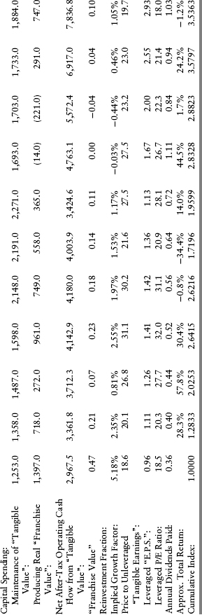
Table 5.1 summarizes key characteristics of all four companies, the first three for their 10 fiscal years ended 2005. The fourth company, Enron, did not survive intact for that entire period. For reasons that will become obvious, we elected to break the analytical period into two segments.
TABLE 5.1 Summary Statistics for Four Case Study Companies
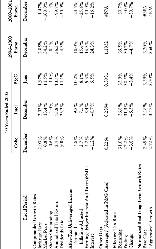
We will treat each of the companies in detail, but first we note a few points in the table. The period under examination was reflective of cumulative economic growth in line with the 3%+ inflation-adjusted gross domestic product (GDP) growth rate of U.S. history. In addition, inflation was neither particularly high nor variable during this 10-year period. There were the usual number of crises and complications: for example, Russian default crisis and Long Term Capital Management collapse and crisis in 1998, the September 11, 2001, terrorist attacks and related market disruptions, mass airline bankruptcies, overseas wars in Afghanistan and Iraq, the tech market bubble and ensuing collapse, and energy supply shocks. In sum, it was a fairly typical slice of economic and market history for the United States.
Taking a quick peek at the market price growth and total return numbers, Coke was a pronounced underperformer, while Intel and P&G both had very good returns. (As a reference point, the Standard & Poor’s (S&P) 500 Index posted a cumulative annualized total return of 9.1% per annum for the 10 calendar years ended 2005, 9.3% for the 10 fiscal years ended June 2005, and 18.3% for the 5 years ended December 2000.) Enron soared like Icarus prior to 2000 and subsequently suffered the same kind of ignominious crash.
Table 5.1 shows that Coke experienced a slower growth in earnings and cash flow, as compared with the more successful Intel and Procter & Gamble during the 10 years studied. It is easy to suppose that Coke was subject to a lower organic sales growth due to its products being largely consumer nondurables and due to stiffer competition from a renewed focus on “healthier” alternatives. However, in more objective terms, the core growth rate of 2.7% per year (after inflation) was nothing to be ashamed of. In fact, the average ratio of franchise-value-capital-spending to after-tax cash flow from operations was .2266 during the period. Combined with an assumed 11% inflation-adjusted return on equity (ROE; or z), this produces a sustainable growth rate of 2.49%.1
Given that the effective income tax rate fell noticeably over the decade, it is not surprising that the actual growth rate was modestly in excess of the core growth rates that are displayed at the bottom of the table.
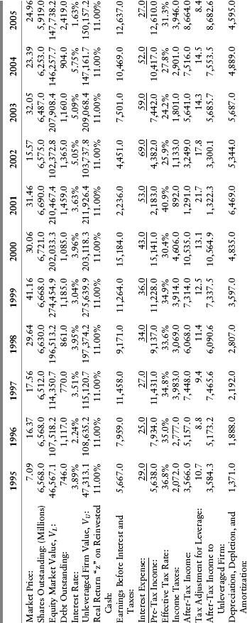
The necessary explanation must address why the cumulative market return was anemic despite reasonable long-term core growth. Rather than hastening to the answer, we need to take the time to investigate the puzzle one step at a time. We begin by presenting “broad-brush” year-by-year financial and operational fundamentals in Table 5.2.
TABLE 5.2 Coca-Cola Year-by-Year Analysis (amounts in $Millions, except per share amounts)
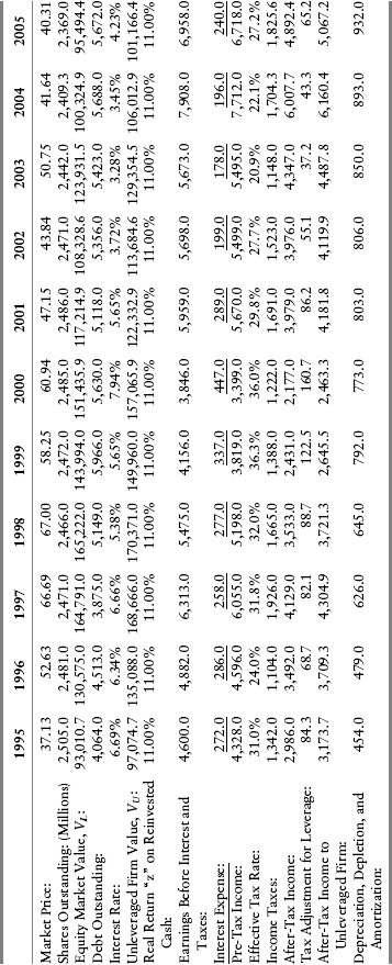
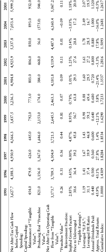
The historical information in this table and in the tables for our other company case studies was obtained primarily from 10-K filings provided to the Securities and Exchange Commission. Price and dividend information was obtained from the Wall Street Journal or from Fidelity Investments. Other estimates and mathematical formulations are the responsibility of the author.
One of the first things worth noting is that the ratio of (a) franchise-value-capital-spending to (b) net after-tax cash flow from operations varies considerably from year to year. This pattern is typical of most companies, both those discussed in this book and those in the marketplace. Capital spending for growth (or franchise value) opportunities is likely to be lumpy over time for one or more reasons:
1. Capital spending is likely to be more pronounced during periods of product market growth and business cycle optimism and less pronounced when such conditions are reversed.
2. Many capital-spending opportunities, such as new factories or substantial plant modifications, are few and far between, but are large relative to current year cash flow when they do occur.
3. Certain growth opportunities come in the form of purchases of entire companies or divisions. However, these arise only on an occasional and opportunistic basis.
With this observed variability in year-to-year investment ratios, Table 5.2 shows that there is quite a divergence between growth rates computed from such individual-year investment ratios and a long-term average ratio.
Our practitioner’s approach is therefore often to utilize an investment ratio f that reflects a full multiple-year capital-spending cycle. In Table 5.2, we utilized the average observed over the entire time frame. Obviously, in 1995, we could not have known what the number was going to turn out to be for the subsequent years. Practically speaking, though, the ratio is not likely to be very variable over any retrospective cycle. At least, that is the case when observing aggregate National Income and Product Accounts (NIPA) data on profitability and investment spending in the United States.
The acid test is whether we can use our basic valuation equation (3.16) or its operational variant (3.30) to produce realistic results. From Table 5.2, we are able to obtain several components of (3.30), which is repeated here for the sake of convenience:
In each year, we have X0, the after-tax cash flow from continuing operations. We have also obtained our values for f, the normalized reinvestment ratio, and z, the long-term, after-tax, inflation-adjusted ROE on franchise-value capital expenditures. In order to produce a value estimate, V0, we need a guesstimate for the unleveraged, inflation-adjusted discount rate for the unleveraged firm, ρU. In Figure 5.1, and in the figures for the other case studies, we utilize a value of 6.75%. (This figure is roughly consistent with the historically observed 7.5%+ for the market composites that incorporated actual leverage.)
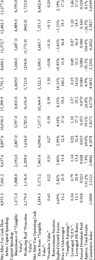
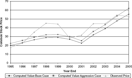
FIGURE 5.1 Coca-Cola: Price versus Computed Value
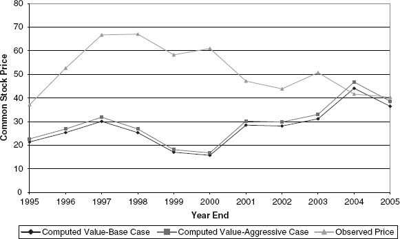
For comparative purposes, we compute per share firm valuations under two different assumptions regarding the estimated long-term real ROE z as described earlier and as shown in Table 5.1. This is the difference between the Base Case and the Aggressive Case in Figure 5.1.
This figure shows that the market price of Coke was substantially in excess of reasonably computed valuations during most of the years under examination. This is certainly consistent with the approximate price-to-earnings (P/E) ratios well in excess of 30-40 during the early part of the period and during the peak of the 1999–2000 market mania.
With the passage of time, the continued growth in core cash flow generation coupled with the underperformance in market price led to conditions at the end of the period where Coke common stock appeared to be reasonably valued in the marketplace relative to its fundamental tangible cash flows and subsequent franchise value potential.
In viewing Figure 5.1, we should take note of a few important methodological items. The actual price series obviously reflects both the company’s financial fundamentals and the market’s evaluation of them. Our computed series, however, essentially holds the fair valuation variables constant, although the computed valuation series reflects the changes in the inflation-adjusted after-tax operating cash flows. As a result, given the fact that most companies experience a significant degree of after-tax cash flow volatility, our valuation estimates exhibit much more variance than in more commonly used dividend discount models (DDMs). This is largely because DDMs have an inherent tendency to start from the smoothest of smooth time series (dividends) and because practitioners typically do not adjust growth rates in the consistent manner described in Appendix A.2
In some sense, our valuation estimates may be a little too volatile since the logical basis of the model presupposes that we are starting with normalized or core operating cash flow (either currently or within a near-term horizon). However, here we deliberately limit ourselves, for demonstration purposes and to minimize subjectivity, to the vagaries that arise in year-to-year changes in reported numbers. We do this with full awareness that such cash flow variances often are not representative of core cash flow changes.
In another sense, though, our valuation estimates are not volatile enough, since we have applied a constant inflation-adjusted, unleveraged discount rate of 6.75% throughout the period. It seems reasonable that this discount rate could change over time, both in the aggregate and for individual companies. Since this discount factor (a) reflects the equilibrating factor between the demand and supply of corporate equities, (b) necessarily reflects the supply and demand conditions of fixed-income investments and other investment opportunities in the economy, and (c) reflects actual and anticipated changes in the taxation of different investments, the discount rate is likely to vary over time.
To deal with this factor, we undertake one other form of analysis whereby we employ equation (4.39) to estimate the discount rate implied by the actual market prices, the observed operating cash flow, the investment ratio, and the projected productivity of investment opportunities. For convenience sake, we have repeated the equation:
This depiction will be most valuable after we have considered the other companies in our case studies. Therefore, we come back to a charting of these estimates a little later on.
Referring back to Table 5.1, we note that Intel experienced very substantial cumulative growth in cash flows, market price, and dividends. Table 5.3 indicates that cash flows for capital spending and cash flows from operations reflected the archetypal boom-and-bust pattern for tech companies in the mid- to late 1990s. The market price, not surprisingly, was even more volatile than the company’s financial and operating results.
TABLE 5.3 Intel Year-by-Year Analysis (amounts in $Millions, except per share amounts)
After the retreat in financial results from the 2000–2001 pinnacle, Intel’s results still recovered strongly in due time and, at the end of the 10-year period, were markedly ahead of the starting point. In fact, on a cumulative basis, after-tax inflation-adjusted cash flow from operations grew at a compounded rate of 7.1% per year over the decade examined. This growth is well in excess of the core growth rate we derive from applying the average reinvestment ratio f and the presumed profitability of reinvested capital z.
Such a divergence between computed inflation-adjusted core growth rates of 3.2% to 3.5% and the realized 7.1% demands an explanation. Recalling that we are practitioners first and financial theoreticians second, our first step is to measure how much of the growth is attributable to the change in effective income tax rates over the period. As it turns out, the change from an effective income tax rate of 36.8% at the beginning of the period to the 31.3% realized in the terminal year has a significant impact. In fact, if you assumed that the final-year tax rate was the same as in 1995, the annualized growth rate of after-tax inflation-adjusted operating cash flow is reduced by almost one full percentage point.
Tax rate changes from year to year, for any given company, reflect the timing of certain tax credits, the resolution of certain classification issues with tax authorities, and certain other discretionary acts by corporate management. More important are the changes in tax law and tax rates and the business growth that happen in nations having a higher or lower effective tax rate than in the United States. (We return to the subject of tax rates in more detail in Chapter 7 and Appendix H.) During the period in question, Intel benefited from a lowering of statutory tax rates in the United States and overseas. It also benefited from shifting much of its production into lower-tax nations.
This explanation helps a little, but we still have to explain the difference between a forecasted core growth rate of 3.2% to 3.5% and an actual, approximate, 6.1% adjusted rate.
Recalling our model’s basic premises, two key points come to mind. First, the inflation-adjusted cash flow from operations in any given year, XT, is a random variable and will reflect changes in product demand and pricing, cost of production inputs, technological change, competitive conditions in the industry, business cycles, and so on.3 Likewise, the profitability of capital expenditures z is also a random variable. During the 10-year period examined, the explosion of demand for microcomputers and related electronic equipment was accompanied by technological advances in manufacturing technology and economies of scale. A sufficiently farsighted investment analyst in the mid-1990s might have performed a prospective analysis by carrying out a projection along the lines of equation (4.41). This analyst would have forecasted several years of cash flows and profitability of capital z above normal conditions before projecting a reversion to a steady-state real-growth model.
The second theoretical factor for explaining growth rates above reasonable core levels is much more subtle. It is the difference between organic and “acquired” growth. As a pedagogical example, suppose some firm entered into several business combinations where it remained the legal successor company. In measuring the growth of cash flows, we would be grafting on the cash flows from the acquired businesses, the impact being potentially to rack up some fairly impressive aggregate growth rates of operating cash flows.4 Of course, on a per share basis and in the capital markets, this impact could be insignificant or even detrimental to the acquiring firm, depending on the terms of the acquisitions.
Note that this second factor did not play much of an apparent role in the Intel history under examination. However, as a general rule, this survivorship bias will almost always tend to produce historical realized growth rates for any acquisitive company in excess of the computed core growth rates that are needed prospectively to be consistent with aggregate economic growth and NIPA statistics. (Chapter 6 covers the implications of large corporate acquisitions.)
Our valuation estimates for Intel are graphically displayed in Figure 5.2. The same basic method was applied as with Coke, namely a 6.75% inflation-adjusted discount rate for the unleveraged firm, the actual debt and shares in place at each year-end, and the growth factors as set forth in Table 5.1. (In all of our case studies, the market prices are adjusted for all share splits occurring over the period.)
FIGURE 5.2 Intel: Price versus Computed Value
The actual share price began the period as significantly undervalued before rising to a level well in excess of “fair value,” even after taking into account the very rapid growth in cash flow early in the period. This situation was not atypical of the market bubble of the late 1990s, a bubble that was especially pronounced in the technology sector. Both the market price and cash flows subsequently pulled back sharply after peaking in 1999–2000.
The astute reader will quickly note that the fair value estimates in the model are essentially unchanged during these three years. Once again, the practitioner’s instinct is on display. This is because, as can be seen in Table 5.3, the actual operating cash flows appeared to be exaggeratedly high in 2000 and exaggeratedly low in 2001. In order to do our retrospective analysis, we took a little artistic license by utilizing an average of 2000 to 2002 cash flow in our valuation estimates for that period. Thus, the volatility of the computed values is admittedly an artificial value of zero. I believe, however, that, even in real time, astute analysts recognized and adjusted for what was more likely to be a “normal” or sustainable level of cash flows during this period.5
Intel’s operating cash flow recovered from its lows with the end result being the strong cumulative 10-year growth discussed earlier. The retreat of the stock price from unjustifiably high levels, coupled with this recovery in operational cash flow, produced a situation at the end of the period where price was once again below computed valuation.
Recapitulating, from 1995 to 2005, Intel outperformed market indices despite the tech stock collapse midway through. In the final analysis, this performance reflected a combination of strong cumulative underlying cash flow growth from operations and a move from significant undervaluation at the beginning of the period to less sizable percentage undervaluation at the end. Interestingly, because of the very solid growth in Intel’s business, the stock would have achieved about an 11%+ annualized total compound return over the period if it had done nothing more than sell at a price equal to the base case valuation estimate at each point in time. The difference between this return and the actual 13.8% compound annual return is a measure of the impact of moving from deeply undervalued at the beginning of the period to much less undervalued by the end.
Referring back to Table 5.1, it is apparent that P&G was a success story by almost any standard during the period studied. Its growth rates of inflation-adjusted operating cash flow strongly outpaced those of Coke, the other consumer nondurable company in our group. In fact, such profitability even outpaced Intel in what was cumulatively a very favorable period for tech companies.
Table 5.1 also displays P&G’s enviable 13.5% cumulative annual total market return during the period. Table 5.4 helps us analyze why P&G’s financial results surpassed even tech company Intel but also why P&G’s cumulative market performance did not quite match up with Intel.
TABLE 5.4 Procter & Gamble Year-by-Year Analysis (amounts in $Millions, except per share amounts)
By now, we are accustomed to investigating first the impact on cash flow attributable to the secular decline in corporate tax rates in the United States and internationally. A rough estimate is that the decline in tax rates contributed about 0.6% per year to the compound growth rate over the decade. This figure still leaves us with an approximate 7.5%/year inflation-adjusted growth rate to dissect.
The same factors mentioned in the Intel study manifest themselves here. The actual return on capital investment appeared to deviate positively versus a normalized estimate of such z. In addition, the actual extent of capital investments and, in P&G’s case, purchases of intact businesses was above what constituted a long-term normal estimate for f. The big factor, though, is that operating cash flows, XT, were subject to several positive shocks during the period. In slightly different terms, the tangible value component of P&G’s business outperformed expectations, in part due to the steady internationalization of P&G’s businesses that led to sales growth well in excess of demographic potential in the United States. Our parting word on the subject is to reemphasize the point made with respect to Intel: The acquisition of intact businesses has the inherent tendency to produce historically observed operating cash flow growth trends above and beyond a sustainable, forward-looking organic growth.
In estimating a sustainable cash flow growth factor, as summarized in Table 5.1, we utilized a reinvestment factor f of .3081, which is below a value of .48 that would obtain had we counted all major business acquisitions as capital expenditures. Instead, once again, we took a practitioner’s approach by assuming major business expansions were twice what would normally be expected during the period in question. Utilizing an f factor of .48 would lead to an unrealistically high ≈5% core growth rate to perpetuity. While this might be a logical interim growth rate, in the context of equation (4.41), such a high inflation-adjusted rate to perpetuity cannot be reasonably supported even by the demographics of P&G’s continued foreign expansion.
As we discuss more in Chapter 6, the larger the purchase of an intact company, the more the transaction will be in the nature of a financing transaction and the less it will be operational in nature. In other words, a merger or acquisition of a sizable company is likely to be on the terms of the market’s prevailing discount rates rather than subject to the investment potential z of capital expenditures within a company. Acquisitions of intact businesses raise potential difficulties that are larger than the normal-course-of-business capital spending by a firm. In concrete terms, acquisitions of intact business units entail more complexities with regard to human resources, regulation, antitrust law, and so forth as compared with normal capital spending within a company’s operating footprint. It is possible that four sizable, successful business unit purchases could well be canceled out by failure of the fifth. This is another way of saying that the average z for intact business unit purchases could lag behind those of internally generated capital spending and product development opportunities.
The success of P&G’s four sizable business unit acquisitions during the decade certainly beat the odds of what corporate America typically experiences. P&G’s next “roll of the dice,” the acquisition of Gillette Company, is examined in Chapter 6.
In concluding this case study, we turn to Figure 5.3, which displays the behavior of P&G’s common stock price as compared with two computations of model valuation. P&G’s stock price appeared undervalued throughout most of the period but tended to track our value computations more closely over the decade than in the case of the two companies we previously analyzed. Interestingly enough, the relative magnitude of market undervaluation was approximately the same at both the beginning and the end of the decade under examination. As a consequence, the superior market performance is directly attributable to the company’s superior financial/operating performance relative to core expectations.
FIGURE 5.3 Procter & Gamble: Price versus Computed Value
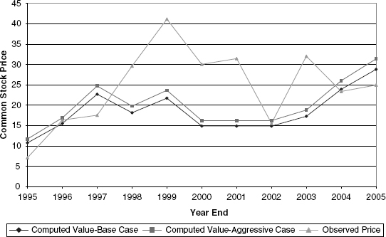
MARKET-IMPLIED, INFLATION-ADJUSTED DISCOUNT RATES FOR COCA-COLA, INTEL, AND PROCTER & GAMBLE
As promised, here we present in Figure 5.4 a valuation estimate under somewhat different assumptions, as discussed under our case study of Coke. We attempt to estimate the inflation-adjusted discount rate for the unleveraged firm utilizing our estimates of the core growth rate of cash flow, the normalized capital reinvestment ratio, and the observed values of operating cash flow and market prices of the firm’s securities. (The core growth rates are consistent with the “Base Case” estimates in this chapter’s figures that compared market prices with computed valuations.)
FIGURE 5.4 Comparison of Real, Unleveraged Equity Discount Rates
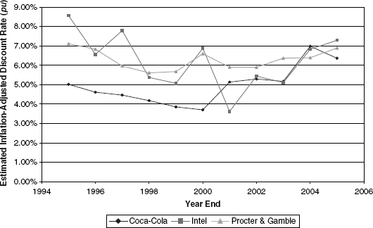
The implied discount rate has the potential of being a highly useful tool for both security selection and asset allocation. Its usefulness stems from the very high sensitivity of equity market valuation to changes in the inflation-adjusted discount rate. (The reader may revisit this in Chapter 3 and/or Appendix C.)
Whenever we see a decline in the discount rate over time, it is keying us to the fact that the observed stock price is benefiting from an ultimately nonsustainable factor. Under reasonable conditions of financial market equilibrium, the discount rate cannot continue to decline period after period. Likewise, an increase over time in the discount rate alerts us that the stock price is suffering from what is most likely a nonsustainable factor. We emphasize again that this is because we believe that our core growth rate expectations are reasonable by macroeconomic and microeconomic standards and that the securities markets are robustly moving to value securities on a prospective risk-return basis over the long run.
Although we do not have a systematic theory of what the appropriate discount rates “should” be in financial market equilibrium, we can utilize historical data and comparisons between similarly situated firms to give us a useful framework for securities selection. A comparison of two global consumer products firms, Coke and P&G, can make this more concrete.
At the outset of the period, our estimates of sustainable growth rates implied that P&G’s expected unleveraged discount rate was better than 200 basis points above that of Coke.6 Consequently, if operating cash flow performed according to estimates, an investor in P&G would expect to earn this additional premium over Coke every year in perpetuity . . . or else expect that at some point in the future, P&G’s stock price would significantly outperform Coke’s to bring the then-prospective returns into an economically reasonable risk/return relationship.
Relative differences in operating cash flow growth could distort these results in actual practice. In our example, P&G’s corporate financial performance was much better than Coke’s in the period studied. Thus, the P&G/Coke stock price performance gap grew even more.
The “irrational exuberance” of the late 1990s is evident in all three discount rate series trending down.7 Poor absolute stock market price performance is evident in the spikes upward in the discount rates. Of the three companies presented, P&G appeared to be least prone to market irrationalities throughout the period. At the end of the period, on both a relative basis and an absolute basis (i.e., as measured by the historically observed approximate 7% real risk premium on unleveraged equities), valuations for Coke and Intel appeared much more reasonable than either at the beginning or at most points along the way.
The case of Enron puts our model to the test in many ways. It is presented here to point out that all models have inherent limitations and that the practitioner’s judgment is indispensable. It also shows just how much a puzzlement certain anomalous cases can be.
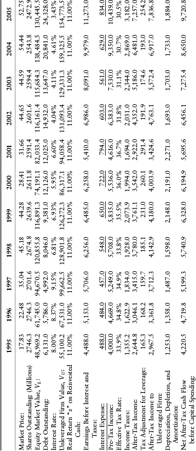
From beginning to end, the case of Enron has frankly stumped me. From the mid-1990s to the end of the decade, I was never able, in real time, to understand why Enron sold at the seemingly rich valuations it did, both in the equity market and in the debt markets. Furthermore, in mid-2001, I was beginning to formulate and collate many of the ideas that are now presented in this book. My preliminary results were consistent with the formal results provided later: On a sustainable basis, Enron appeared to have tangible value late in 2001 even while the actual market price was headed rapidly toward zero. In any event, I had the good sense not to purchase Enron early on and the good luck not to buy it later. The details of the analysis are shown in Table 5.5.
TABLE 5.5 Enron Year-by-Year Analysis (amounts in $Millions, except per share amounts)
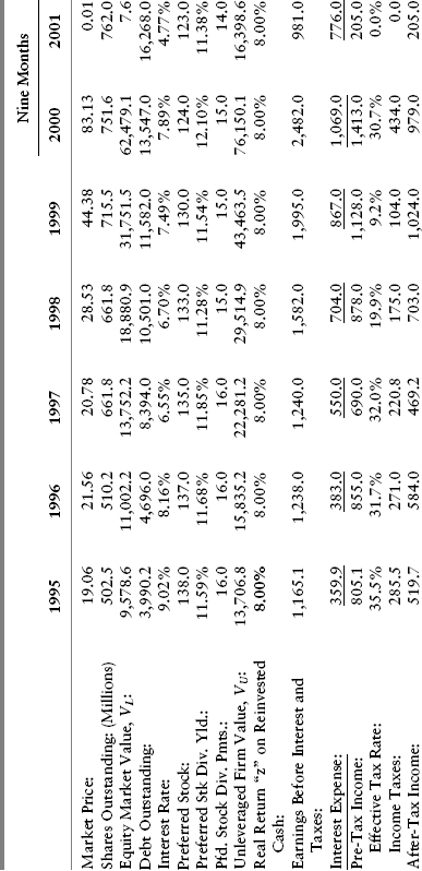
There are several differences in Enron’s financial profile compared with the other three cases we have examined. The first thing to notice is that the ratio of capital spending to current-period operating cash flow aggregated well over 100% during the period in question. In fact, during several years, the ratio was a multiple of operating cash flow. Two types of companies typically exhibit this type of cash flow profile: utility companies undergoing periodic capacity construction programs and start-up companies in the ramping-up part of their life cycle. This presents us with our first set of practical difficulties: What do we utilize for the real ROE z and how do we implement our valuation formula with a reinvestment ratio f of over 1.0?
Enron’s business throughout the period included several natural gas pipeline companies where the achievable return on invested capital (known as rate base under utility ratemaking principles in the United States) is constrained by regulation. A rough attempt to deal with this, and which I recommend for use when analyzing plain-vanilla utility companies, is to utilize an inflation-adjusted ROE z that approximates the unleveraged, inflation-adjusted discount factor ρU. This is a way of dealing with the fact that capital-intensive, regulated entities usually are constrained in profitability over time to amounts comparable to their after-tax weighted cost of debt and equity capital.
In Enron’s case, a substantial amount of capital was also invested in nonregulated assets, many of them well outside Enron’s area of core expertise and many even outside the Western Hemisphere. This was the portion of Enron’s business that had the characteristics of a start-up company, especially in that many of its investments were in recently deregulated electric power markets (domestically and abroad) and in technologically new areas, such as fiber optic cable.
Our practitioner’s approach in dealing with these moving parts was to implement a real profitability factor z that would average out the different profitability expectations for both its regulated and nonregulated business lines. This explains the difference in z compared to Coke, Intel, and P&G. (In real time, a weighted average z could be computed; in our retrospective case, we obviously used a rounded number.) In addition, in dealing with either a utility-type company or a high-growth company, we typically need to avail ourselves of equation (4.41), whereby we project “by hand” the next several years of net cash flows together in conjunction with projecting a steady-state situation, that is, f < 1.0 is reached at the end of the forecast horizon.
Before commenting on the valuation results, it also important to note the substantial swings in Enron’s effective income tax rates, particularly as the company approached its insurmountable problems. These swings, along with the very substantial pace of dollar investments in areas outside its core competency, were certainly warning signs to investors with a cautious bent.
The results of our valuation estimates are presented graphically in Figure 5.5. The Base Case Valuation reflects an assumed normalized f = .4, a z = 8.00%, and ρU = 6.75%. The Special Case Valuation utilized these basic assumptions for the horizon year while utilizing manual estimates of operating cash flows and capital expenditures in the near-term years. In essence, the Base Case Valuation is in the nature of a reality check for our near-term manual inputs.
FIGURE 5.5 Enron: Price versus Computed Value
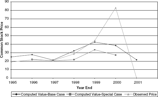
In 2001, the company retroactively adjusted the financial statements and presented in order to deal with off-balance-sheet partnerships. The results in the figure reflect the original numbers, not the subsequent readjustments. Interestingly enough, the dollar magnitude of such adjustments was small enough that Enron still had substantial computed value toward the end of its corporate life in late 2001.
According to our valuation estimates, Enron appeared to be undervalued during the first few years. Although not presented here, lower estimates of the real ROE z might have then been more appropriate, given the regulated nature of Enron’s investments. Even in the emerging unregulated power markets, it would be unreasonable to forecast returns on capital much greater than achieved under a regulated regime. Making a conceptual adjustment of this nature would produce a lower computed valuation; in other words, our cash generation estimates for Enron are probably quite generous. In any event, the market price far outran any reasonable value estimate during 2000 and into 2001.
The big challenge to our model is why it produces a value so far above Enron’s completely vanishing price as of the end of 2001. Part of the problem is that the model is dependent, at any point in time, on an assumption that financial information is being presented fairly and accurately. I believe that core cash flows and asset valuations were not as dismal as the market came to believe in the frantic days of 2001 (in the aftermath of the California power market upheaval and the terrorist attacks in New York and Washington). However, the off-balance-sheet partnership loans, which were collateralized with Enron common stock, induced a liquidity squeeze by lenders. Each tick down in the price contributed to a snowball effect, compounding the stock price decline and further spooking creditors. Once bankruptcy occurred, operating assets ultimately were liquidated at what was, in retrospect, very much the low point of the energy market.
The moral of the story is that a computed value may have been reasonable, but such a model works only on the assumption that no going-concern anxieties exist in the minds of lenders and that no ratings triggers or other mark-to-market accelerators of debt maturities are operating.
TYING UP THE PACKAGE: PRACTICAL LESSONS FROM ALL FOUR CASES
It is difficult to estimate the correct fair value for any company at each point in time. However, the common thread of all four cases is that a little common sense and some reasonable fundamental corporate cash flow and historical valuation parameters would have provided useful information for portfolio rebalancing. I would not propose a robotic binary rule based on buying when a stock is undervalued and selling when it becomes overvalued. However, allocating increasing amounts to ownership positions would be logical the greater the price appears to lag relative to the historic valuation estimate. Likewise, allocating away from stocks would tend to be profitable the greater the market price becomes relative to historic measures of fair valuation.
Finally, as the Enron case study showed, our system still could get us into danger if we do not pay proper heed to the speed at which a stock price falls relative to fair value. In other words, we are always well advised to take our own models with copious grains of salt.
1 For comparison purposes, we utilize the same assumed inflation-adjusted ROE for Coke, Intel, and P&G. (Enron is treated differently for reasons that will be explained in the text.) The reasoning is that the real ROE z is not likely to be noticeably different for similarly situated companies in a competitive market economy. Rather, I think differences in core growth rates are more likely to be attributable to differences in the availability of positive net present value (also known as franchise value) investment opportunities. In other words, differences in growth rates between firms are assumed to be primarily due to differences in f rather than differences in z. While this is not precisely true, it is a robust operational approach, as the examples show. For sensitivity purposes, we also compute core growth rates utilizing a real ROE that is 100 basis points higher (i.e., z = 12.0%). Given the historical ratios of f in the U.S. National Income and Product Accounts, in order to match the historically observed growth of real profits, a real ROE in the neighborhood of 10% to 11% appears reasonable.
2 DDM valuations are also subject to the fact that practitioners do not always systematically adjust the leveraged discount rate to take into account its high sensitivity to the debt ratio of the firm and thus to its future debt financing and common stock issuance/repurchase strategies.
3 In the Leibowitz paradigm, this variation of XT implies that both tangible value and franchise value components of a firm’s value are random variables that evolve over time. There is nothing “fixed and constant” about tangible value, as any buggy-whip or vacuum tube maker will tell you—if you can find one.
4 The opposite happens in the case of a corporate sale or divestiture of operations.
5 The reader may take some additional comfort knowing that the market prices for Intel still greatly exceeded the computed values even when the actual cash flows in this period were utilized. The reader may also wish to refer back to the discussion in the Coca-Cola case regarding the dangers of robotically utilizing actual cash flow in any given 12-month period.
6 The differential leverage in the capital structure would result in a slightly higher expected return to the actual equity shares held by P&G as implied by equation (4.38B).
7 In the case of Coke and other market favorites, the observed risk premiums for unleveraged equity appeared to be insignificantly different from the corporate-debt-to-inflation risk premiums prevailing at the time; this was yet one other valuation “smell test” that hinted at danger.