
CHAPTER 10
Selecting among Efficient Portfolios and Making Dynamic Rebalancing Adjustments
Modern academic approaches to portfolio selection typically have started with the bedrock question of how investors evaluate and choose among the uncertain consumption—or cash flow—streams represented by differing investment securities. This is the conceptual equivalent to what is referred to in other areas of finance and econometrics as a structural model. For our purposes as practitioners, we may utilize a method that is similar to what finance and econometric specialists call a reduced-form approach. With this approach, we do not dig all the way down to the foundation. Rather, we assume that tractable, mathematical rules for choosing among portfolios are given and that such rules are reasonably consistent with observable value-maximizing behavior by investors.
Our reduced-form ranking method can be typified by the general equation form shown in equation (10.1),
where
U = a measure of portfolio desirability
R = expected portfolio return
σ = portfolio risk as measured by standard deviation
e = base of the natural logarithm
K, ε, and α = positive, scaling constants
The relationship between portfolio desirability and expected return is reflected in the partial derivative of U with respect to R.
The mathematical meaning of this partial derivative is that increasing expected return, R, will always increase portfolio desirability, U, for any given risk level, since all the terms in the equation are positive.
It is worthwhile to calculate the second derivative of equation (10.2) to see how this positive relationship between portfolio desirability and expected return changes as we continue to vary expected return. This results in:
If we make the reasonable assumption that 1 > ε > 0, then equation (10.3) will always be less than zero. This is intuitively sensible since it would mean that, for any given level of risk, adding the next 100 basis points to expected return does not increase portfolio desirability as much as did the preceding 100 basis points. (This is the law of diminishing marginal utility in portfolio guise.)
We can assess the impact on portfolio desirability from changes in risk level in a manner similar to our investigation of expected return. Taking a partial derivative with respect to standard deviation, we obtain:
As long as the scaling constant α > 0, the desirability of any portfolio will be negatively impacted by an increase in the standard deviation when the expected return is held constant.
For the second partial derivative, we can see how the relationship between desirability and risk changes as risk continues to increase. The specific equation is:
The relationship is positive, although it is probably best not to read too much into this particular result. What this relationship is really saying is that portfolio desirability can never fall into negative territory.1
We next undertake an exercise that is familiar from basic microeconomics. Specifically, we assume that there is a given level of portfolio desirability, call it U″, and that we would like to see how different combinations of expected return and risk can achieve such a level. The curve that maps out this constant level of portfolio desirability is called an isoquant in technical terms and can be compared with other isoquants, say U″′ or U′, having, respectively, either higher or lower constant levels of portfolio desirability.
Figures 10.1, 10.2, and 10.3 present a comparison of portfolio desirability curves among three distinct economic agents with differing propensities for risk bearing. The first figure gives an example for a highly risk-averse investor or, stated alternatively, an investor with low risk tolerance.
FIGURE 10.1 Portfolio Desirability under Low Risk Tolerance
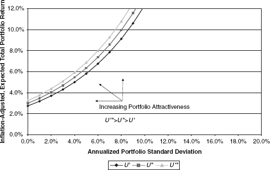
FIGURE 10.2 Portfolio Desirability under High Risk Tolerance
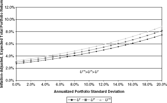
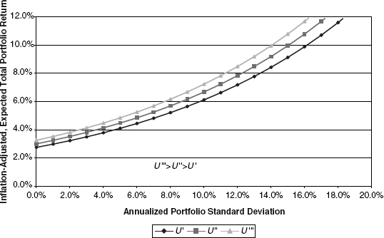
FIGURE 10.3 Portfolio Desirability under Medium Risk Tolerance
The next example is of an investor that is far less risk averse, that is, one with high risk tolerance.
In both of these figures, risk-averse behavior is demonstrated insofar as higher expected returns are necessary to induce investors to hold successively more volatile portfolios. Furthermore, all curves are positively concave, meaning that the reward must rise at an increasing rate the more the standard deviation is increased. In comparing the two figures, it is evident that the more risk-tolerant investor requires much less reward as compensation for assuming additional portfolio volatility.
For purposes of creating a full perspective, Figure 10.3 reflects an investor with risk tolerance somewhere between each of that shown in Figures 10.1 and 10.2.
To complete the theoretical discussion of portfolio ranking and selection, it is useful to establish additional mathematical foundations. Along any given isoquant U (i.e., for any given investor), the expected return and risk combinations must be such that the relationship shown in equation (10.6) holds:
It is a manner of simple algebra to transform this into equation (10.7):

In nonmathematical language, equation (10.7) states that the slope of the portfolio desirability isoquant, at each and every point, is the ratio of the marginal disutility of risk divided by the marginal utility of expected return.
RECONCILING PORTFOLIO DESIRABILITY AND FEASIBILITY
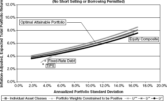
The next step is to merge the analysis from Chapter 9 with the portfolio selection criteria just established. The best place to start is with a visual depiction of the process. Figure 10.4 overlays the portfolio selection functions for the investor depicted in Figure 10.3 with the feasible (and efficient) portfolios constructed in Figure 9.11.
FIGURE 10.4 Optimal Portfolio Choice: Medium Risk Tolerance Investor
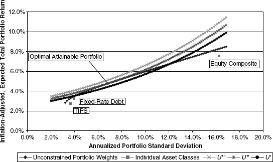
To understand why the specified intersection point in the figure is labeled as the Optimal Attainable Portfolio, it is useful to consider why other points are not optimal and attainable. Starting with the latter is easy, since it is evident that any portfolio desirability curve—or isoquant—lying above the efficient-portfolio set (denoted by the diamond-symbol line) can never be reached. Let us thus now consider two portfolios that are attainable but not optimal. For instance, the portfolio desirability isoquant labeled U′ intersects the efficient-portfolio curve at two points. One intersection is at a point of low risk and low expected return; the other is at a point of higher risk and higher expected return. Since they both lie on the same isoquant, the investor would be indifferent between holding either portfolio. However, the investor can plainly better him- or herself by moving from either point along the efficient-portfolio curve toward an interior point in order to reach an isoquant with a higher level of desirability. (In three dimensions, moving from the two initially assumed intersection points toward the middle of the efficient-portfolio curve represents a climbing of the portfolio desirability hill.) By carrying this pictorial logic to its conclusion, the optimal attainable portfolio must be the one where the slope of the efficient-portfolio curve and the best attainable isoquant are equal, that is, where the two curves are tangent to each other.
As it turns out, what we see is what we get. The next mathematical development establishes this result formally. (The less mathematically inclined reader may choose to skip to the next section.)
![]()
Subject to: R = h (σ) or, alternatively, R − h (σ) = 0 (where R = h (σ) represents the efficient-portfolio curve determined from the equations in Chapter 10).
Utilizing the by-now familiar LaGrange method for constrained optimization, we obtain the solution system:
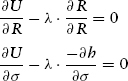
From the first of the two equations, it can be seen that:
Consequently, substituting ![]() into the second part of equation system (10.8) produces:
into the second part of equation system (10.8) produces:
This equation can be readily transformed into:

Finally, making use of the result from formula (10.7), we get the promised result that the optimal attainable portfolio is where the slopes of the portfolio desirability isoquant and the efficient-portfolio curve are equal, namely:
TURNING THEORY INTO EASILY CALCULATED RESULTS
It is not difficult to ascertain the slope of the efficient-portfolio curve at each and every point. For the classical case where portfolio weights are permitted to be negative, the closed-form equation can be found in Appendix J, formula (J.13). Where portfolio weights must be nonnegative, we still can compute the slope of the efficient-portfolio curve numerically at any point—to any arbitrary degree of precision—simply by finding the risk/return coordinates for any two sufficiently close points and numerically computing the slope between them. In other words, obtaining the right-hand side of equation (10.12) is not difficult regardless of which case applies.
What we also desire is a sufficiently easy method for obtaining the left-hand side of equation (10.12). As it turns out, one of the advantages of our formula (10.1) for portfolio desirability ranking becomes apparent when we take the partial derivatives indicated in equations (10.2) and (10.4) and substitute them into equation (10.7). The first step is thus:
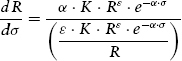
which simplifies, through cancellation of terms, to a simple and highly useful result:
It is a matter of trial and error to obtain the specific R that causes equation (10.14) to equal the slope of the efficient-portfolio curve, ![]() .2 (This is a pragmatic approach as compared with the differential equation technique that would otherwise be needed to solve the system directly.)
.2 (This is a pragmatic approach as compared with the differential equation technique that would otherwise be needed to solve the system directly.)
With our methodology thus established, it is a straightforward computational matter to obtain optimal portfolio selections for the cases of low and high risk tolerance, respectively. Examples are shown in Figures 10.5 and 10.6, which reflect the same scale and portfolio inputs as the other figures in this chapter.
FIGURE 10.5 Optimal Portfolio Choice: Low Risk Tolerance Investor
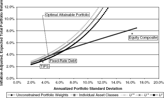
FIGURE 10.6 Optimal Portfolio Choice: High Risk Tolerance Investor
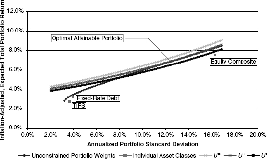
The next logical question relates to the impact on optimal portfolio selection arising as a consequence from the constraint that portfolio weights be nonnegative.3 In principle, there is no difference in the method by which a portfolio is selected from this more constrained set of efficient portfolios. In fact, as we saw demonstrated in Figure 9.11, the efficient-portfolio curves, both with and without the positivity constraints, typically will coincide at medium and lower volatilities. Not surprisingly, for investors with low and medium risk tolerance, it is easy to imagine that the positivity constraints are not binding under normal conditions. In other words, the constrained and unconstrained solutions will be the same or will differ very slightly for these investors. For the more risk-tolerant investors, however, positivity constraints are very likely to lead to different portfolio configurations, as shown in Figure 10.7.
FIGURE 10.7 Constrained Optimal Portfolio Choice: High Risk Tolerance Investor
In Figure 10.7, the expected optimal portfolio to a highly risk-tolerant investor is noticeably lower than in the previous case in Figure 10.6, where such nonnegativity constraints did not apply. The resultant optimal portfolio standard deviation also is lower than in the previous comparison case. There is nothing surprising about this result. After all, when investors face the prospect of less of a reward for bearing risk, it stands to reason that they will choose to accept less of it.4
ADJUSTING FOR CHANGES IN LONG-TERM EXPECTED RETURNS ON COMMON EQUITY
The treatment has so far been familiar to theoreticians and practitioners alike. Usually the analysis stops at this point, and the prescriptive recommendations are for target portfolio weights that are suitable to investor risk preferences under the assumption that the efficient-portfolio set does not change enough to warrant significant portfolio rebalancing. However, if our equity-valuation model gives us valid insight into changes in expected equity returns, it seems worth investigating how to make best use of such information. We can start by investigating the impact where expected, inflation-adjusted equity returns vary, holding expected returns on Treasury Inflation Protected Securities (TIPS) and fixed-rate debt constant.
In order to facilitate such analysis, we designate the efficient portfolio curves (both with and without positivity constraints) as either Case 1 or the Base Case interchangeably. In this section, we examine two cases in which the long-term expected returns on common equity are higher (Case 2) or lower (Case 3), respectively, when compared with the Base Case.
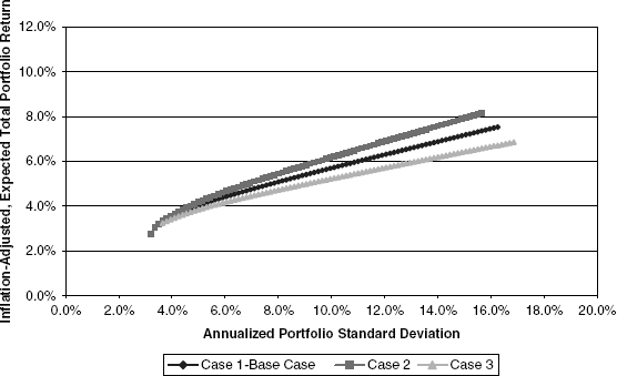
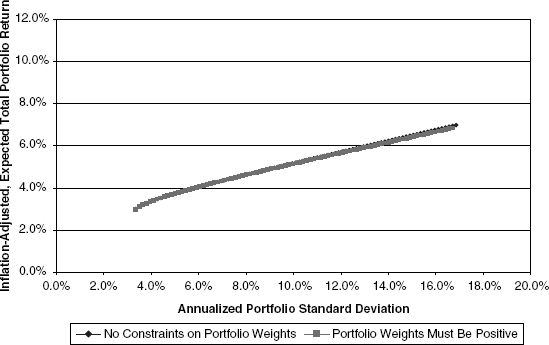
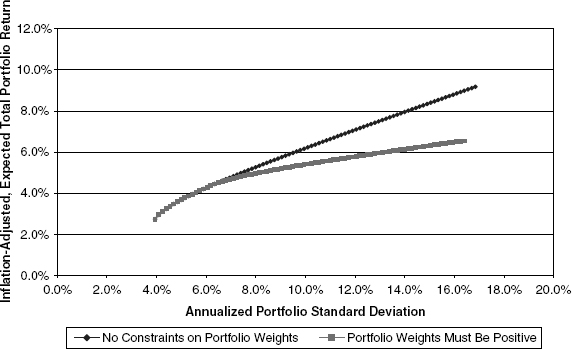
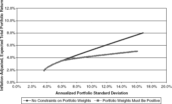
In Figure 10.8, the efficient-portfolio curves are shown for each case under the assumption that there are no positivity constraints on asset weights. Figure 10.9 makes the corresponding comparisons with the requirement that asset weights do satisfy positivity constraints.
FIGURE 10.8 Efficient Portfolio Sets under Different Expected Equity Returns (No Positivity Constraints on Asset Weights)
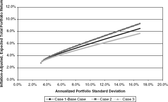
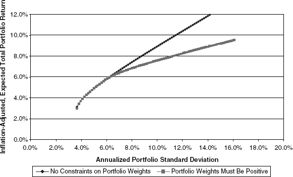
FIGURE 10.9 Efficient Portfolio Sets under Different Expected Equity Returns (Asset Weights Constrained to Be Positive)
Figures 10.8 and 10.9 are drawn to the same scale as the preceding figures in this chapter to facilitate visual comparisons.
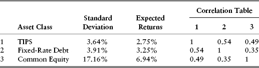
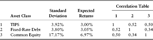
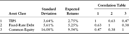
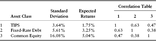
The expected return, variance, and correlation data for each scenario are based on the underlying assumptions set forth completely in Appendix L. For expositional purposes, we summarize the relevant information for each case in Tables 10.1, 10.2, and 10.3.
TABLE 10.1 Case 1 Assumptions

TABLE 10.2 Case 2 Assumptions

TABLE 10.3 Case 3 Assumptions
In addition to changes in the expected returns, Tables 10.2 and 10.3 reveal certain other noteworthy changes compared to the Base Case in Table 10.1. Because the only underlying difference among the three scenarios is the inflation-adjusted equity discount rate, ρU, Case 2 produces a somewhat lower standard deviation for expected common equity returns and Case 3 a slightly higher standard deviation. These results are mildly counterintuitive, since what we often see when stocks are depressed, or “cheap” as in Case 2, is that observed volatility is often higher than historical averages. Similarly, when markets are “rich” by historical standards, observed volatility often appears lower, not higher.
The explanation for these somewhat counterintuitive results lies in equations (8.7) and (8.23), which provide the basic formulas for equity volatility. In those equations, the higher the discount rate, the lower the multiplicative factor applying to the volatilities of each of the underlying valuation factors. (The reader is advised to scan the equations again to verify this.) The reverse happens when the discount rate is lower. Since we wanted to isolate the impact of discount rates only, we deliberately kept the assumed debt leverage percentage the same. In actual conditions, higher discount rates (depressed equity markets) usually bring about rising debt ratios, simply due to market declines, thereby tending to counteract the reduction in risk implied by Case 2 in Table 10.2. Correspondingly, lower discount rates (rich markets) have the immediate impact of lowering debt ratios, thereby leading to a volatility-dampening impact vis-à-vis Case 3 in Table 10.3.
(A further aspect of empirical volatility observations is that most equity volatility arises, as we saw in Chapter 8, from changes in the firm’s core cash flow from operations. This, coupled with the leverage impact just outlined, tends greatly to outweigh volatility changes arising from equity discount rate changes.)
The remaining items of interest are in the correlation tables. The impact of changed common equity volatility does have a modest impact on changing the correlation between both TIPS and fixed-rate debt vis-à-vis common equity across scenarios. More important, the correlations are low enough that meaningful benefits arise from asset class diversification.
These changes, taken in totality, produce a counterclockwise rotation of the efficient-portfolio curve in Case 2 and a clockwise rotation in Case 3 as compared with the Base Case. Instead of presenting pictorial representations of the optimal portfolios selected under each case, we present only summary results in Table 10.4.
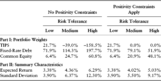
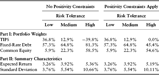
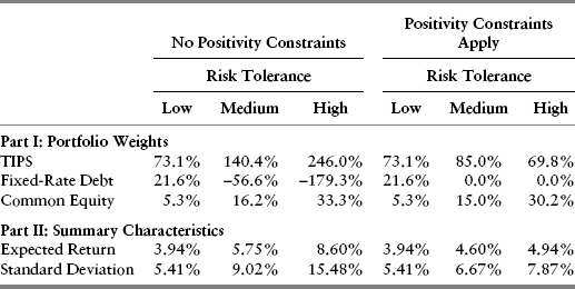
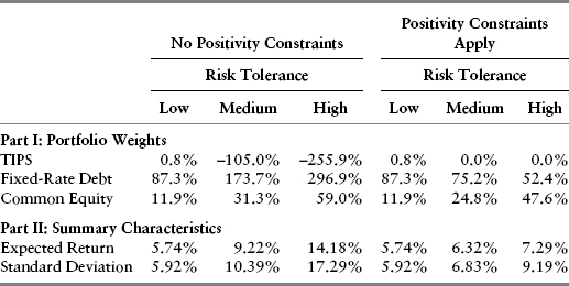
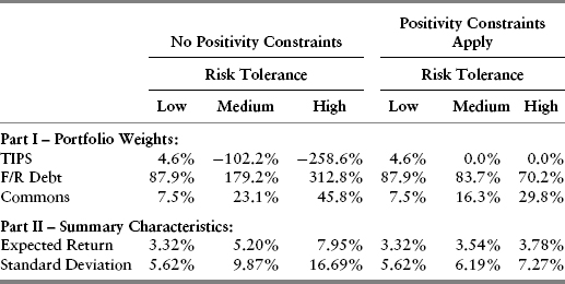
Tables 10.4, 10.5, and 10.6 contain much to digest. The most significant implication is that raising expected equity returns (Case 2) produces upward shifts in the portfolio allocations to common equity, regardless of whether the positivity constraints apply. When equity returns are lower than usual (Case 3), the opposite happens; equity allocations are lower across the board.
TABLE 10.4 Base Case Optimal Portfolio Results
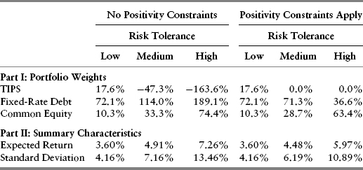
TABLE 10.5 Case 2 (“Cheap Equities”) Optimal Portfolio Results
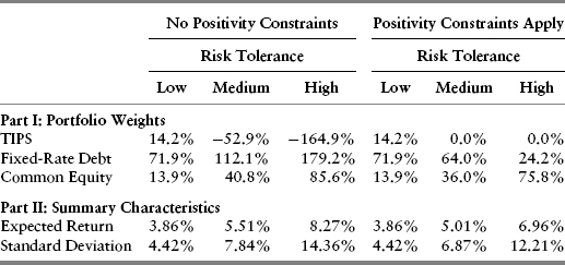
TABLE 10.6 Case 3 (“Rich Equities”) Optimal Portfolio Results
Another interesting implication is that even investors with low risk tolerance will have allocations of ostensibly “risky” common equity and, furthermore, their optimal portfolio allocations will shift in response to changes in the relative expected returns of equity versus debt alternatives.
The other implication, one that neither theorists nor practitioners seem to understand well, is that the responsiveness of asset allocations to changes in expected returns is noticeably greater among investors with higher risk tolerance. The bromides against “excessive turnover” thus actually may do a disservice among those investors—for example, young workers with high incomes—who are capable and desirous of bearing substantial risk but who are deterred by such advice.
Failing to adjust portfolio allocations to changes in relative risk-adjusted returns violates the basic premises of microeconomics. It is akin to buying a fixed amount of apples, strawberries, and oranges every week at the supermarket, rather than loading up on apples in the fall, strawberries in the summer, and oranges in the winter, when each fruit is cheapest.
The conceptual exercise that follows is one of many ways to illustrate the disadvantages of not rebalancing portfolios in response to shifts in risk-adjusted returns. The example in Table 10.7 is for an investor, who faces positivity constraints on portfolio weights and that has high risk tolerance. As shown in Table 10.4, the Base Case weights produce an expected return and standard deviation that we designate as “Ostensible” when either Case 2 or Case 3 conditions actually apply, but where the investor’s portfolio weights and expectations do not track with changed market conditions.
TABLE 10.7 Adverse Impact of Suboptimal Portfolio Rebalancing
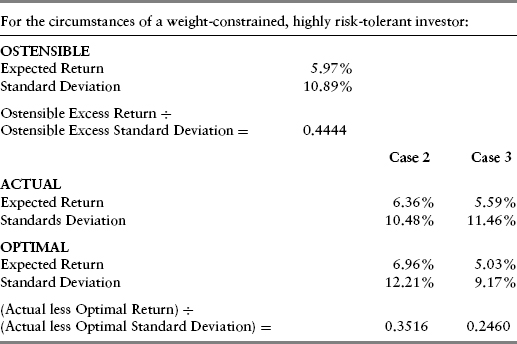
The ostensible expected portfolio return and standard deviation can be compared with the expected return and standard deviation of the lowest-risk asset class, in this case TIPS. Specifically, dividing (a) the excess of the ostensible portfolio return over the excess inflation-adjusted TIPS yield over (b) the excess of the ostensible portfolio standard deviation over that of TIPS produces an ostensible return to risk target. In the case shown in Table 10.7, it is 0.4444. If the investor keeps the portfolio weights the same regardless of whether Case 2 or Case 3 actually prevails, the actual incremental return to risk relationship can be computed by comparing the optimal portfolio to the actual expected returns and standard deviations that would result by applying the Case 1 portfolio weights to the asset returns and volatilities that actually would prevail.
The results show that the difference between optimal and actual results produces a poor incremental return to risk prospect to the degree that the actual portfolio diverges in allocation from the optimal.
ADAPTING TO MORE GENERAL CHANGES IN RISK-ADJUSTED EXPECTED RETURNS
A logical extension of the preceding analysis would be to allow changes in expected returns and volatilities above and beyond those related to common equities. Since the combinations are almost limitless, our demonstrations are limited to four typical cases. (The reader is invited to create additional scenarios as a way of cementing understanding.)
Continuing with our numbering system, our next scenario is labeled Case 4. The specifics are contained in Table 10.8 and we characterize this scenario as being a “toppy” market for equities and fixed-rate debt.
TABLE 10.8 Case 4 (“Toppy” Market) Assumptions
The interesting aspect of this case is that the expected equity return is on the low side and, adjusting for de minimus impacts arising from altered interest cost assumptions, is basically the same as in Case 3. The key differences are that the expected inflation-adjusted return on TIPS is higher and the expected return on fixed-rate debt lower than in the preceding three cases. This pattern typically is seen in late-stage bull markets for equities. Interestingly, the changed discount factors for both kinds of debt have implications on the standard deviations of both debt categories. The standard deviation of TIPS returns rises compared to the Base Case as the higher discount rate, when multiplied by an unchanged volatility factor for percentage changes in real yields, is not offset by a reduction in modified duration.5 For fixed-rate debt, though, the standard deviation is lower, because of a similar impact that lowers volatility of absolute yields via the mechanism of constant percentage yield volatility multiplied by lower absolute discount rates.6
Parenthetically, the impact on relative standard deviations must, of necessity, impact on covariances; the impact shows up in the slightly different correlations versus the Base Case, which are implied by such changed covariances.
Drawn to the same scale as all the other portfolio figures, Figure 10.10 shows cases where portfolio weights are constrained to be positive and where they are not.
FIGURE 10.10 Efficient Portfolio Sets under Case 4 (“Toppy” Markets)
A comparison of Figure 10.10 with the Base Case shows that the efficient portfolio curves virtually coincide for both the constrained and unconstrained sets. More significantly, both curves are higher at low-risk levels and lower at high-risk levels compared with the Base Case. In short, there is less incentive to bearing high risk via large equity holdings. This is precisely what we see when we examine the optimal portfolio solutions for the different investors as depicted in Table 10.9. (The reader will be well served throughout the balance of this section by making frequent cross-reference to the Base Case results in Table 10.4.)
TABLE 10.9 Case 4 (“Toppy” Markets) Optimal Portfolio Results
At the same time, we also see raised allocations to TIPS. The result of these adjustments is that optimal portfolios for all investors reflect noticeably lower risk compared with the Base Case.
The next analytical scenario, Case 5, is characterized as “stagflation.” In this scenario, we subjectively adjust the long-term equity market and fixed-rate debt expected returns downward by 1.0% per year to reflect adverse economic impacts on equity cash flow and, also, adverse impact on fixed-rate debt returns due to heightened inflation. What our subjective forecast effectively says is that both these asset classes are overvalued, although we temper such forecasts to reflect modest annual adjustments toward estimated fair valuation. We temper our forecasts out of epistemological modesty—in other words, we may be wrong—and because the market’s adjustment toward our forecasts may take several years to fully play out.7 We make a similar upward 1.5% subjective return adjustment to annual TIPS returns, since they would be most favorably impacted in a stagflation environment. To reflect fully the heightened uncertainty, we also assume that TIPS yield volatility would be higher under these market conditions. (See Appendix L for full details.)
Our overall Case 5 input assumptions are summarized in Table 10.10.
TABLE 10.10 Case 5 (“Stagflation”) Assumptions
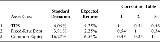
Figure 10.11 presents a visual depiction of these results to bring out the change in relative risk and returns vis-à-vis the Base Case. In addition, Case 5 also presents a stark example of a significant divergence in attainable results depending on whether portfolio weights are constrained to be positive.
FIGURE 10.11 Efficient Portfolio Sets under Case 5 (“Stagflation”)
The portfolio optimization results presented in Table 10.11 show that the optimal results for constrained investors is toward a distinctly low-risk direction as compared with the Base Case. Of interest, however, is the fact that unconstrained investors with greater risk tolerance are well situated to exploit the attractive aspects of TIPS via, in effect, borrowing at a fixed rate and lending at a variable rate. Regardless, in all instances, for both constrained and unconstrained portfolios, the low expected return on equities leads to a marked decline in common equity allocations as compared with the Base Case.
TABLE 10.11 Case 5 (“Stagflation”) Optimal Portfolio Results
The penultimate example, Case 6, represents the mirror image of the stagflation case. We characterize Case 6 as “Supply Side Push” in which an economy-wide improvement in productivity is expected to result in a period of lower measured consumer price growth and improved corporate profitability. Under such assumptions, we subjectively raise the one-year expected return forecasts for both fixed-rate debt and common equity by 2.0%. Our subjective views on improvements to fixed-rate debt valuation
prompt us also to raise slightly the effective volatility of returns for that asset class. Summarizing portfolio inputs, we get Table 10.12.
TABLE 10.12 Case 6 (“Supply Side Push”) Assumptions
These assumptions produce the efficient-portfolio curves shown in Figure 10.12.
FIGURE 10.12 Efficient Portfolio Sets under Case 6 (“Supply Side Push”)
This picture, together with the underlying assumptions, implies that investors are likely to raise their exposures to fixed-rate debt and equity significantly as well as to assume more risk in the aggregate, owing to the healthy incentives for assuming more risk.
The actual “Supply Side Push” results in Table 10.13, however, show the importance of carrying through all the computations. Despite the fact that the expected returns to common equity are well above the Base Case, the common equity allocations among more risk-tolerant investors are actually lower. This situation occurs because risk-adjusted returns on fixed-rate debt are so favorable in this scenario that investors make significant reallocations toward that asset class, in part at the expense of common equity.
TABLE 10.13 Case 6 (“Supply Side Push”) Optimal Portfolio Results
For the sake of balance, we include Case 7, which we label “Deflation.” This case assumes a classic economic contraction where both consumer price levels and business profits diminish. Under these premises, the expected returns on common equities and TIPS are both subjectively lowered (as set forth fully in Appendix L). At the same time, the presumed pressure on corporate debt credit spreads limits the degree of upward tweaking of expected returns on fixed-rate debt while also inducing us to jigger the standard deviation estimate upward for the asset class under this scenario. The inputs are summarized in Table 10.14.
TABLE 10.14 Case 7 (“Deflation”) Assumptions
As has been our practice, we also present Figure 10.13, a graph of the efficient-portfolio curves under these assumptions.
FIGURE 10.13 Efficient Portfolio Sets under Case 7 (“Deflation”)
The declines in risk-adjusted TIPS and common equity returns, as compared with the Base Case, lead us to believe that allocation toward both asset classes will be much lower in the Case 7 Deflation scenario. Table 10.15 shows that this is true and that constrained investors move in the direction of lower overall portfolio risk. For unconstrained investors, however, the ability to exploit the relative return differences between TIPS and fixed-rate debt actually leads to somewhat higher risk portfolios vis-à-vis the Base Case. This situation is entirely logical, given the fairly steep slope of the unconstrained efficient-portfolio curve in Case 7 relative to Case 1. In other words, Case 7 provides better rewards for incurring incremental portfolio risk, and rational investors react accordingly.
TABLE 10.15 Case 7 (“Deflation”) Optimal Portfolio Results
RECAPITULATION AND AN IMPORTANT CAVEAT
This chapter has covered a lot of ground and provided a number of numerical results under different scenarios, constraints, and risk-aversion profiles. It is worth pausing and listing again the generalizations embedded in the individual results.
It is important to rebalance portfolios. Rebalancing asset weights is the optimal way to deal with changes in expected returns and such changes in variances and covariances that arise in connection with these changed return expectations. The importance of rebalancing is true, independent of risk-bearing ability.
The magnitude of changes in portfolio weights is positively related to risk-bearing ability. Investors with the greatest tolerance for risk should be inclined to alter portfolio weights most significantly in response to changes in risk-adjusted expected returns. This is not just good advice for aggressive investors; it is an important value-maximizing strategy for any investor with a sufficient time horizon and an ability to bear risk. A key case in point is for younger investors with high current income from wages or salaries. They are best situated to benefit from disparities in relative expected returns and the most subject to being hurt by a robotic policy of sticking to target allocations regardless of market conditions. This suggested market-responsive rebalancing runs counter to much of the conventional wisdom of our day.
Positivity constraints hurt results. This statement is particularly true for investors with a greater ability to bear risks. While the classical stereotype is that only high-net-worth investors, trust fund babies, and hedge fund gunslingers have high risk tolerance, it is likely that young and middle-age, high-income workers are the main inadvertent casualties of investment restrictions of this sort. In certain markets, the constraints are not terribly binding; in other circumstances, the disparity between the constrained and unconstrained efficient-portfolio curves might be dramatic indeed. (The damage from constraints is exacerbated by the existence of additional asset categories beyond the three that are dealt with in this book.)
Running the numbers is imperative. The risk-adjusted numbers are what drive portfolio allocations, not just changes in the expected returns. Since portfolio optimization is a nonlinear process, it is worth running all the numbers rather than just relying on rules of thumb or intuition.
Understanding the variance/covariance relationships is essential. The valuation model presented in this text is a well-grounded method to reconcile (1) basic economic relationships, (2) historically observed results of underlying valuation factors, and (3) relative expected returns and yields currently prevailing in the marketplace. Computing variances and covariances (or the underlying correlations) from recently observed asset class performance, by contrast, may tend to over- or underestimate correlations. For example, during market crashes and turbulence, the correlations among different asset classes tend to be high. In market bubbles, the correlations may drop to very low levels. Making decisions in light of such transiently measured results tends to result in a lot of buying at tops and selling at bottoms.8
In conclusion, it is important to provide a fundamental caveat. Many readers will have noticed that the portfolio rebalancing principles presented here are essentially contrarian. Holding other factors constant, an asset class almost invariably attains a higher expected return through underperformance relative to other assets, including cash reserves. The dynamic rebalancing principles espoused here will typically involve raising allocations to asset classes that have done poorly and reducing allocations to assets that have performed well.
Carrying out this contrarian strategy consistently is psychologically and sociologically difficult. In discussions of investment results, contrarian investors will have little in common with most of their peers. On average, over time, contrarians will be to them, as Baron Rothschild said in an earlier century, good neighbors, buying assets when acquaintances are eager to sell and selling assets when neighbors are itching to buy them.
The other important aspect of the contrarian caveat is this: Contrarianism is necessary but not always sufficient. Being different does not guarantee that you are right. Our contrarian portfolio rebalancing strategy is not a goose that consistently lays golden eggs. It is much more like having a set of loaded dice. If you keep the bets manageable and stay at the table long enough, you are likely to win a disproportionate number of times. This is not an unrealistic goal for an investor.
1 Expressed more colloquially, there can never be a portfolio such that an investor would be willing to pay for the privilege of extricating him- or herself.
2 This could be done by a look-up table or a goal-seek utility in standard spreadsheet software packages. Alternatively, simple Newton-Raphson–type procedures can be coded into any standard programming language.
3 We succinctly, although imprecisely, occasionally refer to these as positivity constraints in the remainder of the text.
4 In the absence of positivity always weighting constraints, the optimal constrained portfolio will, of logical and mathematical necessity, always be more desirable to an investor than the optimal portfolio where such positivity restrictions apply and are binding.
5 See equation (9.43).
6 See equation (8.20).
7 As seen in the regression analyses of Chapter 7, especially equation (7.4) which implies that a sizable 100 basis point discount rate misvaluation of an individual equity would translate into only 2.7% annual performance differential versus a broad index.
8 Utilizing transient correlations also produces poorly performing hedge ratios for futures/options strategies.