
CHAPTER 9
Constructing Efficient Portfolios
In developing the basic model for equity valuation, we have necessarily touched on the valuation and volatility for both standard and inflation-protected debt securities. We have seen that each of the three asset classes shares both similarities and differences with the other two. Of particular relevance to us, equities are inflation resistant but do not have contractual real cash flows. Treasury Inflation Protected Securities, such as TIPS, are inflation resistant but do not share in the economic fortunes of equity securities. Traditional fixed-rate debt securities do not share in the economic fortunes of the firm but are not inflation resistant. These fundamental dissimilarities provide both opportunities and challenges to us as we attempt to form optimal portfolios.
The focus in this chapter is on allocation among these different asset classes. We assume that the tools for individual stock selection, as discussed in Chapters 4, 5, and 7, are already applied as a prerequisite. This analysis has two major features:
1. Our valuation models give us a robust way of specifying volatility and correlation structure for the three asset classes.
2. We can roughly infer reasonable expected return estimates among the different asset classes.
This second item is particularly relevant for common equity as an asset class because it typically has both the highest expected return and the greatest volatility among the asset classes.
Figures 9.1 and 9.2 bring us to the crux of the equity question. Figure 9.1 presents the interrelationship of expected return and volatility over time for a diversified portfolio of common equities. For the sake of illustration, it is assumed that portfolio returns evolve with a given, instantaneous mean return that is compounded continuously (all income being reinvested in the portfolio). Further, the return process is impacted by continuous, normally distributed random shocks with a constant annualized volatility. In Figure 9.1, we posit a continuously compounded, net of inflation, percentage return, μ, equal to 2.0% per annum and an annualized volatility (i.e., standard deviation of inflation-adjusted returns), σ, equal to 15.0%.
FIGURE 9.1 Example 1: Low Expected Return
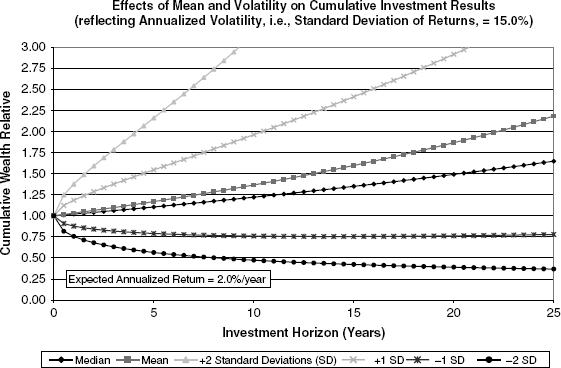
Since the instantaneous percentage returns are assumed normally distributed, the actual cumulative returns, or wealth relatives, will be distributed as normal in the natural logarithms: log-normal. As a result, the wealth relative can never fall below zero while it can theoretically approach infinity. This intuitive explanation leads to a cumulative return distribution that is always positive and with a distinct right-tail skew. It also explains why in Figures 9.1 and 9.2, the mean return, which is weighting some of the very large potential return values, exceeds the median value.
In Figure 9.1, the region between the two lines labeled +1 and −1 standard deviations represents results that we would expect to occur some 68.3% of the time.1 Similarly, the +2 and −2 standard deviation lines enclose a region containing 95.4% of possible results.2 Clearly, as time passes, the range of possible results expands more and more.
Figure 9.2 presents a similar analysis that also assumes the same annualized volatility, α = 15.0%, but where the instantaneously compounded real return on equities is 6.0%. Both figures are drawn to the same scale to reveal how the higher mean instantaneous return produces systematically higher expected cumulative results.
FIGURE 9.2 Example 2: High Expected Return
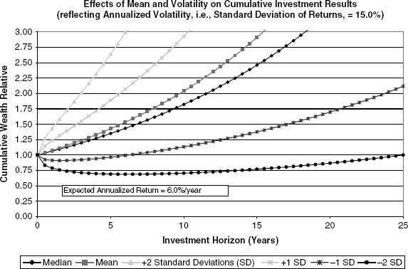
These figures are instructive. For a given volatility, rational investors can easily determine that they would rather have the return process with the higher expected return. In actual implementation, if the expected return process has a low mean value, as in Figure 9.1, investors are likely to attempt to sell off equities and reallocate portfolios to other investment classes until an equilibrium results where subsequent expected compounded return results are higher. Likewise, when expected instantaneous returns are thought to be high relative to volatility, investors will attempt to allocate more of their portfolios into common equities, thereby driving up stock prices until subsequent, prospective returns are reduced.
Academicians have produced several a priori models that attempt to determine what the proper expected return is, given volatility assumptions and the underlying utility functions of the investor population. As discussed in Chapter 8, these models have tended to result in expected return estimates (i.e., equity discount rates) that are only narrowly above risk-free interest rates. While the investment profession awaits further theoretical work to resolve these apparent difficulties, we practitioners need some reasonable quantitative methods to guide us in the interim.
In fact, Figures 9.1 and 9.2 serve as the conceptual springboard for an elegant approach first presented by Robert Arnott in 2004. We have modified the letter of his approach but have followed it in spirit. Thus, instead of imagining an inflation-adjusted return series, as we have already done, we might equally envisage an excess return series produced by the expected instantaneous return of an equity composite less the risk-free rate on debt securities. The resulting wealth relative, under these assumptions, would represent the cumulative over- or underperformance of the equity composite versus the risk-free rate.
We could use these assumptions to create pictures analogous to Figures 9.1 and 9.2 and interpret visually whether the expected return premium was sufficient given the risk of underperforming the risk-free alternative. Alternatively, we could present the data in a slightly different fashion, which we attempt in Figure 9.3.
FIGURE 9.3 Comparison of Expected Results for Different Risk Premiums (i.e., Expected Equity Return less Risk-Free Rate)
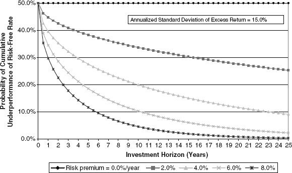
In Figure 9.3, we can balance the impact of expected returns versus volatility by attempting to compute the probability of cumulative underperformance of the risk-free rate over various time horizons. With an expected mean risk premium of zero, Figure 9.3 shows that, over any time horizon, the possibility of over- or underperforming the risk-free rate is a coin flip, 50%. With a positive risk premium, the odds of cumulatively underperforming the risk-free rate are less than 50% and decline consistently with the lengthening of the investment horizon. In fact, if the expected return premium is high enough relative to volatility, the odds of underperformance can shrink very significantly and very rapidly.
Figure 9.3 indicates that, from a practical point of view, it is difficult systematically to posit an 8.0% expected compound return premium versus the risk-free rate because the probability of equity underperformance rapidly diminishes below 10% and tends toward zero over a 20- to 25-year time horizon. By the same token, a 0% return premium is unlikely for the opposite reason: little chance of outperforming the risk-free rate, but with much cumulative uncertainty.
Visual interpretation of the figure shows that expected return premiums of 4% to 6% seem to be in the area where there is sufficient cumulative uncertainty but, at the same time, sufficient inducement for investing in equities. In other words, we would expect markets to trade in a numerical range where either the holding or the avoidance of equities was not a numerical no-brainer.
As an important point of clarification, the continuously compounded returns can be readily converted into the simple, or arithmetic, returns that we have used throughout the text as the appropriate discount rates for mathematically expected cash flows.3 For log-normal return distributions, the conversion formula is:
where
AR = arithmetic average annual return
GR = continuously geometrically compounded annual return
σ = annualized standard deviation of continuously compounded returns
While this analysis necessarily lacks a priori precision, it is empirically robust. In fact, in the context of this book’s valuation model, the types of inflation-adjusted equity returns inferred from historical equity market data are consistent with the middle-of-the-road return premiums in Figure 9.3. Furthermore, historical return series for equities versus risk-free rates have tended toward this middle-of-the-road range. The next example supports our assertion:
Suppose GR = 5.0% and is defined as the continuously compounded equity return versus the risk-free rate and σ = 15%/year. We can readily ascertain that the arithmetic excess return would be 6.13%. Adding this to the historically observed excess return of the risk-free rate over inflation, say around 1% to 2%, we reach an inflation-adjusted arithmetic discount rate in the 7% to 8% area consistent with the case studies in this book.
It is hard to overemphasize the importance and usefulness of these results. As the next section demonstrates, we can use our valuation model to translate directly from observed price-to-equity (P/E) ratios to estimates of real returns and return premiums. While we cannot pin down exactly what the “right” P/E should be (particularly since supply/demand, taxes, and demographic factors may fluctuate within certain ranges), we nevertheless have useful information on when markets are tending toward historical valuation extremes of either sort.
While such information will not facilitate “market timing,” as conventionally understood, it will allow investors to scale portfolio equity exposure up when expected returns are high and down when expected returns are low.
EXTRACTING EXPECTED EQUITY RETURNS FROM OBSERVED PRICE/EARNINGS RATIOS: PART I
In Chapter 4, we developed a method by which the inflation-adjusted, expected equity return could be inferred from then-prevailing market prices and valuation model inputs for cash flow and growth. Specifically, equation (4.39) showed the fundamental formulation. From there, we could use other Chapter 4 leverage equations to convert the result into nominal returns on both a nonleveraged and an actual-leverage basis. Here we generalize those results; by doing so, we obtain a useful way for modeling the relationship of valuation ratios and underlying discount rates under a wide range of alternative market scenarios. The purpose of the exercise is to establish the reasonableness of expected return inputs in preparation for a portfolio optimization procedure.
The first step is to set forth a few basic identities and equations of financial conservation. The first of these is a modification of equation (4.12), in light of the Merton Miller 1977 capital structure irrelevance theorem presented in Chapter 4:
Specifically, equation (9.2) informs us that the value of leveraged common equity is equal to the unleveraged value of the firm less the value of outstanding corporate debt. The next item to recollect is equation (4.29), which is repeated next with recognizable notational changes.
Equation (9.3) restates the fact that the after-tax cash flow from operations available to common equity is equal to that available to an unleveraged firm less the after-tax cost of interest payments. The ratio of common equity value to this cash flow from operations can be thought of, operationally and abstractly, as being the P/E.4 The P/E ratio is thus obtained by dividing both sides of equations (9.2) and (9.3) into each other:
For illustrative purposes, we deal first with the debt term in the numerator, recollecting our definitions, from formulas (8.9A) and (8.9B), that φ represents the market-observed equity-to-capitalization ratio and 1–φ therefore represents the market-observed debt-to-capitalization ratio. This gives us:
With a few simple algebraic steps we obtain
and, subsequently:
In a similar fashion, we can dispose of the other debt term:
The purpose of doing so is to get all VU terms on one side of the equation.
We can make use of equation (3.30), the valuation for the unleveraged firm,
and substitute it into the left side of equation (9.9) in order to produce:
Doing so permits the cancellation of XU terms and, thus, the miscellaneous algebraic rearrangement of terms to produce:
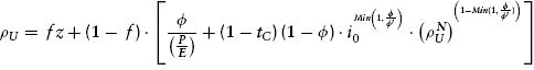
This last equation is our destination, and a highly useful result. In short, we can observe the leverage and P/E ratios from prevailing market prices. The effective tax rate is also observable. Consequently, inputting estimates for the capital spending reinvestment fraction f and the inflation-adjusted profitability z allows us to translate observed market prices into a basis for making expected return judgments. In the abstract, this replicates the results obtained in Chapters 4, 5, and 7.
EXTRACTING EXPECTED EQUITY RETURNS FROM OBSERVED PRICE/EARNINGS RATIOS: PART II
As noted in previous chapters, we are able to observe the interest rate on corporate debt at the same time we observe market common equity prices and P/E’s. However, in order to produce a set of expected return estimates over a wider set of scenarios, it is necessary to account for the fact that the interest rate on corporate debt will bear some relationship to the degree of corporate leverage, at least past some sufficiently low level of outstanding debt.
Borrowing from prior discussions, we are able to model the interest rate on corporate debt as the product of two terms, the first involving the core inflation rate and the second involving the real yield on corporate debt:
We further specify that the real yield on debt is a function of the degree of corporate leverage and is inversely related to the equity-to-capitalization ratio, that is:
The result of these specifications is that the nominal yield on corporate debt is also inversely related to the equity-to-capitalization ratio (or, alternatively, positively related to the debt ratio):
To facilitate tractable mathematics while still keeping with empirically observed results, we propose equation (9.15) for the yield on corporate debt:
where
Max(A,B) = the maximum value of the two terms “A” and “B”
i0 = nominal corporate debt yield for corporate debt with essentially zero default risk
exp(·) = the mathematical operator standing for exponentiation by the base of the natural logarithm “e” ≈ 2.71828
a = a scaling constant that is true across all values of the equity-to-capitalization ratio φ
φ′ = equity-to-capitalization ratio below which the corporate debt yield begins to rise above i0 due to the possibility of debt default
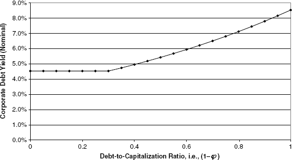
Figure 9.4 presents an application of equation (9.15) where the threshold debt ratio is 30%. The presumption is that a completely leveraged firm would have a corporate debt yield equal to the after-tax nominal equity discount firm for an unleveraged firm. This is consistent with the idea that at such an extreme case, the debt holders would be de facto equity owners of the whole firm. In actual practice, market debt-to-capitalization ratios, for nonfinancial companies outside of bankruptcy, are rarely observed above the 0.5 to 0.6 range, so the actual results in this range are difficult to envision and extrapolate. However, these assumptions regarding corporate debt yields serve as a reasonable approximation.
FIGURE 9.4 Corporate Debt Yield as a Function of Debt Leverage
The question that naturally arises is how to obtain the scaling constant to produce something like Figure 9.4. To answer, the first step is to streamline equation (9.15):
We have assumed that when φ = 0, the nominal corporate debt yield would equate to the nominal discount rate for the unleveraged firm, ![]() , as
, as
defined next.
Utilizing equation (9.16) and equation (9.17), where φ = 0 in the latter expression, we obtain the expression:
It is a simple matter to rearrange this equation to solve for the scaling constant a:
We encounter something of an obstacle in this expression, however. In attempting to extract values of both real and nominal unleveraged equity discount rates (ρU and ![]() ) from market P/E and leverage relationships, we are faced with the difficulty that we seemingly need to know in advance, for purposes of equation (9.19), that very thing that we are trying to infer.
) from market P/E and leverage relationships, we are faced with the difficulty that we seemingly need to know in advance, for purposes of equation (9.19), that very thing that we are trying to infer.
Fortunately, the problem is readily solvable with a combination of simple algebra and modest computational effort. Starting with the algebra, and assuming that we are dealing with circumstances where actual leverage exceeds the threshold level just defined (i.e., φ ≤ φ′), we are able to insert the applicable part of equation (9.16) into the fundamental relationship, equation (9.11). We do this while simultaneously making use of the formula for the scaling constant from equation (9.19). This produces:
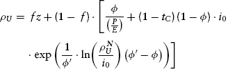
We make the first of a number of necessary algebraic and logarithmic rearrangements:
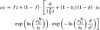
which can be simplified somewhat to get
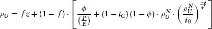
and, finally:
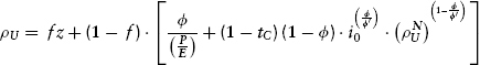
Equation (9.23) covers the case where leverage is in excess of the threshold value. To create a more general formulation, we can meld the above-threshold case of (9.23) with the below-threshold case of (9.11) to obtain:
The last step is to factor the nominal equity discount rate into its constituent parts on the right-hand side of (9.24). Doing so results in the generalized analog to equation (9.11):
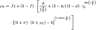
The good news is that we have a general formulation for converting P/Es into inflation-adjusted discount rates. The bad news is that formula (9.25) is algebraically intractable, which means that there is no straightforward way to get the real discount rate isolated and set equal to an expression that contains only the other variables. There is no need for discouragement, though, since a little bit of microchip computing power allows us to employ an iterative search algorithm (fancy talk for “trial and error” or “guess and check”).
This approach is set forth in Table 9.1. Beginning with iteration 1, we assume a reasonable value for the real discount rate ρU, insert it into the right-hand side (RHS) of equation (9.25) and, along with the other input variables, see what value is obtained for the left-hand side (LHS) of the equation. Then we use the value so obtained as the input value for the right-hand side of the equation and repeat the entire process.
TABLE 9.1 Schematic of Convergent Recursive Solution Method
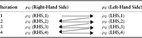
When the difference between the right-hand side and the left-hand side values is sufficiently small, the iteration process is terminated.
With reasonable initial seed values for the inflation-adjusted discount factor (i.e., 4% to 10%), the entire process acts as a rapidly converging mathematical attractor. The rapid rate of convergence is such that four iterations are usually more than sufficient to obtain accuracy of 1 basis point or better. Because of this rapid iteration, simple spreadsheets can be set up in Excel or Lotus 1-2-3; more complicated numerical programming in higher-level software languages is certainly possible but not necessary.
EXTRACTING EXPECTED EQUITY RETURNS FROM OBSERVED PRICE/EARNINGS RATIOS: PART III
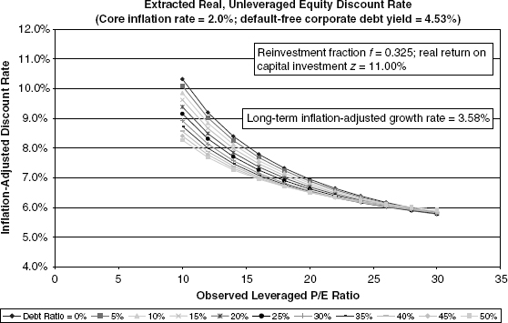
We are at last in a position to obtain and view results. Figures 9.5, 9.6, and 9.7 differ with regard to assumptions of capital reinvestment rates and the profitability of corporate capital spending. Since the emphasis in this section is primarily on broad common equity composites, the figures do not focus on growth rates substantially out of the norm for the economy in the aggregate.5
FIGURE 9.5 Case 1: Baseline Growth, Low Inflation
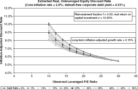
FIGURE 9.6 Case 2: Lower Growth, Low Inflation
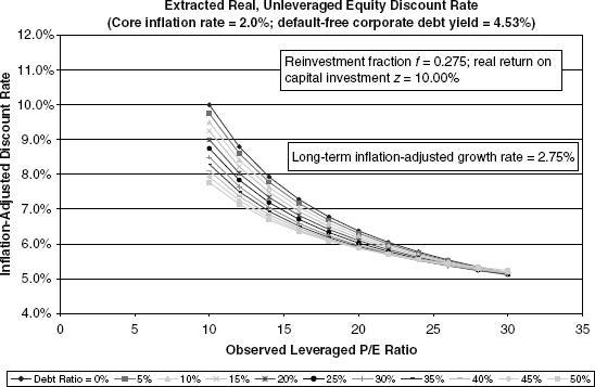
FIGURE 9.7 Case 3: Higher Growth, Low Inflation
In Figures 9.8 and 9.9, the underlying, inflation-adjusted growth and cash flow assumptions match those of Figure 9.5. The differences are that
FIGURE 9.8 Case 4: Baseline Growth, Medium Inflation
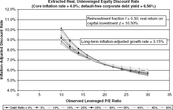
FIGURE 9.9 Case 5: Baseline Growth, High Inflation
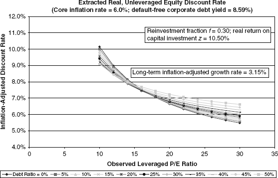
we examine core inflation rates of 4.0% and 6.0%, respectively. The interesting differences, versus the low-inflation case, are that the P/E ratios for more highly leveraged instances produce somewhat higher estimates of unleveraged, inflation-adjusted equity discount rates. The phenomenon is apparent at assumed leverage fractions that are well above what is seen in historical data and therefore warrant brief discussion.
We start by referring back to equation (9.6), which is presented again for convenience:
The model’s basic logic states that both the current period value of the unleveraged firm, VU, and the inflation-adjusted cash flow from current period operations, XU, are invariant over different core inflation rates. Since we are holding the debt ratio constant for purposes of this analysis, D = (1 − φ)VU is also constant. However, as the core inflation rate changes, the nominal corporate debt yield, i, must rise in accordance with equation (9.12). With an unchanging numerator and a declining denominator, the P/E ratio must necessarily move up.
What is happening in economic terms is that the higher nominal interest rate due to higher inflation must “front-end” the cash flow to debt holders to keep unchanged the debt holder net present value. Essentially, the higher coupon payment must offset the deterioration of future coupon and principal values owing to stepped-up inflation. Of course, this intertemporal shifting of cash flow and net present value works in reverse for equity holders. In other words, the declining inflation-adjusted value of cash payments to debt holders in future years means a higher growth rate in real cash flow to equity holders than would be the case in low-inflation scenarios. Hence, a higher P/E ratio results for any given observed initial period unleveraged corporate cash flow.
To some degree, this is a theoretical curiosity, since the debt ratios observed for the market composites are below 0.2 most of the time, thus reducing the impact on the denominator in equation (9.6). This is why Figures 9.8 and 9.9 show much less shifting in the curves for low levels of leverage. (Appendix I contains a more detailed explanation.)
CREATING EFFICIENT PORTFOLIOS: UNCONSTRAINED CASE
We define efficient portfolios as those portfolios having the minimum variance6 for their respective expected return targets. This set of efficient portfolios can be plotted against either variance or standard deviation, thus permitting investors to choose among this set of portfolios in accordance with their risk preferences and other institutional constraints. (The selection process is discussed in Chapter 10.)
This task of portfolio construction requires these input estimates: expected inflation-adjusted returns for each asset class, return variance for each asset class, and correlations between the returns of each asset class. Our work up to now has given us methods for establishing expected returns as well as variances for each of our asset classes. We still need a method for obtaining correlations. For the sake of exposition, however, we defer such derivations and proceed as if we had the correlations in hand. Throughout the rest of the book, we assume that the asset return processes are close enough to the normal distribution that mean/variance analysis is valid, since this is the presumed basis for investors’ selections among efficient portfolios.
We first create efficient portfolios for the typical case where there are no limitations on portfolio weights; this is commonly referred to as the unconstrained weights case. The discussion here, while sufficiently formal, centers on the treatment of three different asset classes: TIPS, fixed-rate debt, and a common equity composite. The presentation is also laid out in such a way that the reader can find solutions even with noncomplicated software, such as Excel or Lotus 1-2-3.
The mathematical formulation of the problem reflects these definitions:
wi = fraction of portfolio invested in asset class i
μi = expected return of asset class i
R = target expected portfolio return
σi = standard deviation of return for asset class i
ri,j = correlation of returns between asset classes i and j
σP = standard deviation of return for the entire portfolio
The formal system of equations represents the minimization of portfolio variance subject to the restrictions that the expected portfolio return equals the target and that the portfolio weights sum to unity (100%). In mathematical form:
The problem is solved by the method of LaGrange multipliers, in which we obtain n + 2 equations in the n + 2 variables (n portfolio weights w1, . . ., wn and the two LaGrange multipliers λ1 and λ2 that correspond to restrictions (9.27) and (9.28), respectively).
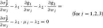
Two of the equations are the portfolio restriction equations (9.27) and (9.28). The remaining n equations are obtained via this partial differentiation process:
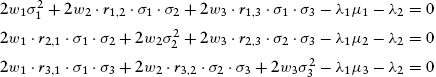
Since equations g1 and g2 are very simple mathematically, their partial derivatives transform equation (9.29) into:
With our three asset classes, it is easy and worthwhile to expand equation (9.30). The partial differentiation creates a series of linear equations that are easy to solve with basic matrix algorithms.
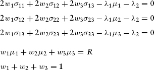
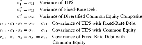
To cut down on some of the visual clutter, we can streamline notation by recollecting that ri,j = rj,i for all j ≠ i and that rj,j = ri,i = 1. This allows us to define:
These new sigmas with double subscripts are simply an expression of the term “covariance,” remembering that the covariance of a variable with itself is by definition that variable’s variance. With this reduction in clutter, we repeat system (9.31) in a somewhat more aesthetic manner. At the same time, we write out the accompanying investment restriction equations (9.27) and (9.28), thereby obtaining:
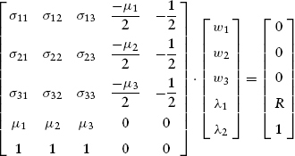
With modern spreadsheet software, it is simple enough to recast the system of equations from (9.33) into matrix form in order to take advantage of matrix multiplication and inversion functions. After dividing out all the 2s, the matrix formulation, from which the reader should see how to generalize to more than three asset classes, is:
The solution to the linear equation system (9.34) is obtained by first finding the inverse of the square matrix that contains the covariances, the individual asset returns, and the other constants of conservation. The inverted matrix is then multiplied by both sides, thus producing:
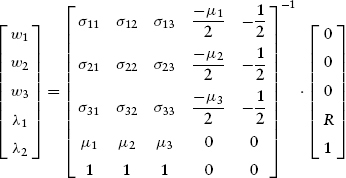
Inspection of equation system (9.35) shows that the portfolio weights will vary as the target expected return R is changed. In fact, since the inverted matrix is determined solely by the expected return and covariance structure of underlying asset classes, the underlying portfolio weights change in a linear fashion with respect to changes in target return R. When such changes in asset weights are translated into variance, or standard deviation, the relationship is the positively sloped and convex relationship as typified in Figure 9.10.
FIGURE 9.10 Example of Mean/Variance Efficient Portfolios
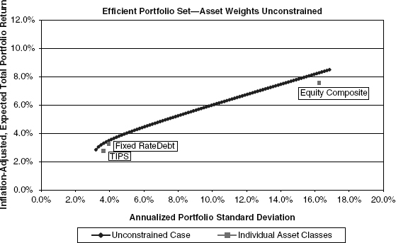
The figure also presents the returns and standard deviations for each of the underlying asset classes. As a result of the benefits of diversification, the set of efficient portfolios must necessarily lie to the left of and above each of the asset classes (Expressed differently, for any given target return corresponding to a particular asset class, a diversified portfolio can be formed to achieve the same expected return, but with lower standard deviation.) The complete set of efficient portfolios has a minimum attainable standard deviation. As the target expected return is raised, the standard deviation also rises in a manner consistent with an algebraic hyperbola.7
CREATING EFFICIENT PORTFOLIOS: CASE WHERE ASSET WEIGHTS ARE REQUIRED TO BE NONNEGATIVE
The traditional analysis of portfolio construction often stops at this point. However, as practitioners, we find more often the rule than the exception that portfolio weights for the various asset classes cannot be less than zero. That is, borrowing money and/or short selling is prohibited. Because of this fact, we are well advised to investigate portfolio construction under such constraints.
The mathematical statement of the problem starts out the same as equations (9.26) through (9.28), but adds these constraints:
or, in our particular case,
![]()
The nature of the inequality constraints introduces a complicated non-linearity into the problem. Consequently, the solution does not immediately boil down into a simple, easily programmable system of equations as shown in (9.33) and (9.34). In fact, problems of this nature must be solved by satisfying Kuhn-Tucker (KT) conditions, which are named after the authors who studied the problem in the 1950s.
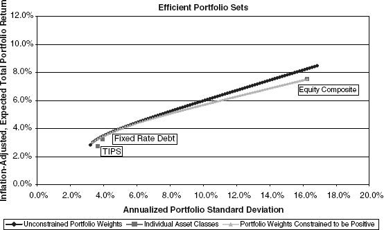
In our three-asset example, we set down first the equation system for solving the unconstrained case and then contrast it with the constrained case where the KT conditions are applied. (Readers with a less technical background are invited simply to review the results in Figure 9.11.)
FIGURE 9.11 Example of Efficient Portfolios Including Impact of Nonnegativity Constraints on Asset Weights
Unconstrained Weights System:
Constrained Weights System—Kuhn-Tucker Conditions:
Our difficulties can be relieved to some extent because, except for degenerate cases, the target return constraints and the portfolio conservation equations (i.e., the bracketed terms in equations (9.41) and (9.42)) must equal zero. Thus, the only tricky nonlinear equations will arise from condition (9.40). Utilizing information about portfolio weights from the solution of the Unconstrained Weights System, we can take instances where portfolio weights are less than zero and then treat them in system (9.40) as if they were zero, thus leaving us with two linear equations in two unknowns, thereby permitting us to solve the bracketed terms in equation (9.40) for such remaining two variables. Specifically, we would follow the method outlined for solving the three-variable, unconstrained case, but with a solution matrix reduced by the one row and the one column in order to omit the asset that was constrained to be zero.
If more than one variable must be constrained to zero, the system degenerates, and there are not enough variables in order to meet the constraints. With a small number of assets or asset classes, the programming of a solution is not unduly burdensome.
The best way to demonstrate the impact of a constrained portfolio is pictorially. Figure 9.11 compares the set of constrained portfolios with the set of unconstrained portfolios shown in Figure 9.10 and drawn to the same scale.
The requirement of nonnegative asset weights means that in many instances, both at high and very low levels of standard deviation, the unconstrained portfolio obtains better returns for any given degree of portfolio standard deviation (or risk). As can also be seen, where the nonnegativity constraints are not binding, the two curves overlap.
The divergence between the cases of constrained and unconstrained weights may be more or less than shown in Figure 9.11, depending on changes in relative expected returns and volatilities. We will see this in greater detail in Chapter 10.
COMPUTING THE VARIANCE/COVARIANCE MATRIX INPUTS
We have assumed to this point that we had the variance and covariance estimates in hand. We now backtrack to show how those inputs actually are obtained. We postponed this fairly technical discussion so as not to interrupt the overview of portfolio creation.
With three asset classes, we have to deal with three variance terms and three two-way covariances between the various asset classes. We define them accordingly, under two equivalent sets of notation already presented:
In Chapter 8, we dwelt at length on the formula for deriving the standard deviation for common equity. The approach was first to determine the volatility of the unleveraged value of the firm, V, and then to adjust for debt leverage in the corporate capital structure. Doing this involves first repeating equation (8.7)
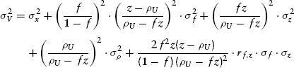
and then utilizing the full-blown debt leverage formula from equation (8.23):
or, alternatively, utilizing the debt leverage approximation method from equation (8.24)
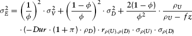
In connection with our derivation of equity volatility, we also developed a formula for the variance of fixed-rate debt. This was:
It is an easy step from this formula for fixed-rate debt return volatility to the formula for Treasury Inflation Protected Securities:
The TIPS formula omits the term attributable to changes in the core inflation rate, which is in line with our findings in Chapter 2. Thus, the volatility for TIPS returns is due strictly to its duration (which is not necessarily that of fixed-rate debt), to the current value of the inflation-adjusted discount rate, and to the variance of the inflation-adjusted discount rate (which is also not necessarily equal to that of fixed-rate debt).
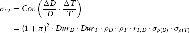
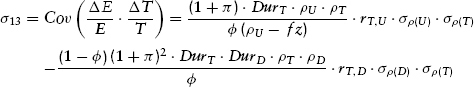
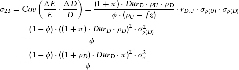
The covariance formulas are analogous to the variance expressions insofar as they reflect a mix of both (1) current market relationships (yields, discount rates, duration, etc.) and (2) presumably fundamentally stable econometric relationships (variances and covariances of inflation-adjusted discount rates and core inflation rates). Appendix K presents the derived covariance expressions among the various asset classes. They are reproduced here from equations (K.12), (K.13), and (K.14), respectively, with self-explanatory notational changes:
We explore some implications of these formulas in Chapter 10 after first deriving a method for selecting among efficient portfolios for the purpose of obtaining the portfolio most suitable to an investor with given risk preferences.
1 With a normal distribution, Probability(–1 ≤ Z ≤ 1) = Probability(Z ≤ 1) − Probability(Z ≤ −1) ≈ 84.5% − 15.9% = 68.3%.
2 With a normal distribution, Probability(-2 ≤ Z ≤ 2) = Probability(Z ≤ 2) − Probability(Z ≤ −2) ≈ 97.5% − 2.3% = 95.4%.
3 An introductory text on investing, such as Reilly’s Investments, provides a simple treatment of the difference between geometric and arithmetic average returns. The appropriateness of the expected arithmetic return as the basis for cash flow discounting is treated concisely by Ibbotson and Sinquefield in Chapter 9 of Stocks, Bonds, Bills, and Inflation: Historical Returns (1926–1987).
4 This step follows from our practitioners’ assumption from Chapter 4 that normal depreciation, depletion, and amortization (DDA) is roughly equal to the cash flow necessary for reinvestment to maintain “tangible” firm value.
5 For a refresher on the impact of near-term growth rates prevailing prior to an eventual, sustainable growth rate, the reader is referred back to Figure 3.8 in Chapter 3.
6 Or, alternatively, efficient portfolios can be defined as having the minimum standard deviation, that is, the square root of variance, for each target expected return.
7 In a hyperbola, the curvature ultimately gives way to a line that approaches a linear asymptote.