
Stability and Robust Stability of a Large-Scale NCS
Abstract
Stability and robust stability are essential for a system to work properly. In this chapter, we investigate verifications of these two important properties of a large-scale system. We mainly focus on computational complexity of a verification criterion. As in the previous chapters, the large-scale system under investigation is permitted to have subsystems with completely different dynamics and fixed but arbitrary subsystem connections. We derive some necessary and sufficient conditions that explicitly depend on the subsystem connection matrix. In addition, we also obtain conditions that essentially depend separately on parameter matrices of each individual subsystem and its out-degrees.
Keywords
large-scale system; linear matrix inequality; networked system; robust stability; stability
7.1 Introduction
To guarantee a satisfactory work of a system, it is necessary that its behavior can automatically return to its original trajectory after being perturbed by some external disturbances and/or when the system is not been originally set to the desirable states at the initial time instant. A system with this property is usually called stable. In other words, stability must be first guaranteed for a system to accomplish its expected tasks properly. In addition, as modeling errors are generally unavoidable, stability of a system must be kept even if some of its model parameters deviate from their nominal values and/or even if some other dynamics enter into the system behavior that are not included in its model. Due to the importance of these properties, verification of the stability and robust stability attracted extensive attentions for a long time in various fields, especially in the fields of systems and control [1]. Well-known results include Lyapunov stability theory, the Routh–Horwitz criterion for continuous-time systems, the Jury criterion for discrete-time systems, and so on. Although numerous milestone conclusions have been established, various important issues still require further investigations.
Especially, when a large-scale networked system is concerned, development of less conservative, more computationally efficient criteria is still theoretically challenging. Stimulated by the development of network and communication technologies and so on, renewed interests in this problem have extensively raised recently [2–4].
In [2], by means of introducing a spatial ![]() -transformation, some sufficient conditions have been derived, which are computationally attractive for the verification of the stability of spatially distributed systems. On the other hand, in [5], situations are clarified under which these conditions become also necessary for a spatially distributed system to be stable. Through adopting some parameter-dependent Lyapunov functions, in [6], a less conservative sufficient condition for this stability verification was derived. In addition, [7] reveals some important relations between the stability of a large-scale networked system and the structured singular value of a matrix. To apply these results, however, it is required that every subsystem has the same dynamics and that all subsystems are connected regularly and along some particular spatial directions. On the other hand, when a large-scale system has a so-called sequentially semiseparable structure, an iterative method is successfully developed in [8] for its stability verifications.
-transformation, some sufficient conditions have been derived, which are computationally attractive for the verification of the stability of spatially distributed systems. On the other hand, in [5], situations are clarified under which these conditions become also necessary for a spatially distributed system to be stable. Through adopting some parameter-dependent Lyapunov functions, in [6], a less conservative sufficient condition for this stability verification was derived. In addition, [7] reveals some important relations between the stability of a large-scale networked system and the structured singular value of a matrix. To apply these results, however, it is required that every subsystem has the same dynamics and that all subsystems are connected regularly and along some particular spatial directions. On the other hand, when a large-scale system has a so-called sequentially semiseparable structure, an iterative method is successfully developed in [8] for its stability verifications.
The concept of diagonal stability has also been utilized in the stability verification of a large-scale system. Particularly, stability of a networked system is investigated in [3] for systems consisting of only passive subsystems and having special structures. Influence of time delays on the stability of a large-scale system has been studied in [9] using a description of the so-called integral quadratic constraints. On the basis of the same descriptions for modeling errors, a sufficient condition is derived in [10] for the verification of the robust stability of the large-scale networked system described by Eqs. (6.1) and (6.2) with both its subsystem parameters and its subsystem connection matrix being time invariant. When modeling errors affect system input–output behaviors in a linear fractional way, some results are established in [11] on influence of subsystem interactions on the stability and robust stability of a networked system. Necessary and sufficient conditions are expressed there explicitly using the subsystem connection matrix of a networked system, and influence of the out-degree of a subsystem on the stability and robust stability of a networked system have also been clarified.
In this chapter, we summarize the results developed in [10,11] for the stability and robust stability of a large-scale NCS. Some necessary and sufficient conditions are given that explicitly take system structures into account, as well as some necessary or sufficient conditions that depend separately only on parameters of each subsystem and the subsystem connection matrix. Although the latter conditions are not necessary and sufficient, they can be verified independently for each individual subsystem and are therefore attractive for a large-scale NCS from the viewpoint of both numerical stability and computational costs. In addition, when the robust stability of an NCS is under investigation, both parametric modeling errors and unmodeled dynamics are permitted.
7.2 A Networked System With Discrete-Time Subsystems
In this section, we attack stability and robust stability of a networked system under the condition that each of its subsystem is described by a discrete-time model. Parallel results can be developed for a system with its subsystem dynamics described by a continuous-time model, that is, a set of first-order differential equations.
7.2.1 System Description
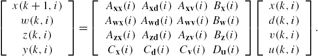
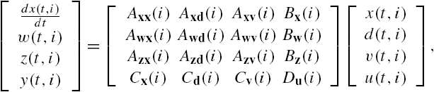
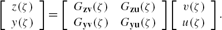
The NCS Σ investigated in this section is the same as that of the previous chapters, which has also been adopted in [10–12]. This system is constituted from N linear time-invariant dynamic subsystems, whereas the dynamics of its ith subsystem ![]() is described by the following state space model like representation:
is described by the following state space model like representation:

where ![]() . Moreover, its subsystems are connected through
. Moreover, its subsystems are connected through
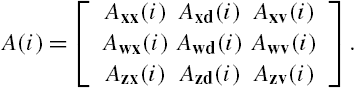
As in the previous chapters, here ![]() and
and ![]() are respectively defined as
are respectively defined as ![]() and
and ![]() . Moreover, k and i stand respectively for the temporal variable and the index number of a subsystem,
. Moreover, k and i stand respectively for the temporal variable and the index number of a subsystem, ![]() represents the state vector of the ith subsystem
represents the state vector of the ith subsystem ![]() at the time instant k,
at the time instant k, ![]() /
/![]() represent its output/input vector to/from other subsystems, and
represent its output/input vector to/from other subsystems, and ![]() and
and ![]() represent respectively its output and input vectors. Once again, as in the previous chapters, to distinguish
represent respectively its output and input vectors. Once again, as in the previous chapters, to distinguish ![]() and
and ![]() respectively from
respectively from ![]() and
and ![]() ,
, ![]() and
and ![]() are called internal output/input vectors, whereas
are called internal output/input vectors, whereas ![]() and
and ![]() are called external output/input vectors.
are called external output/input vectors.
Throughout this section, the dimensions of the vectors ![]() ,
, ![]() ,
, ![]() ,
, ![]() , and
, and ![]() , are assumed respectively to be
, are assumed respectively to be ![]() ,
, ![]() ,
, ![]() ,
, ![]() , and
, and ![]() . Moreover, we assume that every row of the matrix Φ has only one nonzero element, which is equal to one. As argued in the previous chapters, this assumption does not sacrifice any generality of the adopted system model. Note also that an approximate power-law degree distribution exists extensively in science and engineering systems, such as gene regulation networks, protein interaction networks, internet, electrical power systems, and so on. For these systems, interactions among subsystems are sparse, and the matrix Φ usually has a dimension significantly smaller than that of its state vector [10,12–14]. Under such a situation, results given in this section work well in general.
. Moreover, we assume that every row of the matrix Φ has only one nonzero element, which is equal to one. As argued in the previous chapters, this assumption does not sacrifice any generality of the adopted system model. Note also that an approximate power-law degree distribution exists extensively in science and engineering systems, such as gene regulation networks, protein interaction networks, internet, electrical power systems, and so on. For these systems, interactions among subsystems are sparse, and the matrix Φ usually has a dimension significantly smaller than that of its state vector [10,12–14]. Under such a situation, results given in this section work well in general.
7.2.2 Stability of a Networked System
To develop a computationally attractive criterion for the stability of system Σ and for its robust stability against both parametric modeling errors and unmodeled dynamics, the following results are at first introduced, which are well known in system theories [1,15–17].
Lemma 7.1
Concerning a discrete LTI system with its state space model being ![]() ,
, ![]() , it is stable if and only if
, it is stable if and only if ![]() .
.
Note that well-posedness is essential for a system to work properly. In fact, a plant that does not satisfy this requirement is usually hard to be controlled, and/or its states are in general difficult to be estimated [1,4,12]. It is therefore assumed in the following discussions that the networked system Σ under investigation is well-posed, which can be explicitly expressed as a requirement that the associated matrix is invertible.
When each its subsystem is linear and time-invariant and the subsystem connection matrix is also time invariant, the networked system Σ itself is also linear and time invariant. From Lemma 7.1 it is clear that the requirement that the networked system Σ is stable can be equivalently expressed as that all the eigenvalues of its state transition matrix are smaller than 1 in magnitude. To make mathematical derivations more concise, we first define the following matrices: ![]() ,
, ![]() ,
, ![]() , and
, and ![]() , where
, where ![]() , v or z. Moreover, denote
, v or z. Moreover, denote ![]() ,
, ![]() , and
, and ![]() respectively by
respectively by ![]() ,
, ![]() , and
, and ![]() . Then straightforward algebraic manipulations show that the well-posedness of the networked system Σ is equivalent to the regularity of the matrix
. Then straightforward algebraic manipulations show that the well-posedness of the networked system Σ is equivalent to the regularity of the matrix ![]() , that is, this matrix is invertible. Moreover, when the networked system Σ is well-posed, its dynamics can be equivalently described by the following state space model:
, that is, this matrix is invertible. Moreover, when the networked system Σ is well-posed, its dynamics can be equivalently described by the following state space model:

This expression gives a lumped state space model of the networked system Σ and is completely the same as that adopted in Lemma 7.1. This property can be understood more easily if we define the matrices A, B, C, and D respectively as

Clearly, all these matrices are time invariant. Moreover, the input–output relation of the networked system Σ has been rewritten completely in the same form as that in Lemma 7.1. As in the verification of controllability and observability of the networked system, this relation enables application of Lemma 7.1 to the stability and robust stability analysis of the networked system Σ. However, it is worth noting that a networked system usually has a great amount of subsystems, which means that the dimensions of the associated matrices in the lumped model are in general high. Hence, when a large-scale networked system is under investigation, it is usually not numerically feasible to straightforwardly apply the results of Lemma 7.1 to its analysis and synthesis. In addition, note that the inverse of the matrix ![]() is required in the aforementioned expressions, and this inversion is in general not numerically stable when the dimension of this matrix is high and/or when this matrix is nearly singular. These imply that calculations of the parameter matrices A, B, C, and D of the lumped model itself might not be reliable. As discussed in Chapter 3, these difficulties happen also to verifications of the controllability and/or the observability of the networked system Σ.
is required in the aforementioned expressions, and this inversion is in general not numerically stable when the dimension of this matrix is high and/or when this matrix is nearly singular. These imply that calculations of the parameter matrices A, B, C, and D of the lumped model itself might not be reliable. As discussed in Chapter 3, these difficulties happen also to verifications of the controllability and/or the observability of the networked system Σ.
To develop a computationally feasible and numerically reliable criterion for the stability of the networked system Σ, the following properties of the matrix A is first established.
Lemma 7.2
Assume that the networked system Σ is well-posed. Then, a complex number λ is not an eigenvalue of the matrix A if and only if ![]() . Here, the transfer function matrix
. Here, the transfer function matrix ![]() is defined as
is defined as ![]() .
.
Proof
When system Σ is well-posed, we have that ![]() , which is equivalent to
, which is equivalent to ![]() . From this inequality and the definition of the matrix A, direct algebraic manipulations show that for an arbitrary complex number λ,
. From this inequality and the definition of the matrix A, direct algebraic manipulations show that for an arbitrary complex number λ,
Hence ![]() can be equivalently expressed as
can be equivalently expressed as
Note that ![]() is of full normal rank. On the basis of the definition of the transfer function matrix
is of full normal rank. On the basis of the definition of the transfer function matrix ![]() , the following formal expression can be derived straightforwardly:
, the following formal expression can be derived straightforwardly:
Assume that ![]() . Then, we can declare from Eqs. (7.5) and (7.6) that
. Then, we can declare from Eqs. (7.5) and (7.6) that ![]() if and only if
if and only if ![]() .
.
Note that the dimension of the matrix ![]() is finite. We can claimed that its eigenvalues only take isolated values. Hence, if
is finite. We can claimed that its eigenvalues only take isolated values. Hence, if ![]() , then there always exists
, then there always exists ![]() such that, for each
such that, for each ![]() ,
, ![]() . Assume further that
. Assume further that ![]() . Then, by Eq. (7.4),
. Then, by Eq. (7.4),
Therefore, we can declare from Eq. (7.6) that
On the contrary, assume that ![]() . If
. If ![]() , then we can declare from Eq. (7.4) that there exist vectors α and β such that
, then we can declare from Eq. (7.4) that there exist vectors α and β such that ![]() and
and
From Eq. (7.9) it is clear that ![]() belongs to the image of the matrix
belongs to the image of the matrix ![]() . We can therefore declare from matrix theories [18] that even though
. We can therefore declare from matrix theories [18] that even though ![]() , the vector α can still be expressed as
, the vector α can still be expressed as ![]() , where
, where ![]() denotes the pseudo-inverse of a matrix. We can claim from this expression that
denotes the pseudo-inverse of a matrix. We can claim from this expression that ![]() .
.
Substituting the expression for α into Eq. (7.10), we have that
This further leads to
Hence from the definition of the transfer function matrix ![]() and consistencies between the inverse and the pseudo-inverse of a matrix we can declare that
and consistencies between the inverse and the pseudo-inverse of a matrix we can declare that ![]() . This is a contradiction with the assumption. We can therefore claim that
. This is a contradiction with the assumption. We can therefore claim that ![]() . This completes the proof. □
. This completes the proof. □
On the basis of Eq. (7.5), it can be shown that the networked system Σ is stable, only when all the unstable modes of each of its subsystems are both controllable and observable. This conclusion can be established through a similarity transformation that divide the state space of each subsystem into a stable subspace and an unstable subspace, utilizing the relation of the following Eq. (7.11).
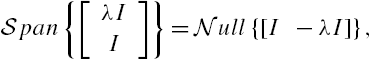
From Lemmas 7.1 and 7.2 it is clear that a necessary and sufficient condition for the networked system Σ to be stable is that, for every complex number λ satisfying ![]() , the matrix
, the matrix ![]() is regular. However, it is worth noting that when the networked system under investigation is constructed from a large amount of subsystems, although the subsystem connection matrix Φ is usually sparse, its dimension is still usually high. Moreover, the associated inequality must be checked for each complex number λ satisfying
is regular. However, it is worth noting that when the networked system under investigation is constructed from a large amount of subsystems, although the subsystem connection matrix Φ is usually sparse, its dimension is still usually high. Moreover, the associated inequality must be checked for each complex number λ satisfying ![]() . This is generally impossible through straightforward computations. By these observations it is safe to declare that some further efforts are still required to make the results of Lemma 7.2 applicable to a large-scale networked system.
. This is generally impossible through straightforward computations. By these observations it is safe to declare that some further efforts are still required to make the results of Lemma 7.2 applicable to a large-scale networked system.
To achieve these objectives, we recall the following property for the subsystem connection matrix Φ stated and proven in Chapter 3.
Let ![]() stand for the number of subsystems that is directly affected by the ith element of the vector
stand for the number of subsystems that is directly affected by the ith element of the vector ![]() ,
, ![]() . Define the matrices
. Define the matrices ![]() ,
, ![]() , and Θ respectively as
, and Θ respectively as ![]() and
and ![]() . It has been proven in [11] and Chapter 3 that
. It has been proven in [11] and Chapter 3 that

On the basis of these results, we derive a necessary and sufficient condition for the stability of the networked system Σ, which explicitly takes the structure of the networked system into account and is computationally attractive.
Theorem 7.1
Proof
Note that ![]() is equivalent to
is equivalent to ![]() . Moreover,
. Moreover,
and ![]() is equivalent to
is equivalent to
On the other hand, straightforward matrix operations show that
which implies that, for each fixed λ, a vector, say α, that can be expressed as

where ξ is a complex vector with a compatible dimension, belongs to the null space of the matrix ![]() . In other words, when the Laplacian variable λ is prescribed to a particular value, we have the following relation:
. In other words, when the Laplacian variable λ is prescribed to a particular value, we have the following relation:

In addition, note also that
which can be directly proven from Definitions 2.5 and 2.6.
On the basis of these relations, similar arguments as those in the proof of Theorems 1 and 3 of [19] and those in [5,10] show that ![]() ,
, ![]() , can be equivalently expressed as the existence of a positive definite matrix P such that
, can be equivalently expressed as the existence of a positive definite matrix P such that

On the other hand, direct algebraic manipulations show that

The proof can now be completed by substituting Eqs. (7.14) and (7.15) into Eq. (7.13). □
Compared with the available results, such as those of [2,3,6,7], an attractive characteristic of Theorem 7.1 is that there exist no restrictions on the model of the networked system Σ and the condition is both necessary and sufficient. On the other hand, note that the left-hand side of Eq. (7.12) depends linearly on the matrix P and that the structure of the networked system Θ, which is represented by the subsystem connection matrix Φ, is explicitly included in this equation. For a small size problem, feasibility of this matrix inequality can in general be easily verified using available linear matrix inequality (LMI) solvers. On the other hand, note that all the matrices ![]() with ⁎,
with ⁎, ![]() = x, z are block diagonal and a networked system usually has a sparse structure, which is reflected by the subsystem connection matrix Φ. In addition, efficient methods have been developed for sparse semidefinite programming, such as those in [10,20,21]. It is expected that the above condition works well also for a moderate size problem. This expectation has been confirmed through some numerical simulations reported in [11].
= x, z are block diagonal and a networked system usually has a sparse structure, which is reflected by the subsystem connection matrix Φ. In addition, efficient methods have been developed for sparse semidefinite programming, such as those in [10,20,21]. It is expected that the above condition works well also for a moderate size problem. This expectation has been confirmed through some numerical simulations reported in [11].
From its proof it is clear that although the matrices ![]() with
with ![]() , v, or z are block diagonal, the matrix P is usually dense. In addition, when the square of the matrix Θ in inequality (7.12) is replaced by
, v, or z are block diagonal, the matrix P is usually dense. In addition, when the square of the matrix Θ in inequality (7.12) is replaced by ![]() , the results of Theorem 7.1 become valid for an arbitrary subsystem connection matrix Φ. On the other hand, a necessary condition for the feasibility of this inequality obviously is
, the results of Theorem 7.1 become valid for an arbitrary subsystem connection matrix Φ. On the other hand, a necessary condition for the feasibility of this inequality obviously is
which can be proved to be equivalent to the existence of positive definite matrices ![]() for
for ![]() such that
such that
The last inequality can be verified for each subsystem independently.
It is worth pointing out that from Lyapunov stability theory we can directly declare that system Σ is stable if and only if there exists a positive definite matrix P such that ![]() , which is also a linear matrix inequality. However, as argued in [10,12] and the previous chapters, although the subsystem connection matrix Φ is generally sparse, the state transition matrix A is usually dense. This implies that computational complexity for feasibility verification of this equation is usually significantly greater than that of inequality (7.12), especially when the plant consists of a large amount of subsystems. Similar observations have also been reported in [10] for robust stability verification of system Σ with IQC described uncertainties.
, which is also a linear matrix inequality. However, as argued in [10,12] and the previous chapters, although the subsystem connection matrix Φ is generally sparse, the state transition matrix A is usually dense. This implies that computational complexity for feasibility verification of this equation is usually significantly greater than that of inequality (7.12), especially when the plant consists of a large amount of subsystems. Similar observations have also been reported in [10] for robust stability verification of system Σ with IQC described uncertainties.
When a system is of a very large-scale, numerical difficulties may still arise in verifying the condition of Theorem 7.1. To overcome these difficulties, one possibility is to find some matrices ![]() with
with ![]() and
and ![]() that have dimensions and partitions compatible with the matrix
that have dimensions and partitions compatible with the matrix ![]() such that
such that
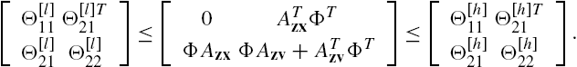
With availability of these matrices, direct algebraic operations show that a necessary condition for the stability of system Σ is the existence of a PDM ![]() for each
for each ![]() such that
such that

Moreover, when the superscript l is replaced by h, these inequalities become a sufficient condition. Clearly, these inequalities depend linearly on ![]() , and their dimensions are completely and independently determined by each individual system. These properties make them much more computationally attractive than Eq. (7.12). However, further efforts are required to find the matrices
, and their dimensions are completely and independently determined by each individual system. These properties make them much more computationally attractive than Eq. (7.12). However, further efforts are required to find the matrices ![]() in Eq. (7.16) with
in Eq. (7.16) with ![]() ,
, ![]() , and
, and ![]() such that the associated inequalities are both tight and computationally attractive.
such that the associated inequalities are both tight and computationally attractive.
Based on the properties of the SCM Φ, another computationally attractive sufficient condition is derived for the stability of system Σ.
Theorem 7.2
Denote the TFM ![]() by
by ![]() and assume that
and assume that ![]() <1 for each subsystem. Then system Σ is stable.
<1 for each subsystem. Then system Σ is stable.
Proof
From the definitions of the TFMs ![]() and
and ![]() it is obvious that
it is obvious that ![]() . Based on this relation and Eq. (7.11), we can directly prove that
. Based on this relation and Eq. (7.11), we can directly prove that

From the definition of the ![]() norm of a TFM we can declare that if
norm of a TFM we can declare that if ![]() , then
, then ![]() for
for ![]() . Note that
. Note that ![]() for every square matrix [18]. We can therefore further claim that when
for every square matrix [18]. We can therefore further claim that when ![]() and
and ![]() ,
, ![]() , it is certain that
, it is certain that
and hence ![]() . This completes the proof. □
. This completes the proof. □
Note that ![]() is completely determined by the SCM Φ and the parameters of the ith subsystem, and efficient methods exist for computing an upper bound of the
is completely determined by the SCM Φ and the parameters of the ith subsystem, and efficient methods exist for computing an upper bound of the ![]() norm of a TFM. Therefore, the condition of Theorem 7.2 can be easily verified, and its computational complexity increases only linearly with the increment of the subsystem number N. This means that for a large-scale networked system, the computation cost of Theorem 7.2 is in general significantly lower than that of Theorem 7.1. However, it is worth emphasizing that this condition is only sufficient and its conservativeness is still not clear. On the other hand, the numerical simulation results reported in [11] show that with the increment of the subsystem number and/or the magnitude of the subsystem matrix elements, conservativeness of Theorem 7.2 usually increases.
norm of a TFM. Therefore, the condition of Theorem 7.2 can be easily verified, and its computational complexity increases only linearly with the increment of the subsystem number N. This means that for a large-scale networked system, the computation cost of Theorem 7.2 is in general significantly lower than that of Theorem 7.1. However, it is worth emphasizing that this condition is only sufficient and its conservativeness is still not clear. On the other hand, the numerical simulation results reported in [11] show that with the increment of the subsystem number and/or the magnitude of the subsystem matrix elements, conservativeness of Theorem 7.2 usually increases.
Note also that the finiteness of ![]() implies the stability of the subsystem
implies the stability of the subsystem ![]() . Moreover, from the definition of the TFM
. Moreover, from the definition of the TFM ![]() norm we can see that
norm we can see that ![]() decreases monotonically with the decrement of any diagonal element of the matrix
decreases monotonically with the decrement of any diagonal element of the matrix ![]() . Theorem 7.2 therefore also makes it clear that for an NS consisting of stable subsystems, sparse connections are helpful in maintaining its stability, and subsystem interaction reduction can make an unstable system stable.
. Theorem 7.2 therefore also makes it clear that for an NS consisting of stable subsystems, sparse connections are helpful in maintaining its stability, and subsystem interaction reduction can make an unstable system stable.
On the basis of the results given in [19], here we provide a linear matrix inequality-based condition for the verification of the ![]() norm-based condition.
norm-based condition.
Note that ![]() is equivalent to
is equivalent to
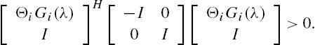
It can be directly proved from the structure of ![]() that the condition of Theorem 7.2 can be equivalently expressed as the following matrix inequality:
that the condition of Theorem 7.2 can be equivalently expressed as the following matrix inequality:

for every complex number λ such that ![]() .
.
Recall that ![]() is equivalent to
is equivalent to
Based on the definition of the ![]() norm of a transfer function matrix and Theorems 1 and 3 of [19], we can directly claim that
norm of a transfer function matrix and Theorems 1 and 3 of [19], we can directly claim that ![]() is equivalent to the existence of a positive definite matrix
is equivalent to the existence of a positive definite matrix ![]() such that
such that

which can be reexpressed as

Clearly, the left-hand side of this matrix inequality depends linearly on the matrix ![]() , and its dimension is completely determined by that of the ith subsystem
, and its dimension is completely determined by that of the ith subsystem ![]() . Therefore, feasibility of this inequality can be effectively verified in general.
. Therefore, feasibility of this inequality can be effectively verified in general.
Note that a necessary condition for the feasibility of inequality (7.22) is the existence of a positive definite matrix ![]() such that
such that
This inequality further leads to
According to the Lyapunov stability theory [1,2,4], this means that the matrix ![]() is stable. In other words, a necessary condition for the feasibility of inequality (7.22) is that when every subsystem of system Σ is completely isolated from interactions with all the other subsystems of the plant, then all they are stable. Clearly, this is generally not required to guarantee the stability of the whole system, noting that a controllable and observable open loop unstable system can be stabilized by an appropriately designed feedback controller. From these aspects it is also clear that the associated condition is generally conservative.
is stable. In other words, a necessary condition for the feasibility of inequality (7.22) is that when every subsystem of system Σ is completely isolated from interactions with all the other subsystems of the plant, then all they are stable. Clearly, this is generally not required to guarantee the stability of the whole system, noting that a controllable and observable open loop unstable system can be stabilized by an appropriately designed feedback controller. From these aspects it is also clear that the associated condition is generally conservative.
7.2.3 Robust Stability of a Networked System
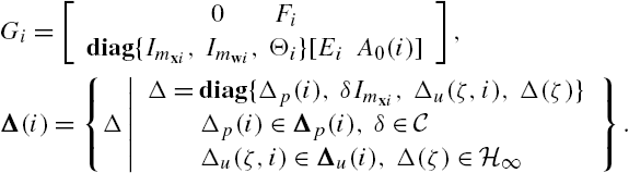
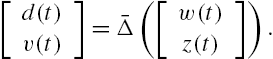
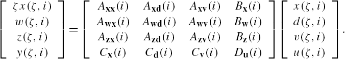
Modeling errors are unavoidable in practical engineering. A general requirement about a system property is that it is not sensitive to modeling errors, which is widely known as robustness of this property. This section investigates the robust stability of a networked system when there exist both parametric modeling errors and unmodeled dynamics in a state space model of each of its subsystems. To deal with this problem, an extra input vector and an extra output vector are introduced into the description of the dynamics of its ith subsystem ![]() with the purpose of reflecting influences of modeling errors while the subsystem connections remain unchanged. More precisely, the state space model of Eq. (7.1) is modified into the following form:
with the purpose of reflecting influences of modeling errors while the subsystem connections remain unchanged. More precisely, the state space model of Eq. (7.1) is modified into the following form:
In addition, the unmodeled dynamics in this subsystem and the parametric errors in the matrices ![]() with
with ![]() are respectively described by
are respectively described by
Here q stands for the one-step forward shift operator, ![]() and
and ![]() have respectively a prescribed structure represented by
have respectively a prescribed structure represented by ![]() and
and ![]() . Moreover,
. Moreover, ![]() and
and ![]() are known matrices with compatible dimensions. In this description, the matrices
are known matrices with compatible dimensions. In this description, the matrices ![]() and
and ![]() are introduced to reflect how parametric errors influence subsystem parameters, whereas
are introduced to reflect how parametric errors influence subsystem parameters, whereas ![]() and
and ![]() denote respectively unmodeled dynamics and parametric errors existing in the state space model. This description is general enough to describe a large class of system dynamics. Moreover, a widely adopted structure for modeling errors is that they are block diagonal [1,22].
denote respectively unmodeled dynamics and parametric errors existing in the state space model. This description is general enough to describe a large class of system dynamics. Moreover, a widely adopted structure for modeling errors is that they are block diagonal [1,22].
With this uncertainty model, the following results are obtained for the robust stability of the networked system Σ. Their proof is given in the appendix attached to this chapter.
Theorem 7.3
Note that the condition of Theorem 7.3 can be verified independently for each subsystem. This means that the well-developed SSV analysis methods can be directly applied to its verification in general. Compared with the results of [10], Theorem 7.3 is valid for a wider class of uncertainty models and have a lower computational complexity. As a matter of fact, its computational complexity increases only linearly with the increment of the subsystem number N.
On the other hand, from Eq. (7.A.4) we can derive another SSV-based sufficient condition for the robust stability of system Σ simultaneously using all subsystem parameter matrices and the subsystem connection matrix. However, the corresponding matrix and the uncertainty structure generally have a high dimension, which is not appropriate to be applied to a large-scale networked system.
7.3 A Networked System With Continuous-Time Subsystems
In this section, we investigate the robust stability of a networked system when its subsystem is described by a set of first-order differential equations and its modeling errors are described by several IQCs, which stand for integral quadratic constraint, and is to some extent a little abstract description. As in the previous section, similar arguments can lead to parallel results for am NCS with discrete-time subsystems.
7.3.1 Modeling Errors Described by IQCs
In the description of modeling errors, a well-known but relatively abstract expression is the so-called integral quadratic constraints (IQCs) [23,24]. As its name indicates, in this description, both integration and a quadratic form are utilized. More precisely, let ![]() be a bounded self-adjoint operator, and let
be a bounded self-adjoint operator, and let ![]() be a bounded and causal operator that maps a p-dimensional signal to a q-dimensional signal. If for each p-dimensional signal
be a bounded and causal operator that maps a p-dimensional signal to a q-dimensional signal. If for each p-dimensional signal ![]() with finite energy, that is,
with finite energy, that is, ![]() ,
,

then we say that the operator ![]() satisfies the IQC defined by the operator
satisfies the IQC defined by the operator ![]() , which is usually denoted by
, which is usually denoted by ![]() . This inequality is capable of describing many modeling errors adopted in system analysis and synthesis. For example, a
. This inequality is capable of describing many modeling errors adopted in system analysis and synthesis. For example, a ![]() -dimensional parametric modeling error Δ with
-dimensional parametric modeling error Δ with ![]() can be easily seen to satisfy
can be easily seen to satisfy

whereas the ![]() -dimensional unmodeled dynamics
-dimensional unmodeled dynamics ![]() with
with ![]() can be straightforwardly proved to meet the IQC
can be straightforwardly proved to meet the IQC

In addition to these, IQCs are also able to describe system properties like passivity, and combine several IQCs into a single IQC [25,26].
Utilization of IQCs in system analysis and synthesis can be traced back to the 1960s, in which they are extensively applied to the absolute stability analysis of a nonlinear system, whereas their applications to the analysis and synthesis of a system with modeling errors were started around the beginning of the 1990s [23–26]. A particularly important property of IQCs is that they have a clear frequency domain interpretation, which makes engineering intuition in system analysis and synthesis much clearer and easier to be understood. In particular, if the operator ![]() of Eq. (7.27) is linear and time invariant and has a transfer function matrix representation, then the IQC of Eq. (7.27) can be equivalently rewritten as
of Eq. (7.27) is linear and time invariant and has a transfer function matrix representation, then the IQC of Eq. (7.27) can be equivalently rewritten as

In addition to this, an IQC constraint is also capable of describing nonlinear dynamic uncertainties, which makes the associated system analysis and synthesis methods able to cope with nonlinear modeling errors.
The following results are fundamental in robust stability analysis of a system with IQC described uncertainties [10,25]. They also play central roles in the derivations of a criterion for the robust stability of a networked system, which is the main objective of this section.
Lemma 7.3
Consider a feedback system with ![]() and
and ![]() , where
, where ![]() and
and ![]() . Moreover, let
. Moreover, let ![]() be a bounded and self-adjoint operator. Suppose that
be a bounded and self-adjoint operator. Suppose that
- • for each
 , the feedback system with
  replaced by
 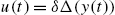 is well-posed;
 - •
 for arbitrary ;
 - • there exists a positive number ε such that for an arbitrary angular frequency
 , the following inequality is satisfied:

Then, the feedback system is robustly stable with respect to the uncertain operator ![]() .
.
Remark 7.1
For a particular uncertain operator ![]() , there may exist various bounded and self-adjoint operators
, there may exist various bounded and self-adjoint operators ![]() such that
such that ![]() . This is a well-encountered case in actual system analysis and synthesis [23]. Under such a situation, Lemma 7.3 declares that among these bounded and self-adjoint operators
. This is a well-encountered case in actual system analysis and synthesis [23]. Under such a situation, Lemma 7.3 declares that among these bounded and self-adjoint operators ![]() , if one of them satisfies inequality (7.29), then the feedback system consisting of
, if one of them satisfies inequality (7.29), then the feedback system consisting of ![]() and
and ![]() is robustly stable. Note that the conditions of Lemma 7.3 are only sufficient. An appropriate selection of this bounded self-adjoint operator
is robustly stable. Note that the conditions of Lemma 7.3 are only sufficient. An appropriate selection of this bounded self-adjoint operator ![]() is important in the reduction of the conservativeness of these conditions.
is important in the reduction of the conservativeness of these conditions.
7.3.2 Robust Stability With IQC-Described Modeling Errors
In this section, we investigate once again the robust stability of a networked system with dynamics described similarly as in Eqs. (7.23) and modeling errors for each subsystem described by an IQC. Rather than a discrete-time system, a continuous-time system is dealt with, that is, interactions among its subsystems are still described by an equation similar to Eq. (7.2), and the input–output relation of its ith subsystem by an equation similar to Eq. (7.23) with the signal transfer from ![]() to
to ![]() described by
described by
Moreover, there exists a bounded self-adjoint operator ![]() , such that
, such that ![]() . To avoid awkward presentations, we assume that there are no longer any other modeling uncertainties in the subsystem matrices
. To avoid awkward presentations, we assume that there are no longer any other modeling uncertainties in the subsystem matrices ![]() with
with ![]() .
.
More precisely, the dynamics of the ith subsystem ![]() is described by
is described by
whereas the subsystem interactions are described by
where the vectors ![]() and
and ![]() are defined similarly to the vectors
are defined similarly to the vectors ![]() and
and ![]() of Eq. (7.2), which are stacked respectively by the internal input vectors
of Eq. (7.2), which are stacked respectively by the internal input vectors ![]() and the internal output vectors
and the internal output vectors ![]() row by row.
row by row.
When the modeling errors in each subsystem of the networked system are described by Eq. (7.30), define the operators ![]() and
and ![]() as
as
where ![]() . Moreover, denote the vector
. Moreover, denote the vector ![]() by
by ![]() . Then it is clear from these definitions that
. Then it is clear from these definitions that
Note that

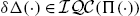
It is clear that if the modeling errors of each subsystem can be described by an IQC, then the total modeling errors of the whole networked system can also be described by an IQC. More precisely, we can straightforwardly prove from the definition of an integral quadratic constraint that the operator ![]() belongs to the set
belongs to the set ![]() if and only if for each
if and only if for each ![]() , the uncertainty operator
, the uncertainty operator ![]() of the subsystem
of the subsystem ![]() belongs to the set
belongs to the set ![]() . The proof is quite obvious and is therefore omitted.
. The proof is quite obvious and is therefore omitted.
The above relations can be expressed in a more explicit and concise way if the IQC associated inequality is described in the frequency domain for the modeling errors of each subsystem. More precisely, assume that for the ith subsystem ![]() , its modeling error
, its modeling error ![]() is described by
is described by
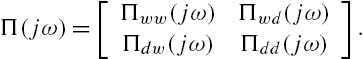
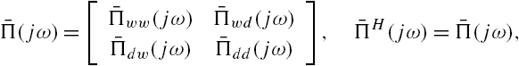
where ![]() is a complex matrix-valued function that is Hermitian at each angular frequency ω. Partition this matrix-valued function as
is a complex matrix-valued function that is Hermitian at each angular frequency ω. Partition this matrix-valued function as
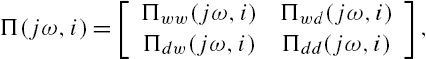
where ![]() is an
is an ![]() -dimensional complex matrix-valued function. Here
-dimensional complex matrix-valued function. Here ![]() . Using these functions, define the complex matrix-valued functions
. Using these functions, define the complex matrix-valued functions ![]() for
for ![]() . Moreover, on the basis of these complex matrix-valued functions, define the other complex matrix-valued function
. Moreover, on the basis of these complex matrix-valued functions, define the other complex matrix-valued function
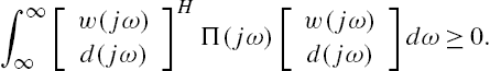
Then it is obvious that this complex matrix-valued function is Hermitian. In addition, for signals ![]() and
and ![]() defined by Eq. (7.34), straightforward algebraic manipulations show that
defined by Eq. (7.34), straightforward algebraic manipulations show that
In this section, we discuss only situations where each operator ![]() is time invariant. The temporal variable t is therefore omitted to have a concise expression in the following investigations.
is time invariant. The temporal variable t is therefore omitted to have a concise expression in the following investigations.
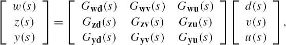
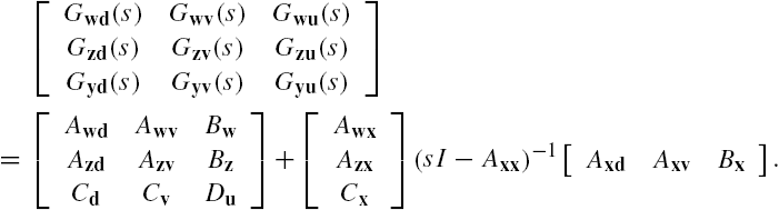
As in the previous section, the Laplace transform of a time series is denoted by the same symbol with temporal variable t replaced by s, the variable of the Laplace transform. Taking the Laplace transformation on both sides of Eqs. (7.31) and (7.32), we have that

Substitute the expression for the vector ![]() given by Eq. (7.41) into Eq. (7.40). Straightforward algebraic manipulations show that
given by Eq. (7.41) into Eq. (7.40). Straightforward algebraic manipulations show that

where
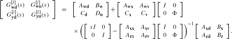
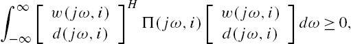
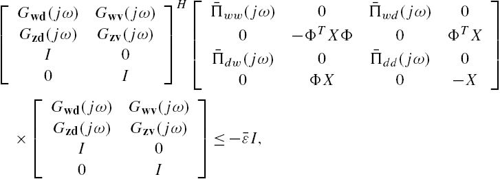
Clearly, when the dynamics of the networked system Σ are described by Eqs. (7.34) and (7.42), connections between its nominal system and modeling errors are completely the same as in Lemma 7.3. This implies that the results of this lemma may be straightforwardly applicable to the aforementioned networked system. More precisely, by Lemma 7.3 we have that when the modeling errors are described by Eq. (7.30) for each subsystem of the networked system described by Eqs. (7.23) and (7.32), there exists a Hermitian complex matrix-valued function ![]() satisfying
satisfying
at each angular frequency ω, and then this networked system is robustly stable against these modeling errors.
However, it is worth mentioning that, completely as the difficulties encountered in dealing with other issues related to a networked system with a large number of subsystems, such as controllability and/or observability verifications, and so on, the dimension of the transfer function matrix ![]() is generally high when the amount of subsystems is large. In addition to this, note that the inverse of a sparse matrix is in general dense. This means that in spite that the matrices
is generally high when the amount of subsystems is large. In addition to this, note that the inverse of a sparse matrix is in general dense. This means that in spite that the matrices ![]() with
with ![]() are block diagonal, both matrices
are block diagonal, both matrices ![]() and
and ![]() are also block diagonal, and that the subsystem connection matrix Φ is usually sparse, the transfer function matrix
are also block diagonal, and that the subsystem connection matrix Φ is usually sparse, the transfer function matrix ![]() is usually dense. Hence, for a large-scale networked system, direct applications of Lemma 7.3 may suffer from both computational cost and numerical stability problems.
is usually dense. Hence, for a large-scale networked system, direct applications of Lemma 7.3 may suffer from both computational cost and numerical stability problems.
To overcome these problems, the structure of the networked system is utilized in this section in its robust stability analysis, which has also been performed in the previous section when the modeling errors are described by Eqs. (7.24)–(7.26). For this purpose, the influences among the subsystems of the networked system, which is given by Eq. (7.2), is first expressed equivalently as an IQC.
Note that Eq. (7.2) is equivalent to that, for an arbitrary positive definite matrix X with an appropriate dimension, the following inequality is satisfied:
Hence, the subsystem interactions can be equivalently expressed as
Define the operator ![]() as
as

Then, obviously from the definitions of the associated vectors we have the equality
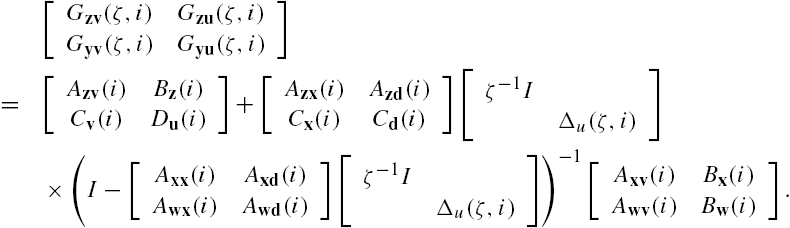
On the other hand, similarly to the derivation of Eq. (7.42), we can straightforwardly prove from Eq. (7.40) that
where
Differently from the transfer function matrices ![]() with
with ![]() and
and ![]() , which are defined in Eq. (7.42) and are usually dense, all the transfer function matrices
, which are defined in Eq. (7.42) and are usually dense, all the transfer function matrices ![]() with
with ![]() and
and ![]() are block diagonal.
are block diagonal.
Note that when ![]() , δΦ does not satisfy the IQC (7.44). This means that although Eqs. (7.46) and (7.47) construct a feedback connection as that of Lemma 7.3, its results cannot be directly applied to the verification of the robust stability of the networked system since its second condition is not satisfied. However, due to the specific structure of the transfer function matrix
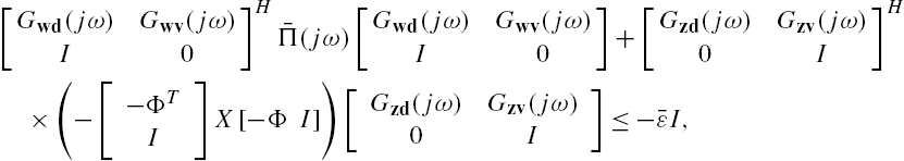
, δΦ does not satisfy the IQC (7.44). This means that although Eqs. (7.46) and (7.47) construct a feedback connection as that of Lemma 7.3, its results cannot be directly applied to the verification of the robust stability of the networked system since its second condition is not satisfied. However, due to the specific structure of the transfer function matrix ![]() , we can prove that satisfaction of the associated condition is equivalent to the feasibility of the matrix inequality of Eq. (7.43). As a matter of fact, we have the following results with their proof deferred to the appendix attached to this chapter.
, we can prove that satisfaction of the associated condition is equivalent to the feasibility of the matrix inequality of Eq. (7.43). As a matter of fact, we have the following results with their proof deferred to the appendix attached to this chapter.
Theorem 7.4
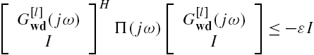
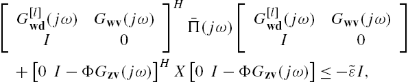
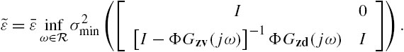
There exists a complex matrix-valued Hermitian function ![]() satisfying Eq. (7.43) if and only if there exist a complex matrix-valued function
satisfying Eq. (7.43) if and only if there exist a complex matrix-valued function ![]() , a positive scalar x, and a positive scalar
, a positive scalar x, and a positive scalar ![]() such that
such that
and for each ![]() with
with ![]() , we have the matrix inequality
, we have the matrix inequality
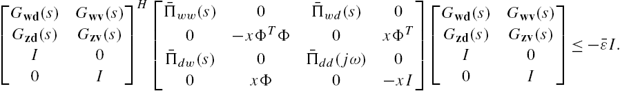
Compared to Eq. (7.43), all the transfer function matrices in Eq. (7.49) are block diagonal. In addition, the subsystem connection matrix Φ is generally sparse for a large-scale networked system. This makes it possible to use results about sparse matrix computations in the feasibility verification of the associated matrix inequality, for which many efficient algorithms have been developed [21,27]. Numerical studies in [10] show that it really can significantly reduce computation costs for various types of large-scale networked systems.
7.4 Concluding Remarks
In summary, this chapter investigates both stability and robust stability for a networked system with nominal LTI subsystems and time-independent subsystem connections. The plant subsystems can have different nominal TFMs, and there do not exist any restrictions on their interactions. Some sufficient and necessary conditions have been derived. These conditions only depend on the subsystem connection matrix and parameter matrices of each plant subsystem, which make their verification easily implementable in general for a large-scale networked system. However, under some situations, for example, when plant subsystems are densely interconnected, both the subsystem connection matrix Φ and some of the transfer function matrices ![]() may have a high dimension. In this case, results of this chapter usually do not significantly reduce computation costs, and further efforts are required to develop computationally more efficient methods.
may have a high dimension. In this case, results of this chapter usually do not significantly reduce computation costs, and further efforts are required to develop computationally more efficient methods.
In addition to these, influence of many important factors on the stability and robust stability of a networked system, such as signal transmission delays between subsystems, data droppings, and so on, have not been explicitly discussed here. Some of these factors, however, can be incorporated into a system model as modeling uncertainties [22,23], which may enable application of the results in this chapter to these situations.
7.5 Bibliographic Notes
Results of this chapter are on the basis of [10] and [11]. There are also various other researches on the stability and robust stability of a networked system, where its model has some special constraints, and different concepts of stability are utilized. For example, diagonal stability is investigated for a networked system in [3] with a cactus graph structure, which is basically based on system passivity analysis. In [2], the spatial ![]() -transformation is utilized in the analysis and synthesis of a networked system that has identical subsystem dynamics, regular subsystem interactions, and infinite number of subsystems. Some sufficient conditions have been established there respectively for the stability and contractiveness of the networked system, and situations are clarified in [5], where this sufficient condition also becomes necessary. A less conservative stability condition is derived in [6] using the geometrical structure of the null space of a matrix polynomial and a necessary and sufficient condition based on the idea of parameter-dependent linear matrix inequalities. On the basis of dissipativity theory, some sufficient conditions are derived in [29] for the stability and contractiveness of a networked system in which each subsystem may have different dynamics and subsystem connections are arbitrary, provided that the number of signals transferred from the ith subsystem to the jth subsystem is equal to that from the jth subsystem to the ith subsystem. A sequentially semiseparable approach is adopted in [28] for the analysis and synthesis of a networked system with a string subsystem interconnection, in which each subsystem is permitted to have different dynamics, but the conditions for stability and contractiveness are only sufficient.
-transformation is utilized in the analysis and synthesis of a networked system that has identical subsystem dynamics, regular subsystem interactions, and infinite number of subsystems. Some sufficient conditions have been established there respectively for the stability and contractiveness of the networked system, and situations are clarified in [5], where this sufficient condition also becomes necessary. A less conservative stability condition is derived in [6] using the geometrical structure of the null space of a matrix polynomial and a necessary and sufficient condition based on the idea of parameter-dependent linear matrix inequalities. On the basis of dissipativity theory, some sufficient conditions are derived in [29] for the stability and contractiveness of a networked system in which each subsystem may have different dynamics and subsystem connections are arbitrary, provided that the number of signals transferred from the ith subsystem to the jth subsystem is equal to that from the jth subsystem to the ith subsystem. A sequentially semiseparable approach is adopted in [28] for the analysis and synthesis of a networked system with a string subsystem interconnection, in which each subsystem is permitted to have different dynamics, but the conditions for stability and contractiveness are only sufficient.
Appendix 7.A
7.A.1 Proof of Theorem 7.3
Denote the ![]() -transform of a time series using the same symbol but replacing the temporal variable k by ζ. Taking the
-transform of a time series using the same symbol but replacing the temporal variable k by ζ. Taking the ![]() -transformation on both sides of Eq. (7.23), we have that
-transformation on both sides of Eq. (7.23), we have that
From this equation and Eq. (7.24) straightforward algebraic manipulations show that

where
Define ![]() with
with ![]() . Then
. Then
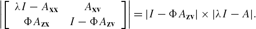
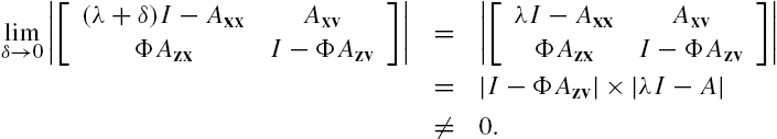
On the other hand, from Eq. (7.2) we have that ![]() . Substituting this relation into the last equation, we have that
. Substituting this relation into the last equation, we have that ![]() . Then, by Lemma 7.1 we can declare that system Σ is stable if and only if
. Then, by Lemma 7.1 we can declare that system Σ is stable if and only if
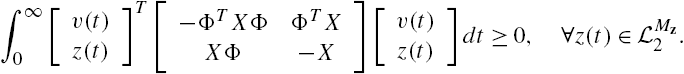
As in Theorem 7.2 we can prove that the above inequality is satisfied if ![]() for every
for every ![]() , which is equivalent to
, which is equivalent to
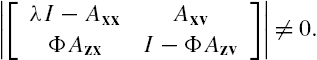
In addition, from the well-posedness assumption on each subsystem ![]() we can declare that the matrix
we can declare that the matrix
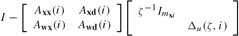
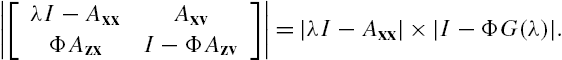
is of full normal rank. By Theorem 2.3 and the definition of the transfer function matrix ![]() straightforward algebraic manipulations show that Eq. (7.A.5) is equivalent to that for all
straightforward algebraic manipulations show that Eq. (7.A.5) is equivalent to that for all ![]() ,
, ![]() , and
, and ![]() ,
,
By Eq. (7.26) this inequality can be rewritten as
Substitute Eqs. (7.25) into this inequality. Note that to guarantee the satisfaction of Eq. (7.A.7) for each ![]() , it is necessary that this inequality is satisfied for
, it is necessary that this inequality is satisfied for ![]() . This means that
. This means that
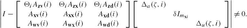
Combining these two equations, we can claim from Theorem 2.3 that Eq. (7.A.7) is equivalent to

Note that

Direct matrix operations show that the above inequality is further equivalent to
The proof can now be completed through a direct application of Definition 2.4 of the structured singular value. □
7.A.2 Proof of Theorem 7.4
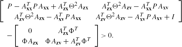
To prove Theorem 7.4, we first construct the following matrix inequality:
where X is a positive definite matrix with a compatible dimension. Assume that it is feasible.
Note that

Substitute this relation into Eq. (7.A.9). Straightforward matrix manipulations show that it is equivalent to

that is,
which can be reexpressed as

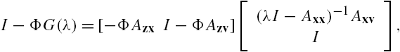
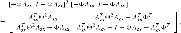
On the other hand, from Eqs. (7.42) and (7.47) direct but tedious matrix manipulations show that
Multiply both sides of Eq. (7.A.12) from left and right respectively by

Based on Eq. (7.A.13), we obtain the inequality
where
Note that the matrix 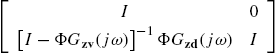 is of full rank at each
 ![]() . It is obvious that
. It is obvious that ![]() is also a positive number.
is also a positive number.
According to the Schur complement theorem (Lemma 2.4), the satisfaction of inequality (7.A.14) is equivalent to the satisfaction of the following two inequalities:
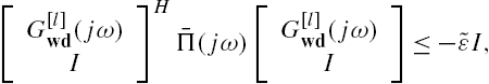

where δ is a very small positive number.
From the well-posedness assumption about the networked system we can declare that the matrix ![]() is of full rank at every complex value of the Laplace transform variable s. This implies that when inequality (7.A.15) is satisfied, there always exists a positive definite matrix X such that inequality (7.A.16) is also satisfied. As a matter of fact, we can even declaim that under such that a situation, there always exists a positive scalar x such that the positive definite matrix
is of full rank at every complex value of the Laplace transform variable s. This implies that when inequality (7.A.15) is satisfied, there always exists a positive definite matrix X such that inequality (7.A.16) is also satisfied. As a matter of fact, we can even declaim that under such that a situation, there always exists a positive scalar x such that the positive definite matrix ![]() satisfies inequality (7.A.16). To clarify this point, define the scalars
satisfies inequality (7.A.16). To clarify this point, define the scalars
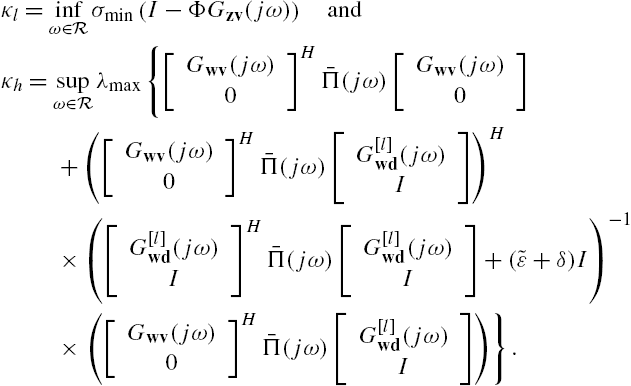
Then, from the well-posedness of the networked system and the satisfaction of inequality (7.A.15) we can directly claim that
Define the matrix
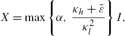
where α is an arbitrary positive number. Then, X is positive definite and satisfies inequality (7.A.16).
Therefore, feasibility of inequality (7.43) is equivalent to inequality (7.A.9) and to inequality (7.49). This completes the proof. □