
Attack Identification and Prevention in Networked Systems
Abstract
An essential requirement for a large-scale networked system to work properly is its safety. In this chapter, we investigate some preliminary issues in prevention and estimation of malicious and organized inputs to a networked system, which include detectability and identifiability of attacks, appropriate sensor distributions, and so on. We establish connections with system observability and with system transmission zeros. It has been made clear that accurate system model is quite important in both risk managements and attack building. We also discuss some recent quantitative methods developed for analyzing risks of a networked system.
Keywords
controllability; least squares estimates; observability; SCADA; security; state estimation; transmission zero
11.1 Introduction
A large-scale networked system usually consists of a great amount of subsystems, and these subsystems are often spatially distributed and far from each other geometrically. This asks for timely data exchanges among subsystems, which can be supported by advanced communication technologies, including both wired and wireless channels. Examples include electric power systems, unmanned vehicle systems, water supply networks, and so on.
Although integrations of several subsystems are greatly expected to increase performances of the whole system, they also provide more opportunities of being affected by malicious operators. There are many real world examples illustrating these possibilities, and in some cases, significant damages have been caused to the physical processes targeted by the attackers [1]. One example is the advanced computer worm Stuxnet, which happened in 2010 and infected some industrial control systems, reportedly leading to damages of approximately 1,000 centrifuges at these plants, although the attack itself was rather naive from a control engineer's point of view [2]. Another example is the Maroochy water breach in 2000 [3]. In this incident, an attacker managed to hack into some controllers that activate and deactivate some valves, which caused flooding of the grounds of a hotel, a park, and a river, with about a million liters of sewage. In 2003, the SQL Slammer worm attacked the Davis–Besse nuclear plant [4]. The recent multiple power blackouts in Brazil are also believed to be caused by malicious attacks [5].
Differently from faults and disturbances in a control system, which happen naturally and occasionally, attacks may happen in a well-organized way, simultaneously or sequentially over several spatial places of a large-scale networked system, with the objective to significantly violate performances of the system, or even to destroy the system itself. In other words, although faults also affect system behaviors, simultaneous events are usually not considered to be colluding. On the contrary, simultaneous attacks are often cooperative. In addition, faults are usually constrained by some physical dynamics and do not have an intent or objective, but attacks are usually not straightforwardly restricted by the dynamics of the plant physical process and/or chemical process, usually have a malicious objective, and often perform in a secrete way.
System safety is in fact not a new topic [6,7]. Particularly, in a power system, a supervisory control and data acquisition system, which is usually abbreviated as SCADA, is well developed and has been widely adopted. This system is originally designed to prevent electricity theft and to monitor abrupt voltage changes. In this system, measurement data of plant static outputs are used to estimate plant states, and the estimates are normally used in an internal control area of a transmission system operator. A basic assumption adopted in SCADA is that the system is in a steady-state behavior within its computation interval, which is usually of tens of seconds. When the plant states have a fast change during some alert or emergency situations, its estimation accuracy deteriorates drastically. Moreover, new power generation sources, such as large-scale wind power penetration, smart transmission devices, and so on have not been taken into account appropriately. In addition, inaccurate estimations about the state of a directly connected subsystem may cause some misleading estimates about system security and lead to a wrong decision of security control. These factors ask investigations on attack preventions using dynamic input–output data.
On the other hand, with the development of communication technologies and computer technologies, it is extensively anticipated that a plant and even subsystems of a plant are connected by some public communication networks, such as the world wide web and so on, to reduce hardware costs and increase maintenance flexibilities. In such a situation, a communication network becomes also an essential part of a networked system, such as that played by a physical plant and a digital feedback controller. When a system is connected by communication channels, many other possibilities arise for the system to be attacked. For example, it becomes easier for a hacker to insert some destructive disturbances in a more secrete way into a signal being transmitted in a communication channel [7–9]. In particular, a cyber-physical system usually suffers from some specific vulnerabilities, which do not exist in classical control systems and for which appropriate detection and identification techniques are required. For instance, the reliance on communication networks and standard communication protocols to transmit measurements and control packets increases the possibility of intentional and worst-case attacks against physical plants and/or the controller. On the other hand, information security methods, such as authentication, access control, message integrity, and so on, may not be adequate for a satisfactory protection of these attacks. Indeed, these security methods are only some passive ways to prevent a signal being disturbed during its transmissions. They do not exploit compatibilities of the received signals with the underlying physical/chemical process of the plant and/or the control mechanism. These characteristics may make them ineffective against an insider attack targeting the physical dynamics and/or the controller.
Generally, the dynamics of a networked system with possible attacks can be described as
where ![]() ,
, ![]() ,
, ![]() , and
, and ![]() respectively represent the plant state vector, output vector, input vector, and the vector consisting of possible attacks. Moreover,
respectively represent the plant state vector, output vector, input vector, and the vector consisting of possible attacks. Moreover, ![]() and
and ![]() are in general nonlinear functions that may be time varying. For a physical plant to work properly, there are usually some strict restrictions on its states. For example, in a water supply network, the levels of its reservoirs are in general restricted in some suitable ranges. The set consisting of these permissible plant states is called the plant safe region, whereas the complimentary set of the plant states is called the unsafe region. A plant is said to be safe if its state vector belongs to its safe region; otherwise, the plant is said to be unsafe. The objectives of the malicious attackers are often manipulating the plant state vector from its safe region to its unsafe region through adding an attack disturbance vector process
are in general nonlinear functions that may be time varying. For a physical plant to work properly, there are usually some strict restrictions on its states. For example, in a water supply network, the levels of its reservoirs are in general restricted in some suitable ranges. The set consisting of these permissible plant states is called the plant safe region, whereas the complimentary set of the plant states is called the unsafe region. A plant is said to be safe if its state vector belongs to its safe region; otherwise, the plant is said to be unsafe. The objectives of the malicious attackers are often manipulating the plant state vector from its safe region to its unsafe region through adding an attack disturbance vector process ![]() into the system with the smallest efforts, as well as to avoid being detected. In other words, to manipulate the plant from being safe to being unsafe in a theft and economic way. The input signal
into the system with the smallest efforts, as well as to avoid being detected. In other words, to manipulate the plant from being safe to being unsafe in a theft and economic way. The input signal ![]() is delivered from a controller through a communication network designed to make the plant work satisfactory. Due to the imperfectness of communication channels, this delivery may have some time delays and even failures and be corrupted by environment noises. Without detectors, the plant is usually impossible to distinguish the input vector
is delivered from a controller through a communication network designed to make the plant work satisfactory. Due to the imperfectness of communication channels, this delivery may have some time delays and even failures and be corrupted by environment noises. Without detectors, the plant is usually impossible to distinguish the input vector ![]() from that carrying the attack vector
from that carrying the attack vector ![]() . In other words, the attack vector
. In other words, the attack vector ![]() is usually injected into the input vector
is usually injected into the input vector ![]() possibly in a transmission process, and this injection combines these two vectors into a single vector that is input to the plant. Differently from external disturbances widely studied in control system analysis and synthesis, the attack vector
possibly in a transmission process, and this injection combines these two vectors into a single vector that is input to the plant. Differently from external disturbances widely studied in control system analysis and synthesis, the attack vector ![]() is usually not random. More precisely, it might be designed with a clear objective using some measurements of the plant output vector
is usually not random. More precisely, it might be designed with a clear objective using some measurements of the plant output vector ![]() .
.
When ![]() , the networked system described by Eqs. (11.1) and (11.2) is said to be in its normal situation, and the associated trajectories of its state and output vectors are said to be in their nominal behavior. Otherwise, the system is said to be in an abnormal situation, and the corresponding trajectories of its state and output vectors are said to be in their abnormal behavior. The objective of attack estimation is to clarify whether or not the system is in its normal situation using measurements of its output vector, whereas the objective of attack identification is to estimate the amount and positions of attackers when the system is in an abnormal situation. Generally, these two problems are dealt with through investigating characteristics of the residues of some detectors.
, the networked system described by Eqs. (11.1) and (11.2) is said to be in its normal situation, and the associated trajectories of its state and output vectors are said to be in their nominal behavior. Otherwise, the system is said to be in an abnormal situation, and the corresponding trajectories of its state and output vectors are said to be in their abnormal behavior. The objective of attack estimation is to clarify whether or not the system is in its normal situation using measurements of its output vector, whereas the objective of attack identification is to estimate the amount and positions of attackers when the system is in an abnormal situation. Generally, these two problems are dealt with through investigating characteristics of the residues of some detectors.
Taking into account that for nonlinear dynamic systems, there still does not exist a general analysis and/or synthesis method, our attention is restricted to linear systems in this chapter, in which both the function ![]() of Eq. (11.1) and the function
of Eq. (11.1) and the function ![]() of Eq. (11.2) are linear. This significantly reduces mathematical difficulties in handling the attack estimation and prevention problems, keeping the associated results significant and relevant from an engineering viewpoint. With this simplification, the input vector
of Eq. (11.2) are linear. This significantly reduces mathematical difficulties in handling the attack estimation and prevention problems, keeping the associated results significant and relevant from an engineering viewpoint. With this simplification, the input vector ![]() can be removed from the model, as its existence does not affect conclusions on either attack identification or attack prevention due to the linearities of the system.
can be removed from the model, as its existence does not affect conclusions on either attack identification or attack prevention due to the linearities of the system.
In this chapter, we first discuss attack identification and prevention using static data, which has been extensively adopted in large-scale electric power networks. Afterward, relations between system observability and attack prevention are investigated. With these relations, estimation and identification of attacks are respectively dealt with, as well as the relations between system security and optimal sensor placements. Further research topics will also be briefly discussed.
To clarify basic concepts and ideas, rather than the general model of a networked system given by Eqs. (3.25) and (3.26), which has been discussed in several chapters of this book, in this chapter the state-space model of Eq. (3.1) is utilized.
11.2 The SCADA System
Very possibly, the most successful attack estimator until now is the SCADA system, which is originally designed to protect an electricity network from working in an unsafe region. In this system, the plant is assumed to be in steady state, and its state vector is estimated from its output measurements using a least squares method. Clearly, to let this system work properly, it is necessary that the number of sensors in the plant is not smaller than the dimension of its state vector. Otherwise, the output of the associated attack detector cannot be uniquely determined, which will invalidate its usefulness. Generally, the more the sensors the plant has, the better the detection performance the system has.
When the plant is linear and works in its steady state, and only output measurements are utilized in estimating its state vector, the relations between the plant outputs and states, described by Eq. (11.2), can be expressed in a much simpler way given as follows:
In this equation, a vector ![]() is introduced to represent measurement noises. For simplicity, we assume that its mathematical expectation is constantly equal to zero, whereas its covariance matrix is constantly equal to the identity matrix. As pointed out before, to get a physically meaningful estimate about the plant states, it is necessary that the dimension of the output vector
is introduced to represent measurement noises. For simplicity, we assume that its mathematical expectation is constantly equal to zero, whereas its covariance matrix is constantly equal to the identity matrix. As pointed out before, to get a physically meaningful estimate about the plant states, it is necessary that the dimension of the output vector ![]() is not smaller than that of the state vector
is not smaller than that of the state vector ![]() . This means that the output matrix
. This means that the output matrix ![]() has more rows than columns.
has more rows than columns.
When no attacks are available, a reasonable estimate about the plant state vector, denoted ![]() , which is extensively adopted and widely called a least squares estimate, is
, which is extensively adopted and widely called a least squares estimate, is
With this estimate, the predicted plant output ![]() and its prediction errors
and its prediction errors ![]() are respectively
are respectively
Obviously, to make this estimate physically meaningful, it is necessary that the matrix ![]() is of full column rank, which guarantees the existence of the inverse of
is of full column rank, which guarantees the existence of the inverse of ![]() . This condition can be satisfied through an appropriate sensor placement in the plant.
. This condition can be satisfied through an appropriate sensor placement in the plant.
When the measurement error vector ![]() has a normal distribution, we can easily prove that
has a normal distribution, we can easily prove that ![]() has a
has a ![]() distribution. Hence, an anomaly detector, which is based on a quantity of the residue of plant output measurement, can be defined as
distribution. Hence, an anomaly detector, which is based on a quantity of the residue of plant output measurement, can be defined as
which is in fact the SCADA system [6]. Obviously, this detector shares the same form of the output prediction error in the normal situation that is given by ![]() . In this system,
. In this system, ![]() is utilized to decide whether or not there exists an attack in the networked system. When its value is greater than a prescribed threshold, it is believed that an attack exists. Otherwise, there are no attacks in the networked system [6,7].
is utilized to decide whether or not there exists an attack in the networked system. When its value is greater than a prescribed threshold, it is believed that an attack exists. Otherwise, there are no attacks in the networked system [6,7].
This anomaly detector is usually efficient in detecting a single attack which caused a significant change in one of the plant output measurements. However, when a coordinated malicious attack exists in the plant and may cause simultaneous change of several plant output measurements, very possibly, this detector does not work quite well. For example, assume that there is a coordinated attack ![]() satisfying
satisfying
This is possible if the attackers appropriately select their attack places and strategies and coordinate their actions. Under such a situation, we have that the output of the anomaly detector satisfies the following equalities:
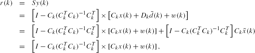
that is, no matter how large the magnitude of an element in the vector ![]() is, the output of the anomaly detector, that is,
is, the output of the anomaly detector, that is, ![]() , does not change. This invalidates its capabilities of detecting the attacks satisfying Eq. (11.8).
, does not change. This invalidates its capabilities of detecting the attacks satisfying Eq. (11.8).
Note that when the plant is linear and the input signal ![]() is constantly set to zero, by Eq. (11.1) its state evolutions can be expressed as
is constantly set to zero, by Eq. (11.1) its state evolutions can be expressed as
In the plant steady state, we have that ![]() . Hence,
. Hence,
which may be very far from the steady state of the plant without an attack, which is equal to zero by the adopted assumption that ![]() . In fact, when the attack of Eq. (11.8) is applied,
. In fact, when the attack of Eq. (11.8) is applied,
where ![]() stands for the pseudo-inverse of the matrix
stands for the pseudo-inverse of the matrix ![]() .1 As each element of the vector
.1 As each element of the vector ![]() can be arbitrarily large in magnitude without being detected by the anomaly detector, this equation implies that an appropriate selection of either the matrix
can be arbitrarily large in magnitude without being detected by the anomaly detector, this equation implies that an appropriate selection of either the matrix ![]() or the matrix
or the matrix ![]() , or both of them, may cause a significant change of the plant states, which are capable of deriving the plant to its unsafe region. On the other hand, through choices of attack positions in a networked system, a selection of either the matrix
, or both of them, may cause a significant change of the plant states, which are capable of deriving the plant to its unsafe region. On the other hand, through choices of attack positions in a networked system, a selection of either the matrix ![]() or the matrix
or the matrix ![]() can be realized in a relatively easy way, provided that the attackers have accurate information on the system model, which is mostly about the system output matrix
can be realized in a relatively easy way, provided that the attackers have accurate information on the system model, which is mostly about the system output matrix ![]() in this case.
in this case.
These conclusions are valid even if the plant is not in its steady state. In addition, numerical studies show that the attack in the form (11.8), which is extensively called stealthy attack, is usually sparse [6,7].
To analyze the security of a networked system, some security indices have also been introduced. When the plant is also time invariant, the following index ![]() is suggested in [7] to measure the security degree of the plant jth output measurement:
is suggested in [7] to measure the security degree of the plant jth output measurement:
where to make the expressions more concise, the temporal variable k has been omitted from the system matrices. Moreover, ![]() stands for the jth row vector of the output matrix C.
stands for the jth row vector of the output matrix C.
From its definition it is clear that when an attacker is intended to change the plant jth output measurement without being detected by the SCADA system, ![]() is in fact the minimum number of plant output measurements that he/she needs compromise. The smaller this index, the easier the jth plant output measurement to be attacked by a stealthy attack, that is, an attack that cannot be detected in principle. This means that knowledge about this security index for all the plant output measurements may provide some useful information about the security vulnerabilities of the networked system, which may be helpful in protecting the networked system with restricted resources.
is in fact the minimum number of plant output measurements that he/she needs compromise. The smaller this index, the easier the jth plant output measurement to be attacked by a stealthy attack, that is, an attack that cannot be detected in principle. This means that knowledge about this security index for all the plant output measurements may provide some useful information about the security vulnerabilities of the networked system, which may be helpful in protecting the networked system with restricted resources.
Although the security index is significant from an engineering viewpoint, the associated optimization problem itself cannot be easily solved. In fact, this minimization problem has been proven to be NP-hard, and various modifications have been suggested as an alternative. One example is to replace the vector 0-norm with the vector 1-norm.
11.3 Attack Prevention and System Transmission Zeros
The previous section illustrates briefly the SCADA system, which uses only plant output measurements to detect whether or not there are attacks in the plant. The attack detection method is quite simple, but it reveals almost all essential issues in attack preventions: an attacker usually intends to significantly violate or even destroy a system in a secrete way, whereas a detector should be efficient in revealing all the attacks as soon as possible. This implies that there may exist close relations between attack preventions and system observability. In this section, we clarify these relations under the situation in which both the detector and the attacker have accurate knowledge about the plant dynamics.
As general conclusions are still not available for nonlinear time-varying systems, our attention is also restricted to linear and time-invariant systems in this section. We assume that an attacker is intended to alter the states of a plant through injecting some exogenous inputs on the basis of the system matrices of the plant at each time. In addition, the attacker is assumed to have unrestricted computation capabilities. An attacker with these characteristics is called an omniscient attacker. Under these assumptions, stealthy colluding attacks are closely related to plant transmission zeros.
Assume that the dynamics of a networked system with possible attacks is described as
As in the previous section, here ![]() represents an attack disturbance. Once again, we assume that
represents an attack disturbance. Once again, we assume that ![]() ,
, ![]() , and
, and ![]() . Noting that the plant is assumed to be linear, it is not necessary to include control signals in the adopted model.
. Noting that the plant is assumed to be linear, it is not necessary to include control signals in the adopted model.
To simplify discussions, we assume throughout the rest of this chapter that the above state space model is a minimal realization, that is, it is both controllable and observable. Note that if the system is not controllable, then a decomposition can divide its state space into the direct sum of controllable and uncontrollable subspaces, and the system state vector can be manipulated by an attacker only when it is in the controllable subspace. On the other hand, if the system is unobservable, then the system state space can be decomposed into the direct sum of observable and unobservable subspaces. As the part of a state vector belonging to the unobservable subspace does not have any influence on the plant output vector, variations of this part cannot be detected by the plant output vectors. That is, under such a situation, there always exist attacks that cannot be detected and therefore cannot be identified by monitoring only these plant outputs. This observation means that the aforementioned minimal realization assumption is reasonable.
Another assumption adopted in the rest of this chapter is that the matrix ![]() is of full column rank, which is constituted from the system input matrix B and its direct feedthrough matrix D. This is necessary for the identifiability of attacks, noting that if this matrix is not of full column rank, then different attacks may cause the same value of the vector
is of full column rank, which is constituted from the system input matrix B and its direct feedthrough matrix D. This is necessary for the identifiability of attacks, noting that if this matrix is not of full column rank, then different attacks may cause the same value of the vector ![]() . More precisely, for an arbitrary
. More precisely, for an arbitrary ![]() , it is obvious from the definition of the null space of a matrix that
, it is obvious from the definition of the null space of a matrix that

In addition, when the matrix ![]() is not of full column rank,
is not of full column rank, ![]() has at least one nonzero vector as its element. Under such a situation, it is clear from Eqs. (11.14) and (11.15) that these different attacks lead to the same trajectory of the system state vector and to the same trajectory of the system output vector. Obviously, this is not an appreciative property in attack detection and/or attack identification.
has at least one nonzero vector as its element. Under such a situation, it is clear from Eqs. (11.14) and (11.15) that these different attacks lead to the same trajectory of the system state vector and to the same trajectory of the system output vector. Obviously, this is not an appreciative property in attack detection and/or attack identification.
Similarly to those in the SCADA system, an attack detector, which is sometimes also called an attack monitor, exploits only plant dynamics and output measurements to reveal the existence of attacks and identify their positions. Hence, an attack cannot be detected in principle if the associated plant output measurements are consistent with those without any attacks. On the contrary, if an attack causes a plant output measurement that has some characteristics different from those in regular/normal situations, some methods may be developed to detect this attack. Note that the output of a plant depends on both its initial conditions and external inputs. To clarify this dependence, rather than ![]() ,
, ![]() is used more often in the following discussions. Here,
is used more often in the following discussions. Here, ![]() belongs to the set
belongs to the set ![]() and represents the value of the plant state vector at the time instant
and represents the value of the plant state vector at the time instant ![]() .
.
Similarly, ![]() is sometimes adopted to indicate the dependence of the state vector on its initial values and on the input vector sequence
is sometimes adopted to indicate the dependence of the state vector on its initial values and on the input vector sequence ![]() .
.
Definition 11.1
From an engineering point of view, this definition means that a detector cannot be constructed if the plant outputs associated with some attacks are completely the same as those due to modifications of plant initial conditions. One of the basic motivations behind this definition is that plant initial conditions are usually not exactly known in many applications, which makes the mapping from a plant input series to a plant output series not bijective and therefore leaves opportunities for an attacker to inject destructive disturbances.
In addition, to detect whether or not there exists an attack in a networked system, it is usually necessary for a detector to determine where the attack is from if it exists. This leads to an attack identification problem and requires to construct a detector that has capabilities of identifying attack locations. As attacks in a networked system are usually sparse, only a few elements of the attack vector ![]() are usually not constantly equal to zero. Hence, some upper bounds can be put on the number of colluding attackers. Here, we assume that at most K attackers collude in one attack.
are usually not constantly equal to zero. Hence, some upper bounds can be put on the number of colluding attackers. Here, we assume that at most K attackers collude in one attack.
Definition 11.2
(Unidentifiable attack) Concerning the system described by Eqs. (11.14) and (11.15), an attack vector sequence ![]() with K elements not constantly zero is unidentifiable if for each initial state vector
with K elements not constantly zero is unidentifiable if for each initial state vector ![]() , there exist at least one other initial state vector
, there exist at least one other initial state vector ![]() and one other attack vector sequence
and one other attack vector sequence ![]() with
with ![]() elements not constantly zero, where
elements not constantly zero, where ![]() , such that at every time instant
, such that at every time instant ![]() , the plant output satisfies
, the plant output satisfies ![]() .
.
Similarly to an undetectable attack, an unidentifiable attack cannot be identified because another attack can generate completely the same plant output, which makes plant outputs alone not sufficiently informative in distinguishing these attacks.
Let ![]() denote a set consisting of K nonzero positive integers that belong to the set
denote a set consisting of K nonzero positive integers that belong to the set ![]() , where q stands for the dimension of the attack vector
, where q stands for the dimension of the attack vector ![]() . Associating with this set, define the attack set
. Associating with this set, define the attack set ![]() in which an entry of the attack vector
in which an entry of the attack vector ![]() is not constantly set to zero only if it is in the row whose number is one of the elements of the set
is not constantly set to zero only if it is in the row whose number is one of the elements of the set ![]() . More precisely, assume that
. More precisely, assume that ![]() with
with ![]() for each
for each ![]() . Then,
. Then,
where ![]() stands for the ith row element of the attack vector
stands for the ith row element of the attack vector ![]() .
.
An attack set is undetectable if there exists at least one undetectable attack in that set. Similarly, an attack set is unidentifiable if there exists at least one unidentifiable attack in that set. As the attack set ![]() only provides information about the position, in which an attack is injected into the networked system, which is completely the same as that of the set
only provides information about the position, in which an attack is injected into the networked system, which is completely the same as that of the set ![]() , sometimes the set
, sometimes the set ![]() is also called as an attack set. In other words, when an attack from the attack set
is also called as an attack set. In other words, when an attack from the attack set ![]() is injected into the networked system described by Eqs. (11.14) and (11.15),
is injected into the networked system described by Eqs. (11.14) and (11.15), ![]() and
and ![]() in these equations can be respectively rewritten as
in these equations can be respectively rewritten as ![]() and
and ![]() , where
, where ![]() is constituted from the columns of the matrix B whose numbers are consistent with the elements of the set
is constituted from the columns of the matrix B whose numbers are consistent with the elements of the set ![]() , whereas
, whereas ![]() is constituted from the columns of the matrix D whose numbers are consistent with the elements of the set
is constituted from the columns of the matrix D whose numbers are consistent with the elements of the set ![]() . In addition,
. In addition, ![]() is a K-dimensional real-valued vector.
is a K-dimensional real-valued vector.
In [9], a different attack detection problem is formulated and investigated. It is assumed there that only sensors or actuators of a networked system are attacked, and a characterization is given for the maximum number of attacks that can be detected and corrected, which is expressed as a function of the plant state transition matrix and the plant output matrix. Although this problem formulation appears to be different from that given in Definition 11.1, they are actually closely related to each other [7].
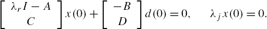
From linearity assumption of the networked system and Definition 11.1 it is obvious that an attack ![]() is undetectable if and only if there exists a plant initial state vector
is undetectable if and only if there exists a plant initial state vector ![]() such that
such that
The latter is closely related to some fundamental properties of a dynamic system. In fact, Eq. (11.16) has completely the same form as that of the conditions adopted in the definition of the zero dynamics of a system. More precisely, under some weak conditions, the equality in this equation can be satisfied if and only if the attack ![]() only stimulates the zero dynamics of the networked system [10,11]. Due to these relations, we can establish an algebraic criterion to verify whether or not an attack set is undetectable.
only stimulates the zero dynamics of the networked system [10,11]. Due to these relations, we can establish an algebraic criterion to verify whether or not an attack set is undetectable.
Similarly, we can straightforwardly prove that an attack ![]() with K elements that are not constantly zero is unidentifiable if and only if there exist a plant initial state vector
with K elements that are not constantly zero is unidentifiable if and only if there exist a plant initial state vector ![]() and an attack
and an attack ![]() with
with ![]() elements in
elements in ![]() that is not constantly zero and the integer
that is not constantly zero and the integer ![]() satisfying
satisfying ![]() such that
such that
Note that Eqs. (11.16) and (11.17) are quite similar in their forms. It is not hard to understand that attack identification is once again closely related to transmission zeros of a networked system, which leads to an easily verifiable algebraic condition for an unidentifiable attack set.
11.3.1 Zero Dynamics and Transmission Zeros
These discussions reveal that both attack detection and attack identification are in fact a verification problem on the existence of an initial state vector and an input sequence that make the plant output vector be constantly equal to zero, which is closely related to zero dynamics and therefore to transmission zeros of a system. To illustrate these relations, the following conclusions are first established for a discrete-time system, which are similar to the results about continuous-time systems given in [10,11].
Lemma 11.1
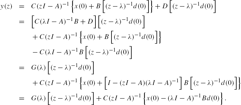
Let ![]() be the transfer function matrix with minimal realization given by Eqs. (11.14) and (11.15). If the system input vector process
be the transfer function matrix with minimal realization given by Eqs. (11.14) and (11.15). If the system input vector process ![]() is of the form
is of the form ![]() for each
for each ![]() and the system initial conditions satisfy
and the system initial conditions satisfy ![]() , in which λ is a constant scalar not equal to any eigenvalue of the matrix A, and
, in which λ is a constant scalar not equal to any eigenvalue of the matrix A, and ![]() is a constant vector with compatible dimension. Then for an arbitrary integer
is a constant vector with compatible dimension. Then for an arbitrary integer ![]() , the system output vector process
, the system output vector process ![]() can be expressed as
can be expressed as
Proof
When λ is not an eigenvalue of the matrix A, the matrix ![]() is invertible, which means that the condition
is invertible, which means that the condition ![]() is well defined. Note that when a system has a minimal realization of Eqs. (11.14) and (11.15), the
is well defined. Note that when a system has a minimal realization of Eqs. (11.14) and (11.15), the ![]() -transformation of its output vector process
-transformation of its output vector process ![]() can be expressed as
can be expressed as
Hence, when ![]() for each
for each ![]() , we have that
, we have that
Therefore, the condition ![]() leads to the following equality:
leads to the following equality:
Recall that λ is a constant scalar. The proof can now be completed through taking the inverse ![]() -transform of the vector-valued function
-transform of the vector-valued function ![]() . □
. □
From Lemma 11.1 it is clear that if ![]() belongs to the null space of
belongs to the null space of ![]() , then when the system initial state vector is set as
, then when the system initial state vector is set as ![]() , the plant output vector
, the plant output vector ![]() is constantly equal to zero for each
is constantly equal to zero for each ![]() . However, it is worth mentioning that when λ is a real scalar and
. However, it is worth mentioning that when λ is a real scalar and ![]() is a real-valued vector, both
is a real-valued vector, both ![]() with any
with any ![]() and
and ![]() are real-valued vectors, which can be realized in principle in actual engineering problems, noting that both the state transition matrix A and the system input matrix B are real valued. However, when either λ is a complex scalar or
are real-valued vectors, which can be realized in principle in actual engineering problems, noting that both the state transition matrix A and the system input matrix B are real valued. However, when either λ is a complex scalar or ![]() is a complex-valued vector, the associated
is a complex-valued vector, the associated ![]() with
with ![]() and/or
and/or ![]() may also be complex valued. This may make the associated values not be realizable by any actual system input vector process and/or any system initial states.
may also be complex valued. This may make the associated values not be realizable by any actual system input vector process and/or any system initial states.
When λ is equal to an eigenvalue of the state transition matrix A, the discussions become more complicated. However, with the results of Theorem 2.5, similar results can still be obtained. On the other hand, using a concept called system matrix, similar results can also be established without distinguishing whether or not λ is an eigenvalue of the state transition matrix A, which are given in the following Lemma 11.2.
To guarantee the existence of a nontrivial input vector process ![]() and a nontrivial initial state vector
and a nontrivial initial state vector ![]() such that all the conditions of Lemma 11.1 are satisfied and the plant output vector process is constantly equal to zero, it is necessary that the matrix
such that all the conditions of Lemma 11.1 are satisfied and the plant output vector process is constantly equal to zero, it is necessary that the matrix ![]() is not of full column rank. When the system is of single input and single output, it is obvious that λ must be one of the zeros of its transfer function, as the minimal realization assumption does not permit the existence of a zero in the transfer function that is equal to one of its poles. The situation becomes much more complicated when the system is of multiple inputs and multiple outputs. In this case, even if its state space model is a minimal realization, there still exists possibility that some of its zeros and some of its poles share the same value. To clarify the mathematical descriptions of a system zero and its relations to the zero dynamics of the system, the following concepts are required.
is not of full column rank. When the system is of single input and single output, it is obvious that λ must be one of the zeros of its transfer function, as the minimal realization assumption does not permit the existence of a zero in the transfer function that is equal to one of its poles. The situation becomes much more complicated when the system is of multiple inputs and multiple outputs. In this case, even if its state space model is a minimal realization, there still exists possibility that some of its zeros and some of its poles share the same value. To clarify the mathematical descriptions of a system zero and its relations to the zero dynamics of the system, the following concepts are required.
Definition 11.3
A vector ![]() is called weakly unobservable if there exists an input vector sequence
is called weakly unobservable if there exists an input vector sequence ![]() , such that the corresponding output vector sequence
, such that the corresponding output vector sequence ![]() is constantly equal to zero, that is,
is constantly equal to zero, that is, ![]() for each
for each ![]() .
.
Denote by ![]() the set consisting of all weakly unobservable vectors of a system. From the linearity of the system we can straightforwardly proven that this set is actually a subspace of
the set consisting of all weakly unobservable vectors of a system. From the linearity of the system we can straightforwardly proven that this set is actually a subspace of ![]() . Due to this reason, the set
. Due to this reason, the set ![]() is sometimes called the weakly unobservable subspace of the system [11,12]. In fact, if we define a subspace
is sometimes called the weakly unobservable subspace of the system [11,12]. In fact, if we define a subspace ![]() with
with ![]() , as
, as

then it is obvious from the definition of this subspace sequence that
In addition, we can directly prove that there exists a nonnegative integer ![]() such that
such that
Let ![]() and
and ![]() satisfy
satisfy
The existence of these matrices is shown in [11]. Then we can prove that, for each ![]() , an input vector sequence
, an input vector sequence ![]() that satisfies
that satisfies
can be parameterized so that, for an arbitrary ![]() ,
,
where ![]() is an arbitrary real vector sequence with compatible dimension. Moreover, we can also prove that if
is an arbitrary real vector sequence with compatible dimension. Moreover, we can also prove that if ![]() and
and ![]() with
with ![]() is an associated input vector sequence such that
is an associated input vector sequence such that ![]() for each
for each ![]() , then the associated state vector sequence
, then the associated state vector sequence ![]() , denoted
, denoted ![]() , satisfies
, satisfies ![]() for each
for each ![]() .
.
Some other properties of this weakly unobservable subspace can be found, for example, in [11,12].
The concept of zero dynamics of a system is established on the basis of its weakly unobservable subspace.
Definition 11.4
The zero dynamics of a system is also connected to its weakly unobservable subspace through its system matrix, a concept suggested originally by Rosenbrock [11,13].
Lemma 11.2
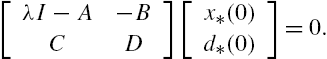
Concerning the system described by Eqs. (11.14) and (11.15), assume that the matrix ![]() is of full column rank. Define its system matrix
is of full column rank. Define its system matrix
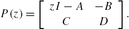
Suppose that there exist a vector ![]() and a vector
and a vector ![]() such that at least one of these two vectors is not equal to zero, and at a real value of the complex variable z, denoted λ, the following equality is satisfied:
such that at least one of these two vectors is not equal to zero, and at a real value of the complex variable z, denoted λ, the following equality is satisfied:
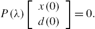
Then for each ![]() , the input vector sequence
, the input vector sequence ![]() satisfies both
satisfies both ![]() and
and ![]() .
.
Proof
Note that the system defined by Eqs. (11.14) and (11.15) is well defined. This means that for a fixed initial state vector ![]() and each input vector sequence
and each input vector sequence ![]() , there are only one state vector sequence
, there are only one state vector sequence ![]() and only one output vector sequence
and only one output vector sequence ![]() that satisfy these two equations simultaneously.
that satisfy these two equations simultaneously.
When condition (11.23) is satisfied, define ![]() as
as ![]() for every
for every ![]() . Then, we can straightforwardly prove that
. Then, we can straightforwardly prove that
Assume now that, for an integer i with ![]() , Eq. (11.14) is satisfied by
, Eq. (11.14) is satisfied by ![]() and
and ![]() . Then, we can straightforwardly prove that
. Then, we can straightforwardly prove that

that is, when ![]() , the aforementioned state vector process and input vector process also satisfy Eq. (11.14). Therefore,
, the aforementioned state vector process and input vector process also satisfy Eq. (11.14). Therefore, ![]() and
and ![]() satisfy this equation for every
satisfy this equation for every ![]() . Hence,
. Hence, ![]() is the solution to this difference equation with its initial state vector
is the solution to this difference equation with its initial state vector ![]() and input vector process
and input vector process ![]() .
.
On the other hand, note that, for each ![]() ,
,
provided that the vectors ![]() and
and ![]() satisfy conditions (11.23). Therefore,
satisfy conditions (11.23). Therefore, ![]() , and for each
, and for each ![]() ,
,
Now, assume that λ takes a complex value. Denote its real and imaginary parts respectively by ![]() and
and ![]() . Recall that the matrices A, B, C, and D and the vectors
. Recall that the matrices A, B, C, and D and the vectors ![]() and
and ![]() are real valued. Satisfaction of Eq. (11.23) implies that
are real valued. Satisfaction of Eq. (11.23) implies that
In addition, note that

which means that

If ![]() , then it is necessary that
, then it is necessary that ![]() . As the matrix
. As the matrix ![]() is assumed to be of full column rank,
is assumed to be of full column rank, ![]() and the first subequation in the above equation imply that the vector
and the first subequation in the above equation imply that the vector ![]() is also equal to zero. This is a contradiction with the requirement that at least one of the vectors
is also equal to zero. This is a contradiction with the requirement that at least one of the vectors ![]() and
and ![]() is not equal to zero. Hence,
is not equal to zero. Hence, ![]() , that is, λ takes a real value.
, that is, λ takes a real value.
These arguments show that if there is λ satisfying Eq. (11.23), then it is necessary that this λ is real valued. Hence, ![]() is real valued for each
is real valued for each ![]() . This completes the proof. □
. This completes the proof. □
Clearly, a real vector satisfying Eq. (11.23) belongs to the weakly unobservable subspace ![]() of the system.
of the system.
From the proof of Lemma 11.2 it is obvious that if both the system initial state vector ![]() and its input vector sequence
and its input vector sequence ![]() are allowed to take complex values, then the associated results are valid even when the complex variable z takes a complex value that satisfies Eq. (11.23). In this case, both
are allowed to take complex values, then the associated results are valid even when the complex variable z takes a complex value that satisfies Eq. (11.23). In this case, both ![]() and
and ![]() may be complex vectors, which will lead to a complex-valued sequence
may be complex vectors, which will lead to a complex-valued sequence ![]() that makes the associated system output vector sequence constantly equal to zero.
that makes the associated system output vector sequence constantly equal to zero.
On the other hand, Lemma 11.2 does not require that λ is different from every eigenvalue of the state transition matrix A, which makes its results more general than those on system zero dynamics derived from Lemma 11.1. In fact, if λ is not an eigenvalue of the state transition matrix A, then Eq. (11.23) straightforwardly leads to ![]() , which can be rewritten as
, which can be rewritten as ![]() . This is completely in the same form as the condition obtained from Lemma 11.1 for the system output vector sequence constantly equal to zero. These observations imply that when λ is not an eigenvalue of the matrix A, the conditions of Lemma 11.2 are equal to those derived from Lemma 11.1. Hence, we can regard that Lemma 11.2 includes some conclusions of Lemma 11.1 as its particular case.
. This is completely in the same form as the condition obtained from Lemma 11.1 for the system output vector sequence constantly equal to zero. These observations imply that when λ is not an eigenvalue of the matrix A, the conditions of Lemma 11.2 are equal to those derived from Lemma 11.1. Hence, we can regard that Lemma 11.2 includes some conclusions of Lemma 11.1 as its particular case.
To guarantee the existence of a nonzero vector ![]() and/or a nonzero vector
and/or a nonzero vector ![]() such that Eq. (11.23) is satisfied, it is necessary that the matrix
such that Eq. (11.23) is satisfied, it is necessary that the matrix ![]() is not of full column rank. A complex value λ at which the system matrix
is not of full column rank. A complex value λ at which the system matrix ![]() defined by Eq. (11.22) is not of full column rank is called a transmission zero of this system, which is an extension of a zero in a transfer function of a single-input single-output system to a zero of the transfer function matrix of a multiple-input multiple-output system [10,13].
defined by Eq. (11.22) is not of full column rank is called a transmission zero of this system, which is an extension of a zero in a transfer function of a single-input single-output system to a zero of the transfer function matrix of a multiple-input multiple-output system [10,13].
Various methods have been developed for the computation of the transmission zeros of a multiple-input multiple-output system, among which one of most widely adopted methods appears to be the approach based on the so-called McMillan–Smith form [10,11]. In addition, the proof of the lemma reveals that to construct an actually realizable system initial state vector and an actually realizable system input vector process such that the system output vector process is constantly equal to zero, real-valued transmission zeros must be considered.
Our discussions show that if a system has a real transmission zero, then there certainly exist a real-valued initial state vector and a real-valued input vector sequence that lead to a constantly zero output vector sequence. However, it is still not clear that if there is a real-valued initial state vector ![]() and a real-valued input vector sequence
and a real-valued input vector sequence ![]() such that the associated output vector sequence
such that the associated output vector sequence ![]() is constantly zero, whether or not the system must have at least one real transmission zero.
is constantly zero, whether or not the system must have at least one real transmission zero.
To attack this problem, we need the following concept.
Definition 11.5
When a system is linear, it is obvious from the definition that a necessary and sufficient condition for its left invertibility is that ![]() if and only if
if and only if ![]() . For the linear time-invariant system described by Eqs. (11.14) and (11.15) that has a minimal realization, let
. For the linear time-invariant system described by Eqs. (11.14) and (11.15) that has a minimal realization, let ![]() denote its transfer function matrix
denote its transfer function matrix ![]() . It has been proven that the following statements are equivalent to each other [11]:
. It has been proven that the following statements are equivalent to each other [11]:
- • This system is left invertible.
- • There exists a rational matrix-valued function
 such that
  , that is, the transfer function matrix
  has a left inverse.
 - • The system matrix
 defined in Eq. (11.22) has a rank of
  for all but finitely many
  .
. - • Let
 denote the weakly unobservable subspace of the system. Then

Related to the concept of weak observability, there is also a concept called strong observability.
Definition 11.6
For a linear time invariant system, the following results have been established in [11].
Lemma 11.3

From Definitions 11.3 and 11.6 it is obvious that a system is strongly observable if and only if its weakly unobservable subspace is constituted only from the zero vector. It has also been proven that, for the linear time-invariant system of Eqs. (11.14) and (11.15), its strong observability is equivalent to that, for each real matrix F with compatible dimension, the matrix pair ![]() is always observable [11].
is always observable [11].
Based on these results, the following conclusions are derived, which reveal situations under which the weakly unobservable subspace of a system is not restricted only to the zero vector.
Theorem 11.1
Proof
Assume that the system has a real transmission zero. Then by Lemma 11.2 there certainly exists a nonzero initial state vector satisfying the requirements.
Now, assume that all the transmission zeros of the system are complex. Let λ be any one of them. Then there exist vectors ![]() and
and ![]() such that at least one of them is not equal to zero and the following equality is satisfied:
such that at least one of them is not equal to zero and the following equality is satisfied:
Recall that all the system parameter matrices A, B, C, and D are real. Taking the conjugates of both sides of this equation, we obtain the following equality:

As ![]() does not equal zero, it is obvious that the vector
does not equal zero, it is obvious that the vector ![]() is not a zero vector either. These imply that
is not a zero vector either. These imply that ![]() is also a transmission zero of the system.
is also a transmission zero of the system.
Define ![]() as
as ![]() ,
, ![]() . Let
. Let ![]() and
and ![]() denote respectively the
denote respectively the ![]() -transformations of the sequences
-transformations of the sequences ![]() and
and ![]() . Moreover, let
. Moreover, let ![]() and
and ![]() denote respectively the
denote respectively the ![]() -transformations of the output vector sequences
-transformations of the output vector sequences ![]() and
and ![]() . According to the proof of Lemma 11.2, we have that
. According to the proof of Lemma 11.2, we have that
Define ![]() and
and ![]() further as
further as
Then, both ![]() and
and ![]() with
with ![]() are real valued and therefore can be realized in principle.
are real valued and therefore can be realized in principle.
Let ![]() denote the
denote the ![]() -transformation of the output vector sequence associated with the system initial state vector
-transformation of the output vector sequence associated with the system initial state vector ![]() and the input vector sequence
and the input vector sequence ![]() . Then by Eq. (11.19) we have that
. Then by Eq. (11.19) we have that

We can therefore declare from Eq. (11.26) that, for each ![]() ,
,
On the contrary, assume that the system described by Eqs. (11.14) and (11.15) does not have a transmission zero but there is a nonzero initial state vector ![]() such that there exists an input sequence
such that there exists an input sequence ![]() that makes
that makes ![]() for every
for every ![]() . Then, for arbitrary
. Then, for arbitrary ![]() , the matrix
, the matrix

is of full column rank. Hence

By Lemma 11.3 this system is strongly observable. Hence, if there is an input sequence ![]() that makes
that makes ![]() for every
for every ![]() , then
, then ![]() . This contradicts the assumption
. This contradicts the assumption ![]() . Therefore, the system must have some transmission zeros.
. Therefore, the system must have some transmission zeros.
This completes the proof. □
Different from Lemma 11.2, the transmission zero in the theorem is not required to be real. On the other hand, both the initial state vector and the input vector sequence are required to be real.
11.3.2 Attack Prevention
From the results in the previous subsection it is clear that a linear time-invariant system is left invertible if and only if its transfer function matrix is of full normal column rank. This observation leads further to the following conclusions.
Proof
Assume that a transfer function matrix ![]() is not of FNCR. Then there exists a nonzero vector α such that, for each
is not of FNCR. Then there exists a nonzero vector α such that, for each ![]() , the following equality is satisfied:
, the following equality is satisfied:
Let ![]() be a real matrix quadruplex that satisfies
be a real matrix quadruplex that satisfies ![]() and associates with a state space model having a minimal realization. Take an arbitrary real scalar λ that is not an eigenvalue of the matrix A and denote the associated real and imaginary parts of the vector α by
and associates with a state space model having a minimal realization. Take an arbitrary real scalar λ that is not an eigenvalue of the matrix A and denote the associated real and imaginary parts of the vector α by ![]() and
and ![]() , respectively. Then, the Eq. (11.29) means that the following two equalities are satisfied:
, respectively. Then, the Eq. (11.29) means that the following two equalities are satisfied:
Note that ![]() is equivalent to
is equivalent to ![]() , that is, the assumption
, that is, the assumption ![]() implies that at least one of
implies that at least one of ![]() and
and ![]() is not equal to zero.
is not equal to zero.
Assume that ![]() . Then, the first equality of Eq. (11.30) can be equivalently rewritten as
. Then, the first equality of Eq. (11.30) can be equivalently rewritten as
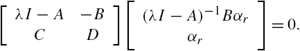
Note that both vectors ![]() and
and ![]() are real. Moreover, the vector
are real. Moreover, the vector 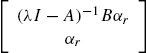 is not a zero vector. By Lemma 11.2 there always exist a nonzero
 ![]() and an input vector sequence
and an input vector sequence ![]() , not constantly equal to zero, such that the output vector process of the LTI system, which can be expressed as
, not constantly equal to zero, such that the output vector process of the LTI system, which can be expressed as ![]() , is constantly equal to zero for each
, is constantly equal to zero for each ![]() . Hence the system is not attack detectable/identifiable.
. Hence the system is not attack detectable/identifiable.
When ![]() , the same arguments show that the system is not attack detectable/identifiable.
, the same arguments show that the system is not attack detectable/identifiable.
This completes proof. □
These observations reveal that the problem of attack preventions is not trivial only when the associated system is left invertible.
With these preparations on system zero dynamics, we discuss now conditions respectively for the detectability and identifiability of attacks in a networked system.
Theorem 11.2

Proof
Assume that the matrix ![]() is not of full column rank at a particular real value of the complex variable λ, denoted
is not of full column rank at a particular real value of the complex variable λ, denoted ![]() . Then, there exist vectors
. Then, there exist vectors ![]() and
and ![]() such that at least one of these two vectors is not a zero vector and
such that at least one of these two vectors is not a zero vector and
As all the involved matrices, that is, the state transition matrix A, the input matrix ![]() , the output matrix C, and the direct feedthrough matrix
, the output matrix C, and the direct feedthrough matrix ![]() , and the scalar
, and the scalar ![]() are real valued, we can assume, without any loss of generality, that both vectors
are real valued, we can assume, without any loss of generality, that both vectors ![]() and
and ![]() are real valued. In fact, if they are not real valued, then denote their real and imaginary parts respectively by
are real valued. In fact, if they are not real valued, then denote their real and imaginary parts respectively by ![]() ,
, ![]() ,
, ![]() , and
, and ![]() . Then Eqs. (11.33) and (11.34) imply that
. Then Eqs. (11.33) and (11.34) imply that
Note that by their definitions all the vectors ![]() ,
, ![]() ,
, ![]() , and
, and ![]() are real valued. Moreover, at least one of them is not equal to zero. Reasonability of the adopted assumption immediately follows.
are real valued. Moreover, at least one of them is not equal to zero. Reasonability of the adopted assumption immediately follows.
We now can declare the undetectability of the attack set ![]() through a direct application of Lemma 11.2.
through a direct application of Lemma 11.2.
Assume now that the system matrix ![]() is not of full column rank at a particular complex value
is not of full column rank at a particular complex value ![]() . If the system is not left invertible, then according to the aforementioned arguments, we can declare that the system is not detectable of the attack set
. If the system is not left invertible, then according to the aforementioned arguments, we can declare that the system is not detectable of the attack set ![]() .
.
Now, assume that the system is left invertible. Then from Theorem 11.1 we can declare that the attack set ![]() is not detectable.
is not detectable.
Assume that the attack set ![]() is detectable. Then, by Corollary 11.1 its transfer function matrix must be of full normal column rank. From this observation and the definition of attack detectability, this system cannot have any transmission zero.
is detectable. Then, by Corollary 11.1 its transfer function matrix must be of full normal column rank. From this observation and the definition of attack detectability, this system cannot have any transmission zero.
This completes proof. □
From Eqs. (11.33) and (11.34) we can also see that for the existence of an undetectable attack, it is necessary that the cardinality of the attack set is sufficiently large [7]. On the other hand, it is possible to improve attack detectability of a networked system through introducing state feedback into the system. The motivations are that a state feedback can modify transmission zeros of a system and the feedback gain can be designed with objectives that are unknown to an attacker.
Similarly, we have the following criterion for attack identifiability of the networked system described by Eqs. (11.14) and (11.15).
Theorem 11.3
Proof
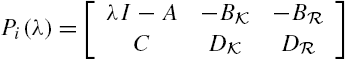
Assume that at a particular real value of the complex variable λ, denoted ![]() , the matrix-valued function
, the matrix-valued function ![]() is not of full column rank. Then there exist vectors
is not of full column rank. Then there exist vectors ![]() ,
, ![]() , and
, and ![]() such that at least one of these three vectors is not a zero vector, and
such that at least one of these three vectors is not a zero vector, and
Using the same arguments as in the proof of Theorem 11.2, we can assume, without loss of any generality, that the vectors ![]() ,
, ![]() , and
, and ![]() are real valued. Then by Lemma 11.2 there exist an initial state vector
are real valued. Then by Lemma 11.2 there exist an initial state vector ![]() and an input vector sequence
and an input vector sequence ![]() ,
, ![]() , such that the output vector sequence
, such that the output vector sequence ![]() of the following system is constantly equal to zero.
of the following system is constantly equal to zero.
Moreover, at least either the initial state vector ![]() is not a zero vector, or the input vector sequence
is not a zero vector, or the input vector sequence ![]() is not constantly equal to zero. Note that both matrices
is not constantly equal to zero. Note that both matrices ![]() and
and ![]() are of full column rank. Direct algebraic manipulations show that, for this plant initial state vector
are of full column rank. Direct algebraic manipulations show that, for this plant initial state vector ![]() , there exist an attack
, there exist an attack ![]() with K elements in
with K elements in ![]() not constantly zero, an attack
not constantly zero, an attack ![]() with
with ![]() elements in
elements in ![]() not constantly zero, and the integer
not constantly zero, and the integer ![]() satisfying
satisfying ![]() such that
such that
that is, the attack set ![]() is not identifiable.
is not identifiable.
By the same token as that adopted in the proof of Theorem 11.2, we can prove that even if the aforementioned ![]() takes a particular complex value, the system is also unidentifiable with respect to the attack set
takes a particular complex value, the system is also unidentifiable with respect to the attack set ![]() .
.
This completes the proof. □
On the basis of geometric linear system theories, some graph theoretic conditions have also been established for the existence of an undetectable attack set in a networked system and for the existence of an unidentifiable attack set in a networked system. These conditions depend only on system structures and are valid for almost all system parameters when the networked system has a compatible structure. A system property with these characteristics is extensively called generic and has the advantage of strong robustness against parametric modeling errors [14]. When the initial state vector of a networked system is known, it is proven that if the attack-state-output graph is sufficiently connected, then undetectable attacks do not exist in almost all structurally compatible networked systems. When the initial state vector is not known for a networked system, the criterion becomes more complicated, and left invertibility of the system may be required. Detailed discussions can be found, for example, in [7,8].
11.4 Detection of Attacks
In the above section, we developed some criteria to verify whether or not an attack can be detected or identified. These criteria are closely related to the transmission zeros of a networked system and can be verified in principle. When the scale of the system is large, however, computations of its transmission zeros may be computationally prohibitive and/or numerically unstable. This means that further efforts are required to develop a computationally attractive method for verifying attack detectability and identifiability. To achieve this objective, the methods given in Chapter 3 may be helpful, in which structure information is explicitly and efficiently utilized in the verification of controllability and observability of a large-scale networked system, noting that both the system matrix ![]() of Eq. (11.32) and the system matrix
of Eq. (11.32) and the system matrix ![]() of Eq. (11.37) have a similar form of the matrix-valued polynomial
of Eq. (11.37) have a similar form of the matrix-valued polynomial ![]() of Eq. (3.29). In this section, we investigate how to detect an attack using a centralized observer.
of Eq. (3.29). In this section, we investigate how to detect an attack using a centralized observer.
The design of an attack detector consists of a discrete-time modified Luenberger observer, which is sometimes also called a residual filter, with its input being the plant output measurements ![]() and its output being a residual signal
and its output being a residual signal ![]() :
:
where the matrix L is usually called the gain of the observer, which is selected to make the matrix ![]() stable, that is, all its eigenvalues have a magnitude smaller than 1. When the matrix pair
stable, that is, all its eigenvalues have a magnitude smaller than 1. When the matrix pair ![]() is observable, the existence of a desirable gain matrix L is always guaranteed. The residue signal
is observable, the existence of a desirable gain matrix L is always guaranteed. The residue signal ![]() is used to detect the existence of an attack. Ideally, this signal is constantly equal to zero if and only if there do not exist any attacks in the networked system. As the initial state vector of the observer also affects the residual signal, these expectations cannot be satisfied in general, and some modifications are required to develop a practically meaningful criterion to check the existence of an attack. However, we have the following theoretical results on the aforementioned residual filter.
is used to detect the existence of an attack. Ideally, this signal is constantly equal to zero if and only if there do not exist any attacks in the networked system. As the initial state vector of the observer also affects the residual signal, these expectations cannot be satisfied in general, and some modifications are required to develop a practically meaningful criterion to check the existence of an attack. However, we have the following theoretical results on the aforementioned residual filter.
Theorem 11.4
Concerning the system described by Eqs. (11.14) and (11.15), assume that an attack set ![]() is detectable and the initial state vector of the system, that is,
is detectable and the initial state vector of the system, that is, ![]() , is known. Assume also that the initial state vector of the residual filter described by Eqs. (11.42) and (11.43), that is,
, is known. Assume also that the initial state vector of the residual filter described by Eqs. (11.42) and (11.43), that is, ![]() , is set to
, is set to ![]() , and the gain matrix L is selected such that the matrix
, and the gain matrix L is selected such that the matrix ![]() is stable. Then, the residual signal of the filter is constantly equal to zero if and only if the attack disturbance is constant equal to zero.
is stable. Then, the residual signal of the filter is constantly equal to zero if and only if the attack disturbance is constant equal to zero.
Proof
Define the vector-valued function ![]() . Then from Eqs. (11.14), (11.15), (11.42), and (11.43) we can straightforwardly prove that
. Then from Eqs. (11.14), (11.15), (11.42), and (11.43) we can straightforwardly prove that

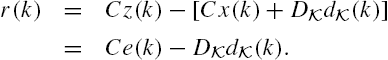
When the initial state vector of the detector is set to be the same value of the initial state vector of the system, that is, ![]() , we have that
, we have that ![]() . Hence, when the matrix
. Hence, when the matrix ![]() has all its eigenvalues being smaller than 1 in magnitude and the attack disturbances do not exist, that is,
has all its eigenvalues being smaller than 1 in magnitude and the attack disturbances do not exist, that is, ![]() , it is obvious from Eq. (11.44) that the error vector sequence
, it is obvious from Eq. (11.44) that the error vector sequence ![]() with
with ![]() is also constantly equal to zero. This further implies that the output vector of the detector, that is, the residual vector
is also constantly equal to zero. This further implies that the output vector of the detector, that is, the residual vector ![]() is also constantly equal to zero when the temporal variable k takes any value from the set
is also constantly equal to zero when the temporal variable k takes any value from the set ![]() .
.
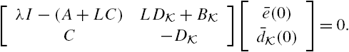
Now assume that there exists a nonzero attack vector sequence ![]() such that the output of the attack detector described by Eqs. (11.42) and (11.43) is constantly equal to zero. Then by Theorem 11.4 there must exist at least one
such that the output of the attack detector described by Eqs. (11.42) and (11.43) is constantly equal to zero. Then by Theorem 11.4 there must exist at least one ![]() , one vector
, one vector ![]() , and one vector
, and one vector ![]() such that at least one of these two vectors is not equal to zero and
such that at least one of these two vectors is not equal to zero and
Note that

Note also that the matrix ![]() is invertible for every real-valued matrix L with compatible dimension. It is obvious that the satisfaction of Eq. (11.46) is equivalent to the satisfaction of the equation
is invertible for every real-valued matrix L with compatible dimension. It is obvious that the satisfaction of Eq. (11.46) is equivalent to the satisfaction of the equation

which contradicts the assumption that the attack set ![]() is detectable. This completes the proof. □
is detectable. This completes the proof. □
Although the results of Theorem 11.4 are promising, the system initial state vector ![]() is usually not known exactly. Under such a situation, the condition
is usually not known exactly. Under such a situation, the condition ![]() can generally not be satisfied properly for the initial state vector of the residual filter, and
can generally not be satisfied properly for the initial state vector of the residual filter, and ![]() may be selected with some arbitrariness. This means that even if there do not exist attacks in the networked system, the residual signal
may be selected with some arbitrariness. This means that even if there do not exist attacks in the networked system, the residual signal ![]() may not be constantly equal to zero. However, it can be proven that when the networked system has not been attacked, the residual signal
may not be constantly equal to zero. However, it can be proven that when the networked system has not been attacked, the residual signal ![]() asymptotically converges to zero with the increment of the temporal variable k. On the other hand, measurement errors and external random disturbances are usually unavoidable in actual networked systems, which means that even if the conditions of Theorem 11.4 are perfectly satisfied, the residual signal
asymptotically converges to zero with the increment of the temporal variable k. On the other hand, measurement errors and external random disturbances are usually unavoidable in actual networked systems, which means that even if the conditions of Theorem 11.4 are perfectly satisfied, the residual signal ![]() may not be constantly equal to zero and some statistical hypothesis verification methodologies appear necessary for the determination of whether or not there are attacks in the networked system. In addition to these, parametric uncertainties and unmodeled dynamics usually exist in the model of Eqs. (11.14) and (11.15). Hence, in actual implementations of attack detections, in addition to construct a stable residual filter, the gain matrix L should be selected to reduce sensitivities of the residual signal
may not be constantly equal to zero and some statistical hypothesis verification methodologies appear necessary for the determination of whether or not there are attacks in the networked system. In addition to these, parametric uncertainties and unmodeled dynamics usually exist in the model of Eqs. (11.14) and (11.15). Hence, in actual implementations of attack detections, in addition to construct a stable residual filter, the gain matrix L should be selected to reduce sensitivities of the residual signal ![]() to modeling errors while keeping it satisfactorily sensitive to attacks. Furthermore, for a large-scale networked system, it is usually more attractive to implement an attack detector in a distributed way using only local subsystem output measurements. Detailed discussions on these issues are given in various literature, for example, [9], [8], and [7].
to modeling errors while keeping it satisfactorily sensitive to attacks. Furthermore, for a large-scale networked system, it is usually more attractive to implement an attack detector in a distributed way using only local subsystem output measurements. Detailed discussions on these issues are given in various literature, for example, [9], [8], and [7].
11.5 Identification of Attacks
In actual applications, it is usually not only necessary to know whether or not there exists an attack in a networked system, but also essential to know where the attack is from when it exists. Differently from attack detection, attack identification is computationally much more difficult due to its combinatorial characteristics, although their essential treatments are the same. In fact, it has been proven in [8] that attack identifications are generally NP hard with respect to the number of colluding attackers. More precisely, the identification of an attack from the attack set ![]() usually requires a combinatorial procedure, noting that even when the number q of attackers is known, the actual attack is only one of the
usually requires a combinatorial procedure, noting that even when the number q of attackers is known, the actual attack is only one of the ![]() possible attacks. To identify this attack, each possibility must be considered, and for each possible attack, a residual filter needs be designed. When the attack set is identifiable, there exists one and only one residual filter whose outputs are constantly equal to zero. It is this residual filter that indicates the actual attack.
possible attacks. To identify this attack, each possibility must be considered, and for each possible attack, a residual filter needs be designed. When the attack set is identifiable, there exists one and only one residual filter whose outputs are constantly equal to zero. It is this residual filter that indicates the actual attack.
Unlike the residual filter in attack detection, the model of Eqs. (11.14) and (11.15) is not straightforwardly utilized in constructing the residual filters in attack identification. Usually, the design of these residual filters consists of three steps. First, a transformation is applied to the plant output vector to construct a vector without any attacks. Second, a state transformation is performed to divide the plant state vector into two parts, one affected by attack disturbances and the other is free from attack disturbances. The third step is to construct a residual filter with the transformed plant output vector and the transformed plant state vector that are not affected by attack disturbances, which is completely the same as that in the construction procedure for attack detections.
Now, we discuss the first step, in which the attack identification problem for the networked system described by Eqs. (11.14) and (11.15) is converted to that of a modified system in which the associated system output vector is not attacked.
For this purpose, let ![]() denote the pseudo-inverse of the matrix
denote the pseudo-inverse of the matrix ![]() . Define an auxiliary networked system as
. Define an auxiliary networked system as
Then, we have the following conclusions.
Lemma 11.4
Proof
According to Theorem 11.3, if the attack set ![]() is identifiable for the networked system described by Eqs. (11.14) and (11.15), then for each attack set
is identifiable for the networked system described by Eqs. (11.14) and (11.15), then for each attack set ![]() with its cardinality not greater than that of the attack set
with its cardinality not greater than that of the attack set ![]() , the following system matrix
, the following system matrix ![]() is of full column rank at each complex number λ:
is of full column rank at each complex number λ:
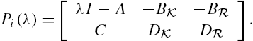
It is equivalent to that the matrix ![]() defined as
defined as
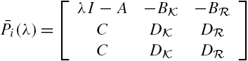
is of full column rank at each complex number λ.
Multiplying both sides of the above equation from the left by ![]() , we have that
, we have that

Note that

Moreover, the matrix

is always invertible, and it is obvious that the above equations mean that the matrix-valued function
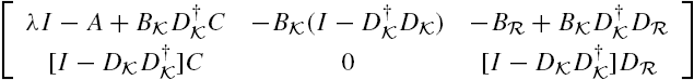
is also of full column rank at each complex λ. It can therefore be concluded from Theorem 11.3 that the attack set ![]() is also identifiable for the networked system described by Eqs. (11.48) and (11.49).
is also identifiable for the networked system described by Eqs. (11.48) and (11.49).
On the contrary, if the attack set ![]() is identifiable for the networked system described by Eqs. (11.48) and (11.49), then similar arguments show that this attack set is also identifiable for the networked system described by Eqs. (11.14) and (11.15).
is identifiable for the networked system described by Eqs. (11.48) and (11.49), then similar arguments show that this attack set is also identifiable for the networked system described by Eqs. (11.14) and (11.15).
This completes the proof. □
To construct a residual signal that is able to identify an attack, the state space model of Eqs. (11.48) and (11.49) is further transformed. To develop this transformation, however, some concepts and results are needed from geometric control theory, which can be found, for example, in [11,12].
Definition 11.7
Assume that the dynamics of a discrete-time and linear time-invariant system can be described by the following state space model:

where ![]() ,
, ![]() , and
, and ![]() denote respectively the state vector, input vector, and output vector of the system. Moreover, assume that
denote respectively the state vector, input vector, and output vector of the system. Moreover, assume that ![]() is a subspace of
is a subspace of ![]() . If
. If
then this subspace is said to be ![]() -conditioned invariant.
-conditioned invariant.
A conditioned invariant subspace is closely related to estimator designs. A well-known result is that the smallest ![]() -conditioned invariant subspace that contains the subspace
-conditioned invariant subspace that contains the subspace ![]() as its subset is the largest subspace in the state space
as its subset is the largest subspace in the state space ![]() of the system, which can be estimated in the presence of an unknown input sequence
of the system, which can be estimated in the presence of an unknown input sequence ![]() . This conclusion is obviously of great significance in engineering, as it clarifies situations for the existence of a state estimator with unknown inputs. Another well-known result is that the null space of the observability matrix, that is,
. This conclusion is obviously of great significance in engineering, as it clarifies situations for the existence of a state estimator with unknown inputs. Another well-known result is that the null space of the observability matrix, that is,

which gives all the initial state vectors that result in a zero system output when there do not exist any external inputs are an ![]() -conditioned invariant subspace.
-conditioned invariant subspace.
It has been proven that for each ![]() -conditioned invariant subspace
-conditioned invariant subspace ![]() , there exists at least one real matrix L such that
, there exists at least one real matrix L such that
that is, an output injection matrix that renders this subspace invariant.
To apply these concepts and results to the system described by Eqs. (11.48) and (11.49), let ![]() denote the smallest
denote the smallest ![]() -conditioned invariant subspace that contains
-conditioned invariant subspace that contains ![]() as its subspace. Moreover, let L be a matrix that satisfies
as its subspace. Moreover, let L be a matrix that satisfies
Existence of a desirable matrix L is guaranteed by the properties of the subspace ![]() . Furthermore, let T be a nonsingular square matrix satisfying
. Furthermore, let T be a nonsingular square matrix satisfying

where ![]() is a matrix of full row rank. We can prove using geometric control theories that a desirable matrix T always exists [8,11,12]. As a matter of fact, the matrix T can be constituted from a basis of the subspace
is a matrix of full row rank. We can prove using geometric control theories that a desirable matrix T always exists [8,11,12]. As a matter of fact, the matrix T can be constituted from a basis of the subspace ![]() and a basis of the quotient subspace
and a basis of the quotient subspace ![]() [11,12].
[11,12].
With the aforementioned matrix transformation, we can establish the following conclusions.
Lemma 11.5


Proof
Assume that the networked system described by Eqs. (11.56) and (11.57) is attack identifiable for the attack set ![]() . Then, for each complex number λ and each attack set
. Then, for each complex number λ and each attack set ![]() with its attacker number not greater than k, if
with its attacker number not greater than k, if
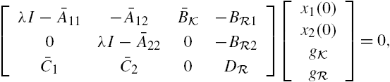
then it is necessary that all the vectors ![]() ,
, ![]() ,
, ![]() , and
, and ![]() are zero vectors, that is,
are zero vectors, that is,
Note that

We therefore have that

As the matrix T is regular by its definition, it is obvious that both two matrices
are well defined and are of full rank. We can therefore claim from Eqs. (11.58) and (11.61) that the matrix

is also of full column rank for each complex number λ and each attack set ![]() with its attacker number not greater than that of the attack set
with its attacker number not greater than that of the attack set ![]() . Hence, from Lemma 11.4 and Theorem 11.3 we can declare attack identifiability for the attack set
. Hence, from Lemma 11.4 and Theorem 11.3 we can declare attack identifiability for the attack set ![]() in the networked system described by Eqs. (11.14) and (11.15).
in the networked system described by Eqs. (11.14) and (11.15).
Similar arguments show that if the attack set ![]() is identifiable for the networked system described by Eqs. (11.14) and (11.15), then it is also identifiable for the networked system described by Eqs. (11.56) and (11.57).
is identifiable for the networked system described by Eqs. (11.14) and (11.15), then it is also identifiable for the networked system described by Eqs. (11.56) and (11.57).
This completes the proof. □
Note that in the state space model of Eqs. (11.56) and (11.57), the state vector ![]() is completely isolated from any attack disturbances. Using this property, a residual filter can be constructed as
is completely isolated from any attack disturbances. Using this property, a residual filter can be constructed as
This residual filter is very similar to that for attack detections given in the previous section, except that the output vector ![]() is replaced by a modified output vector
is replaced by a modified output vector ![]() . Obviously, this modification is removing
. Obviously, this modification is removing ![]() from the output vector
from the output vector ![]() with the purpose of constructing an output vector that is not affected by any attack disturbances, noting that the substate vector
with the purpose of constructing an output vector that is not affected by any attack disturbances, noting that the substate vector ![]() is independent of the attack disturbance vector
is independent of the attack disturbance vector ![]() and
and
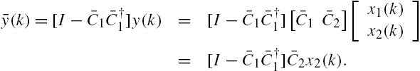
With this residual filter, we have the following results.
Theorem 11.5
Let the networked system be described by Eqs. (11.14) and (11.15). Assume that the attack set ![]() is identifiable. Moreover, assume that the initial state vector
is identifiable. Moreover, assume that the initial state vector ![]() of the networked system is known. Furthermore, assume that the initial state vector of the residual filter described by Eqs. (11.62)–(11.64) is set as
of the networked system is known. Furthermore, assume that the initial state vector of the residual filter described by Eqs. (11.62)–(11.64) is set as ![]() and that the gain matrix
and that the gain matrix ![]() is selected such that the matrix
is selected such that the matrix ![]() is stable. Then the residual signal
is stable. Then the residual signal ![]() of the above filter is constantly equal to zero if and only if both matrices
of the above filter is constantly equal to zero if and only if both matrices ![]() and
and ![]() coincide with those of the actual colluding attackers.
coincide with those of the actual colluding attackers.
Proof
Using the state vector ![]() of the attack identifier described by Eqs. (11.62)–(11.64), define the new state vector
of the attack identifier described by Eqs. (11.62)–(11.64), define the new state vector ![]() evolving as
evolving as
Moreover, define the error vector ![]() , in which two suberror vectors
, in which two suberror vectors ![]() and
and ![]() are respectively defined as
are respectively defined as ![]() and
and ![]() . Then on the basis of Eqs. (11.14), (11.15), (11.62)–(11.64), and (11.65), straightforward algebraic manipulations show that
. Then on the basis of Eqs. (11.14), (11.15), (11.62)–(11.64), and (11.65), straightforward algebraic manipulations show that

When ![]() is set to be equal to
is set to be equal to ![]() , the definition of the suberror vector
, the definition of the suberror vector ![]() implies that
implies that ![]() . As the residual signal
. As the residual signal ![]() is not directly affected by the attack disturbances
is not directly affected by the attack disturbances ![]() , and the matrix
, and the matrix ![]() is selected to assure that the magnitude of each eigenvalue of the matrix
is selected to assure that the magnitude of each eigenvalue of the matrix ![]() is smaller than 1, this residual signal
is smaller than 1, this residual signal ![]() is constantly equal to zero, provided that the attack set is
is constantly equal to zero, provided that the attack set is ![]() . This completes the proof. □
. This completes the proof. □
In case that there exist modeling errors in the adopted state space model, and/or there are random disturbances in the networked system, and/or the initial state vector ![]() is not exactly known, observations in attack detections are also valid for the above attack identification methods. On the other hand, from the above results it is clear that to identify an attack, it is necessary to construct at least one residual filter for each possible attack. This might be not feasible when the number K is large.
is not exactly known, observations in attack detections are also valid for the above attack identification methods. On the other hand, from the above results it is clear that to identify an attack, it is necessary to construct at least one residual filter for each possible attack. This might be not feasible when the number K is large.
Similarly to the attack detector discussed in the previous section, it is also possible to realize the above attack identifier in a distributed way. The details are not included in this book. Some preliminary results can be found in [8,9].
11.6 System Security and Sensor/Actuator Placement
The previous sections make it clear that to detect and/or identify an attack in networked systems, system observability is an essential property. In Chapter 3, we have discussed how to verify observability of a large-scale networked system and how many sensors are required to construct an observable networked system. However, it is usually not sufficient in actual engineering to only detect and/or identify an attack. A general requirement is to achieve this objective in an allowed time period after the occurrence of an attack, if not in the shortest time period. In fact, the longer the time is needed to detect/identify an attack, the larger the damages the attack may bring.
Note that both attack detection and attack identification depend on a residual generator. As system initial states cannot be known exactly in general and both modeling errors and external disturbances are usually unavoidable in actual applications, the time period and/or data length needed to detect/identify an attack depend heavily on the performances of that residual generator in its robustness against modeling errors and its capabilities of reducing influences from external disturbances. From the results of Section 11.5 it is clear that this residual generator can be easily rewritten into a form of the Luenberger observer discussed in Chapter 4, which includes the Kalman filter as its particular form. On the other hand, recall that the Kalman filter is optimal when the plant is linear and the external disturbances are normally distributed and when the sensitivity penalization-based robust state estimator given in Chapter 4 has completely the same form as that of the Kalman filter. It is interesting from both theoretical aspects and application aspects to investigate relations among estimation performances of the Kalman filter, the number of sensors, and the length of system output measurements [15]. A dual problem is about relations about control efforts, the number of actuators and optimal control performances, which is also an interesting topic in the analysis and synthesis of networked systems [16,17]. In fact, an attacker often intends to destroy a system with minimal efforts in a stealthy way, whereas a controller usually wants to improve system performances with the smallest energy consumptions.
In this section, we investigate a sensor placement problem and an actuator placement problem, both of them related closely to system security.
From a mathematical viewpoint, both sensor placement problems and actuator placement problems can be regarded as set function optimizations. When a sensor placement problem is under investigation, a set ![]() is usually adopted to denote the set consisting of all potential positions of a networked system in which a sensor can be placed, whereas the function
is usually adopted to denote the set consisting of all potential positions of a networked system in which a sensor can be placed, whereas the function ![]() represents metric measuring factors like the best performances that a state estimator can achieve with the measurements from several sensors belonging to a set
represents metric measuring factors like the best performances that a state estimator can achieve with the measurements from several sensors belonging to a set ![]() , the costs of these sensors, and so on. Then, when there are restrictions on the number of sensors in a networked system, say, it does not exceed k, a sensor placement problem may be mathematically described as
, the costs of these sensors, and so on. Then, when there are restrictions on the number of sensors in a networked system, say, it does not exceed k, a sensor placement problem may be mathematically described as
Here ![]() stands for the number of elements in the set
stands for the number of elements in the set ![]() . Basically, this is a finite combinatorial optimization problem, which can be solved in principle through exhausting all possible sensor sets that have its element number not greater than k and comparing their associated cost function values. When the number of subsystems in a networked system is large, as possibilities of sensor locations in general increase exponentially with the subsystem number, such a brute-force-based method is usually computationally prohibitive.
. Basically, this is a finite combinatorial optimization problem, which can be solved in principle through exhausting all possible sensor sets that have its element number not greater than k and comparing their associated cost function values. When the number of subsystems in a networked system is large, as possibilities of sensor locations in general increase exponentially with the subsystem number, such a brute-force-based method is usually computationally prohibitive.
Similar statements are valid for actuator placements.
To deal with these sensor/actuator placement problems, assume that the dynamics of a discrete time and linear time-variant system can be described by the following state space model:
Once again, here, ![]() ,
, ![]() , and
, and ![]() denote respectively the state vector, input vector, and output vector of the system. Moreover, assume that
denote respectively the state vector, input vector, and output vector of the system. Moreover, assume that ![]() is a subspace of
is a subspace of ![]() .
.
11.6.1 Some Properties of the Kalman Filter
It is now widely known that when a plant is linear and its external disturbances are normally distributed, the Kalman filter is the optimal state estimator under the criterion of mean squares errors [18,19]. Recent studies, however, show that when mean squares errors are adopted in the determination of optimal sensor locations, the associated optimization problem generally does not have the submodularity property and is in general NP-hard. Moreover, the widely adopted greedy heuristic algorithm may perform arbitrarily poorly, and there does not exist a constant-factor (polynomial-time) approximation algorithm [20,21].
To deal with the problem of appropriately locating sensors for a networked system, in this section, we investigate relations among estimation error, data length, and plant output number in the Kalman filtering. As only stochastic properties of ![]() affect estimation accuracies of the Kalman filter [18,19,22], we can assume without any loss of generality that
affect estimation accuracies of the Kalman filter [18,19,22], we can assume without any loss of generality that ![]() . To simplify mathematical expressions, this assumption is adopted throughout this and next subsections. Moreover, we assume that the system initial conditions, process disturbances, and measurement errors are white and uncorrelated. More precisely:
. To simplify mathematical expressions, this assumption is adopted throughout this and next subsections. Moreover, we assume that the system initial conditions, process disturbances, and measurement errors are white and uncorrelated. More precisely:
- •
 ,
,  , and
, and  are uncorrelated with each other for
  ;
; - • and are uncorrelated with
 and
and  for every nonnegative integer
  ;
; - •
 and
and  for each
  ;
; - •
 ,
,  , and
, and  with
with  for every nonnegative integer k.
Using the same arguments as in the derivation of Eq. (3.6), we can show straightforwardly from Eqs. (11.69) and (11.70) that, for arbitrary nonnegative integers k and ![]() with
with ![]() , the following equality is valid:
, the following equality is valid:

where
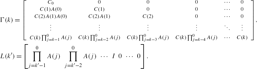
If ![]() ,
, ![]() , and
, and ![]() are normally distributed, then we can declare from Eq. (11.71) that
are normally distributed, then we can declare from Eq. (11.71) that
is also normally distributed, which is equivalent to that
are jointly normally distributed.
For simplicity, denote the vectors
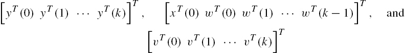
respectively by ![]() ,
, ![]() , and
, and ![]() . Then Eq. (11.71) can be rewritten as follows:
. Then Eq. (11.71) can be rewritten as follows:
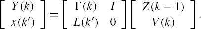
In addition, from the system output vector measurements ![]() ,
, ![]() , the best estimate of the system state vector
, the best estimate of the system state vector ![]() under the criterion of mean squares errors, denoted
under the criterion of mean squares errors, denoted ![]() , has been proven to have the following closed-form expression [18,19,22]:
, has been proven to have the following closed-form expression [18,19,22]:
that is,
under the constraints of Eq. (11.71).
Based on this relation and the adopted assumptions on the external disturbance process ![]() and the measurement error process
and the measurement error process ![]() , direct algebraic manipulations show that
, direct algebraic manipulations show that
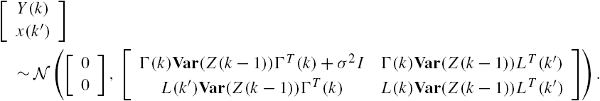
Concerning joint normal distributions, the following result is well known [23,24].
Lemma 11.6

On the basis of Eqs. (11.73) and (11.72) and Lemma 11.6, the following equality can be straightforwardly established:

Recall that when a linear space is constituted from n-dimensional random vectors with zero mean and finite covariance matrix, an inner product can be defined as
Obviously, the norm induced from this inner product is consistent with the cost function adopted in the optimization problem of Eq. (11.74), that is, the mean squares errors. Hence, from the projection-based optimization condition [25,26] we have that
Denote the estimation error vector ![]() by
by ![]() . From this equality and Eq. (11.75) direct algebraic operations show that
. From this equality and Eq. (11.75) direct algebraic operations show that
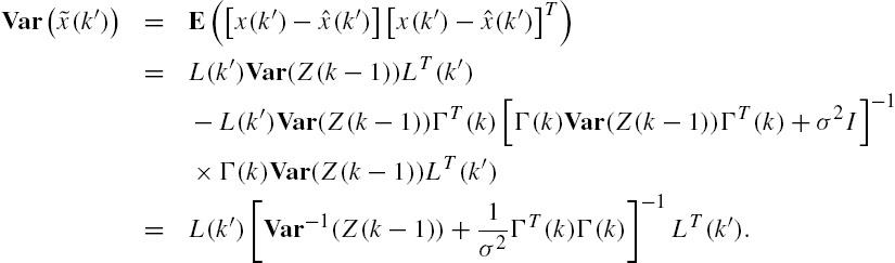
A recursive realization of Eqs. (11.76) and (11.78) is the well-known Kalman filter [18,19]. Rather than the recursive formula of the Kalman filter, which is given by Eqs. (4.8) and (4.9), expression (11.78) for the covariance matrix of estimation errors appears to be much more convenient in the analysis of the relations among sensor positions, sensor number, measurement data length, and estimation accuracy.
Define the random variable
Recall that the random vector ![]() is normally distributed. On the other hand, it is clear from Eqs. (11.72) and (11.76) that the random vector
is normally distributed. On the other hand, it is clear from Eqs. (11.72) and (11.76) that the random vector ![]() is also normally distributed. We can therefore declare that the estimation error vector
is also normally distributed. We can therefore declare that the estimation error vector ![]() is also normally distributed. In addition, note that
is also normally distributed. In addition, note that ![]() for arbitrary random vectors x and y [23,24]. We therefore have
for arbitrary random vectors x and y [23,24]. We therefore have
Hence the random variable ![]() has the
has the ![]() distribution, that is, the
distribution, that is, the ![]() distribution with n degrees of freedom [23,24]. This property is quite helpful in developing algorithms for attack detections and attack identifications [6,7].
distribution with n degrees of freedom [23,24]. This property is quite helpful in developing algorithms for attack detections and attack identifications [6,7].
It is also worth mentioning that
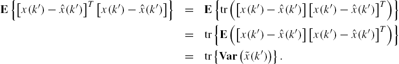
These observations mean that the covariance matrix ![]() of the estimation error is closely related to both some statistics adopted in attack detections/identifications and the estimation accuracy measured by the mathematical expectation of squared estimation errors.
of the estimation error is closely related to both some statistics adopted in attack detections/identifications and the estimation accuracy measured by the mathematical expectation of squared estimation errors.
11.6.2 Sensor Placements
In both attack detections and attack identifications, it is essential to distinguish an abnormal situation of a networked system from its normal situation as fast as possible. This means that it is preferable to have sensors in positions that can make a detector achieve the minimal value of a metric on its residual signal when there do not exist any attacks in the associated networked system and reach a value of that metric as large as possible if the associated networked system has been attacked. Keeping in mind relations among state observers and detectors, in this subsection, we investigate sensor placements with the objective of minimizing state estimation errors.
For this purpose, we adopt the following assumption for the system described by Eqs. (11.69) and (11.70) to reflect characteristics in optimizations of sensor locations.
Assumption 11.1
The matrix ![]() is time invariant. Moreover, each of its rows has a nonzero element equal to 1. Furthermore, each of its columns has at most one nonzero element.
is time invariant. Moreover, each of its rows has a nonzero element equal to 1. Furthermore, each of its columns has at most one nonzero element.
This assumption reflects that all sensor positions have been fixed, each sensor only directly measures one of the states of the networked system, and if a state in the networked system is directly measured, then it can only be measured by one sensor. Under such an assumption, we can directly prove that the number of the sensors in the networked system is equal to the number of nonzero elements in the matrix C, which is an abbreviation of the matrix ![]() when Assumption 11.1 is satisfied.
when Assumption 11.1 is satisfied.
Define the set
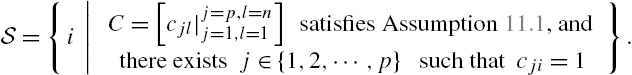
It is clear that this set indicates all the states in the networked system described by Eqs. (11.69) and (11.70) for which there is a sensor measuring its value. With a little abuse of terminology, in this subsection, we call this set the sensor set for that networked system.
For an arbitrary ![]() -dimensional matrix Ξ, let
-dimensional matrix Ξ, let ![]() represent its ith row jth column element,
represent its ith row jth column element, ![]() and
and ![]() . Define scalars
. Define scalars ![]() ,
, ![]() ,
, ![]() , and
, and ![]() respectively as
respectively as

On the basis of the results given in the previous subsection on the Kalman filtering, the following results have been obtained in [15], which establish some relations among the number of sensors, data length, and state estimation accuracy in a networked system.
Theorem 11.6

This theorem reveals that the lower bound of state estimation accuracy decreases only inversely proportionally to the number of the sensors in the system and increases linearly with the increment of the number of the states in the system. This means that estimation errors cannot be significantly reduced through only adding sensors to the system, and for a large-scale system, measurements with a short data length cannot lead to an acceptable estimation accuracy in general.
From this theorem conditions can be derived on the number of sensors and data length required to meet some prescribed estimation accuracy. More precisely, assume that it is required that ![]() with some prescribed positive number α. Then the following conclusions can be derived from Theorem 11.6.
with some prescribed positive number α. Then the following conclusions can be derived from Theorem 11.6.
- • Assume that the date length k is fixed. Then, to satisfy
 , it is necessary that
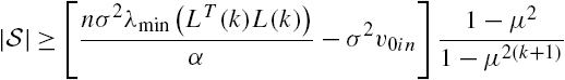
- • Assume that the number of sensors
 , is fixed. Then, to satisfy
 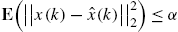 , it is necessary that
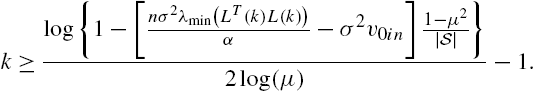
These relations imply that the required number of sensors increases linearly with the increment of the number of the system states, but the required data length increases only logarithmically.
Now, we investigate relations between sensor sets and the covariance matrix of estimation errors, that is, ![]() . For this purpose, define
. For this purpose, define ![]() with
with ![]() as
as ![]() . Then from the definitions of the matrices
. Then from the definitions of the matrices ![]() and
and ![]() it is obvious that
it is obvious that
Let ![]() denote the jth canonical basis of the n-dimensional Euclidean space
denote the jth canonical basis of the n-dimensional Euclidean space ![]() ,
, ![]() , that is,
, that is, ![]() is an n-dimensional column vector with its jth row element 1 and all other elements 0. Moreover, for each
is an n-dimensional column vector with its jth row element 1 and all other elements 0. Moreover, for each ![]() , define the matrix
, define the matrix
Furthermore, let ![]() with
with ![]() , be the indicator function defined as
, be the indicator function defined as

By Assumption 11.1 the output matrix C of the networked system described by Eqs. (11.69) and (11.70) can be expressed as
where ![]() is the position of the nonzero element in the ith row of the matrix C,
is the position of the nonzero element in the ith row of the matrix C, ![]() . Moreover, the following equalities are valid:
. Moreover, the following equalities are valid:
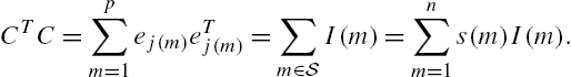
To clarify dependence of the matrices ![]() and
and ![]() on the sensor set
on the sensor set ![]() , we further reexpress them respectively as
, we further reexpress them respectively as ![]() and
and ![]() , where the sensor set
, where the sensor set ![]() is explicitly included. By Eqs. (11.83), (11.84), and (11.85) we have that
is explicitly included. By Eqs. (11.83), (11.84), and (11.85) we have that

where
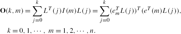
From its definition it is clear that for all ![]() and
and ![]() , the matrix
, the matrix ![]() is independent of either the number of sensors in the system or the positions of the sensors. In addition, this matrix is at least semipositive definite.
is independent of either the number of sensors in the system or the positions of the sensors. In addition, this matrix is at least semipositive definite.
Now, assume that there are two sensor sets ![]() and
and ![]() satisfying
satisfying
Then by Eq. (11.86) the following inequality is immediate:
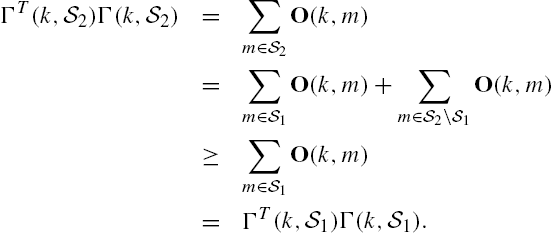
We can therefore declare from Lemma 2.1 that

By Eqs. (11.78) and (11.88) and by Lemma 2.1 we further have that
Eqs. (11.89) and (11.81) mean that, with the addition of some sensors, both the mean squares estimation errors of the Kalman filter and the covariance matrix of its estimation errors monotonically decrease. This is consistent with engineering intuition, as a sensor addition results in more measurement data, which provide more information about the plant state vector and therefore lead to a more accurate state estimate.
However, when the number of sensors is fixed, it is still not very easy to find the optimal sensor positions that minimize either the mean squares estimation errors or the covariance matrix of the state estimation errors [15,20,21].
On the other hand, discussions in the previous section show that observability of a networked system is necessary for the existence of a residual filter that is able to detect/identify an attack. It can be shown, however, that even the problem of finding the best sensor positions that lead to an observable networked system is NP-hard.
In particular, similarly to the proof of Theorem 3.2, we can also show that to recover the state vectors of the networked system described by Eqs. (11.69) and (11.70) from its output measurements ![]() , it is necessary and sufficient that the following matrix
, it is necessary and sufficient that the following matrix ![]() w is of full column rank:
w is of full column rank:

Note that the matrix ![]() is of full column rank if and only if the matrix
is of full column rank if and only if the matrix ![]() is of full rank. In fact, the ranks of these two matrices equal each other [27,28]. When sensor positions are selected to guarantee the observability of a networked system, it is reasonable from these observations to investigate the problem of maximizing the rank of the matrix
is of full rank. In fact, the ranks of these two matrices equal each other [27,28]. When sensor positions are selected to guarantee the observability of a networked system, it is reasonable from these observations to investigate the problem of maximizing the rank of the matrix ![]() under the restrictions that
under the restrictions that ![]() and
and ![]() .
.
Concerning the set function involved in this optimization problem, the following conclusions are obtained.
Theorem 11.7
Assume that the dynamics of a networked system is described by Eqs. (11.69) and (11.70). Moreover, assume that Assumption 11.1 is satisfied by its output matrix ![]() . Define the set function
. Define the set function ![]() as
as
where ![]() . Then this set function is submodular and increasing for each
. Then this set function is submodular and increasing for each ![]() .
.
The proof of this theorem is deferred to the appendix of this chapter.
From this theorem and the results on optimization of the set function given in Chapter 2 we can declare that optimal sensor placements for maximizing the rank of the observability matrix ![]() are in general NP-hard. On the other hand, the greedy heuristic method of that chapter usually gives a good approximation result. But it is worth noting that when the scale of a networked system is large, some computation issues may still arise for this greedy heuristic method, noting that in this case, the matrix
are in general NP-hard. On the other hand, the greedy heuristic method of that chapter usually gives a good approximation result. But it is worth noting that when the scale of a networked system is large, some computation issues may still arise for this greedy heuristic method, noting that in this case, the matrix ![]() of Eq. (11.A.1) often has a high dimension. These are different significantly by the results of Chapter 3, given by Corollary 3.1 and Theorem 3.10. The output matrix there is allowed to take an arbitrary real value for a networked system, and an explicit parameterization is given for all output matrices that lead to an observable system.
of Eq. (11.A.1) often has a high dimension. These are different significantly by the results of Chapter 3, given by Corollary 3.1 and Theorem 3.10. The output matrix there is allowed to take an arbitrary real value for a networked system, and an explicit parameterization is given for all output matrices that lead to an observable system.
When the state transition matrix of the networked system described by Eqs. (11.69) and (11.70) is also time invariant, arguments similar to those of Chapter 3 show that when the observability matrix ![]() is involved in an optimization problem, it is sufficient to only consider the case
is involved in an optimization problem, it is sufficient to only consider the case ![]() .
.
11.6.3 Actuator Placements
In the previous sections, it has been argued that an attacker usually intends to give destructive damages to a system in a stealthy way with small efforts. In this subsection, we investigate selection of input positions for the system described by Eqs. (11.69) and (11.70) such that some metrics on the input efforts can be minimized. For this purpose, we further adopt the following assumption, which is in a dual form of Assumption 11.1 adopted in the previous subsection for studying sensor placements.
Assumption 11.2
The matrix ![]() is time invariant. Moreover, each of its columns has a nonzero element 1. Furthermore, each of its rows has at most one nonzero element.
is time invariant. Moreover, each of its columns has a nonzero element 1. Furthermore, each of its rows has at most one nonzero element.
When this assumption is satisfied, the input matrix ![]() is abbreviated as B for simplicity.
is abbreviated as B for simplicity.
Concerning the system described by Eqs. (11.69) and (11.70), its controllability Gramian at the time instant k, denoted ![]() , is defined as
, is defined as

where ![]() . Note that inputs to a system are usually energy restricted. Moreover, some functions of the controllability Gramian
. Note that inputs to a system are usually energy restricted. Moreover, some functions of the controllability Gramian ![]() have been argued to be nice quantities for measuring energies required to maneuver the system state vector from the zero-valued initial conditions to a prescribed value in the time interval
have been argued to be nice quantities for measuring energies required to maneuver the system state vector from the zero-valued initial conditions to a prescribed value in the time interval ![]() . Depending on whether the average energy required to maneuver the system state vector, a worst-case energy required to maneuver the system state vector or the volume of the states that can be reached through one unit or less of input energies,
. Depending on whether the average energy required to maneuver the system state vector, a worst-case energy required to maneuver the system state vector or the volume of the states that can be reached through one unit or less of input energies, ![]() ,
, ![]() and
and ![]() are utilized respectively [16,17].
are utilized respectively [16,17].
For each ![]() , let
, let ![]() with
with ![]() , be an indicator function defined as
, be an indicator function defined as

By Assumption 11.2 the input matrix B of the networked system can be expressed as
where ![]() is the position of the nonzero element in the ith column of the input matrix B,
is the position of the nonzero element in the ith column of the input matrix B, ![]() . Moreover, similarly to Eq. (11.85), we can obtain the following relation:
. Moreover, similarly to Eq. (11.85), we can obtain the following relation:

where the matrix ![]() is defined as that in the previous subsection.
is defined as that in the previous subsection.
Define the set
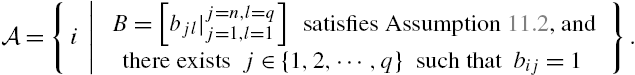
Then it is clear that this set indicates all the states in the networked system described by Eqs. (11.69) and (11.70) that are directly controlled by an actuator. Similarly to the sensor set ![]() , in this subsection, we call this set the actuator set for that networked system.
, in this subsection, we call this set the actuator set for that networked system.
To clarify dependence of the controllability Gramian ![]() on the actuator set
on the actuator set ![]() , we further reexpress it as
, we further reexpress it as ![]() , so that the sensor set
, so that the sensor set ![]() is explicitly included. Using completely the same arguments as those in the derivation of Eq. (11.86), from Eqs. (11.91) and (11.93) we obtain the following relation:
is explicitly included. Using completely the same arguments as those in the derivation of Eq. (11.86), from Eqs. (11.91) and (11.93) we obtain the following relation:

where
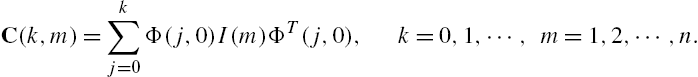
It is clear from its definition that, for all ![]() and
and ![]() , the matrix
, the matrix ![]() is independent of either the number of actuators in the system or the positions of the actuators. In addition, this matrix is at least semipositive definite.
is independent of either the number of actuators in the system or the positions of the actuators. In addition, this matrix is at least semipositive definite.
Now, assume that there are two actuator sets ![]() and
and ![]() satisfying
satisfying
Then by Eq. (11.94) we can obtain the following inequality by the same arguments as those in the derivation of Eq. (11.87):
We can therefore declare from Lemma 2.1 that when both matrices ![]() and
and ![]() are invertible, the following inequalities are valid:
are invertible, the following inequalities are valid:
that is, through adding some other actuators, both the average energy required to maneuver the system state vector and the worst-case energy required to maneuver the system state vector decrease monotonically, whereas the volume of the states that can be reached through one unit or less of input energies increases monotonically. Once again, this is in a good agreement with engineering intuition.
However, optimization of these metrics is generally mathematically difficult. In particular, we have the following results.
Theorem 11.8
Proof
From Eq. (11.98) we can directly declare that this function is increasing.
To prove its submodularity, assume that ξ is an arbitrary element of the set ![]() . Moreover, assume that
. Moreover, assume that ![]() and
and ![]() are two sets satisfying
are two sets satisfying ![]() . Define the matrix
. Define the matrix ![]() and the function
and the function ![]() respectively as
respectively as

where ![]() .
.
By Eq. (11.95) we have that
On the other hand, noting that by its definition the matrix ![]() is at least positive semidefinite, it is obvious that
is at least positive semidefinite, it is obvious that
We can therefore declare from Lemma 2.1 that
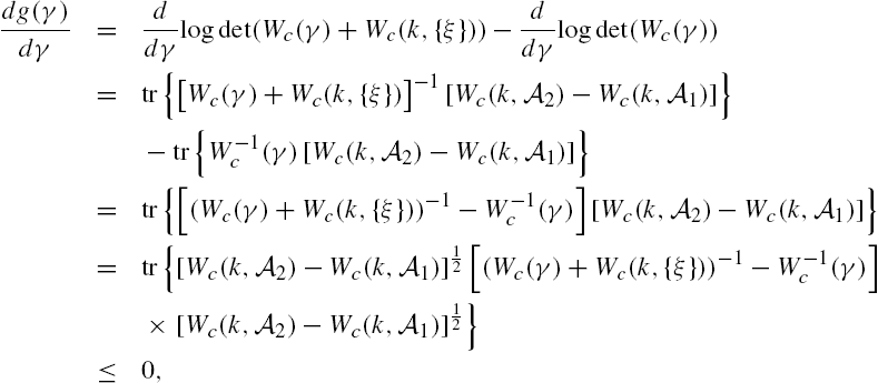
which implies that ![]() .2
.2
On the other hand, from the definition of the function ![]() it is obvious that
it is obvious that
Note that from Eq. (11.94) we immediately have that
for all ![]() and
and ![]() . Hence we can claim that
. Hence we can claim that ![]() and
and ![]() are in fact equal to the values of the following set function
are in fact equal to the values of the following set function ![]() respectively at
respectively at ![]() and
and ![]() :
:
The proof can now be completed by an application of Lemma 2.8. □
In addition to the set function ![]() , it has also been proven in [16,17] that some other set functions, such as
, it has also been proven in [16,17] that some other set functions, such as ![]() ,
, ![]() , etc., are also monotone increasing and submodular. This means that maximization of these set functions is in general NP-hard, but the greedy heuristic algorithm described in Chapter 2 usually works well approximately. Once again, as in the sensor placement problem, computation issues may arise for a large-scale system in the application of that greedy heuristic algorithm, noting that the associated matrix in this case still has a great dimension, which is not very convenient for numerical computations.
, etc., are also monotone increasing and submodular. This means that maximization of these set functions is in general NP-hard, but the greedy heuristic algorithm described in Chapter 2 usually works well approximately. Once again, as in the sensor placement problem, computation issues may arise for a large-scale system in the application of that greedy heuristic algorithm, noting that the associated matrix in this case still has a great dimension, which is not very convenient for numerical computations.
On the other hand, from the duality between controllability and observability of a system, similiar results can be established for sensor placements using the associated observability Gramian.
In the above investigations on sensor/actuator placements, the output/input matrix of the system is restricted by Assumption 11.1/11.2. The associated results can be extended to a more general situation in which each row of the output matrix can take values from a set of some candidate rows, or each column of the input matrix can take values from a set of some candidate columns. The major required modification in these extensions is a redefinition of the matrix ![]() adopted in the aforementioned investigations. Details can be found in the related literature, such as [16,17] and the references therein.
adopted in the aforementioned investigations. Details can be found in the related literature, such as [16,17] and the references therein.
11.7 Concluding Remarks
Importance of safety is now widely recognized for a networked system, especially with the ambitious introduction of public communication channels into a control system. In this chapter, we investigated some basic issues in system designs closely related to attack detection and identification, which reveals some relations among attack detectability/identifiability, system controllability/observability, and actuator/sensor placement. To develop an algorithm applicable to actual engineering problems, some other factors, such as robustness against modeling errors, stochastic properties of external disturbances, and measurement errors, must also be taken into account.
11.8 Bibliographic Notes
Network safety has been extensively investigated in power systems. [6] summarizes various important aspects of this problem and some interesting recent advancements. Recent interest in this problem are mainly stimulated by the prospective introduction of public communication channels into control systems, which brings some new characteristics into this field. Many essential issues are still in their primary stages toward a complete settlement. [2,7] are some recent surveys about this problem.
Basic concepts and results for combinatorial optimizations can be found in [26,30]. Concerning with convex optimization, [25,31] provides an excellent introduction on its essential motivations and results.
The notion of a system matrix is due to Rosenbrock, who also introduced zeros of linear multivariable systems in terms of the Smith–McMillan form of the system transfer matrix in [10,13]. The concept of weakly unobservable subspace appears to be firstly introduced for a discrete-time system by Silverman [32]. A summary and some detailed discussions can be found in [11]. Connections between the spectral properties of a weakly unobservable subspace and the system zeros are also dealt with in [33], and [34] has studied connections between the system zeros and the state space geometric structure of the system.
Appendix 11.A
11.A.1 Proof of Theorem 11.7
From the definition of the matrix ![]() and Eq. (11.85) it is obvious that
and Eq. (11.85) it is obvious that

where

It is clear that, for each ![]() , the matrix
, the matrix ![]() is at least positive semidefinite. Hence, for arbitrary sensor sets
is at least positive semidefinite. Hence, for arbitrary sensor sets ![]() and
and ![]() satisfying
satisfying ![]() , the following relations are valid:
, the following relations are valid:

Let ![]() denote the ith eigenvalue of an
denote the ith eigenvalue of an ![]() -dimensional symmetric matrix that satisfies
-dimensional symmetric matrix that satisfies ![]() . By Lemma 2.1 and the last equation we have that, for each
. By Lemma 2.1 and the last equation we have that, for each ![]() ,
,
Note that, for a positive semidefinite matrix, its rank is equal to the number of its nonzero eigenvalues. Moreover, each of its eigenvalues is not smaller than 0. We can therefore declare from Eq. (11.A.3) that
that is, the set function ![]() of Eq. (11.90) is increasing.
of Eq. (11.90) is increasing.
To prove its submodularity, define the derived set function ![]() for each
for each ![]() as
as
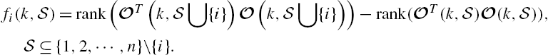
Note that, for arbitrary ![]() -dimensional real matrices X and Y,
-dimensional real matrices X and Y,
where ![]() stands for the dimension of a subspace [27,28]. From this property, the definition of the set function
stands for the dimension of a subspace [27,28]. From this property, the definition of the set function ![]() , and from Eq. (11.A.1) we have that
, and from Eq. (11.A.1) we have that

Assume now that ![]() . Then from the relation
. Then from the relation
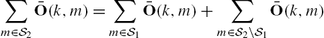
and the definition of the matrix ![]() ,
, ![]() , the following relation can be established by some algebraic manipulations:
, the following relation can be established by some algebraic manipulations:
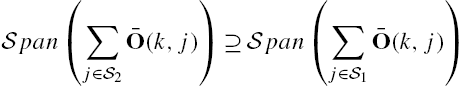
Therefore

which further leads the following inequality:

Substituting this inequality into Eq. (11.A.6), we have that, under the condition that ![]() and
and ![]() , the following inequality is true:
, the following inequality is true:
that is, this derived set function is decreasing.
We can therefore declare from Lemma 2.8 that the set function ![]() is submodular. This completes the proof. □
is submodular. This completes the proof. □