Chapter 1. Design and implement database objects

Developing and implementing a database for SQL Server starts with understanding both the process of designing a database and the basic structures that make up a database. A firm grip on those fundamentals is a must for an SQL Server developer, and is even more important for taking this exam.

We begin with the fundamentals of a typical database meant to store information about a business. This is generally referred to as online transaction processing (OLTP), where the goal is to store data that accurately reflects what happens in the business in a manner that works well for the applications. For this pattern, we review the relational database design pattern, which is covered in Skill 1.1. OLTP databases can be used to store more than business transactions, including the ability to store any data about your business, such as customer details, appointments, and so on.

Skills 1.2 and 1.3 cover some of the basic constructs, including indexes and views, that go into forming the physical database structures (Transact-SQL code) that applications use to create the foundational objects your applications use to do business.

In Skill 1.4 we explore columnstore indexes that focus strictly on analytics. While discussing analytics, we look at the de facto standard for building reporting structures called dimensional design. In dimensional design, the goal is to format the data in a form that makes it easier to extract results from large sets of data without touching a lot of different structures.

Skills in this chapter:

Design and implement a relational database schema

Design and implement indexes

Design and implement views

Implement columnstore indexes

Most of the examples in this book, and likely on the exam, are abstract, contrived, and targeted to a single example; either using a sample database from Microsoft, or using examples that include only the minimal details for the particular concept being reviewed. There are, however, a few topics that require a more detailed narrative. To review the topic of designing a database, we need to start out with some basic requirements, using them to design a database that demonstrates database design concepts and normalization.

We have a scenario that defines a database need, including some very basic requirements. Questions on the exam can easily follow this pattern of giving you a small set of requirements and table structures that you need to match to the requirements. This scenario will be used as the basis for the first two sections of this chapter.

Imagine that you are trying to write a system to manage an inventory of computers and computer peripherals for a large organization. Someone has created a document similar in scope to the following scenario (realistic requirements are often hundreds or even thousands of pages long, but you can learn a lot from a single paragraph):

We have 1,000 computers, comprised of laptops, workstations, and tablets. Each computer has items associated with it, which we will list as mouse, keyboard, etc. Each computer has a tag number associated with it, and is tagged on each device with a tag graphic that can be read by tag readers manufactured by “Trey Research” (http://www.treyresearch.net/) or “Litware, Inc” (http://www.litwareinc.com/). Of course tag numbers are unique across tag readers. We don’t know which employees are assigned which computers, but all computers that cost more than $300 are inventoried for the first three years after purchase using a different software system. Finally, employees need to have their names recorded, along with their employee number in this system.

Let’s look for the tables and columns that match the needs of the requirements. We won’t actually create any tables yet, because this is just the first step in the process of database design. In the next section, we spend time looking at specific tests that we apply to our design, followed by two sections on creating the table structures of a database.

The process of database design involves scanning requirements, looking for key types of words and phrases. For tables, you look for the nouns such as “computers” or “employee.” These can be tables in your final database. Some of these nouns you discover in the requirements are simply subsets of one another: “computer” and “laptop.” For example, laptop is not necessarily its own table at all, but instead may be just a type of computer. Whether or not you need a specific table for laptops, workstations, or tablets isn’t likely to be important. The point is to match a possible solution with a set of requirements.

After scanning for nouns, you have your list of likely objects on which to save data. These will typically become tables after we complete our design, but still need to be refined by the normalization process that we will cover in the next section:

1. Computer

2. Employee

The next step is to look for attributes of each object. You do this by scanning the text looking for bits of information that might be stored about each object. For the Computer object, you see that there is a Type of Computer (laptop, workstation, or tablet), an Associated Item List, a Tag, a Tag Company, and a Tag Company URL, along with the Cost of the computer and employee that the computer is assigned to. Additionally, in the requirements, we also have the fact that they keep the computer inventoried for the first three years after purchase if it is > $300, so we need to record the Purchase Date. For the Employee object we are required to capture their Name and Employee Number.

Now we have the basic table structures to extract from the requirements, (though we still require some refinement in the following section on normalization) and we also define schemas, which are security/organizational groupings of tables and code for our implemented database. In our case, we define two schemas: Equipment and HumanResources.

Our design consists of the following possible tables and columns:

1. Equipment.Computer: (ComputerType, AssociatedItemList, Tag, TagCompany, TagCompanyURL, ComputerCost, PurchaseDate, AssignedEmployee)

2. HumanResources.Employee: (Name, EmployeeNumber)

The next step in the process is to look for how you would uniquely identify a row in your potential database. For example, how do you tell one computer from another. In the requirements, we are told that, “Each computer has a tag number,” so we will identify that the Tag attribute must be unique for each Computer.

This process of designing the database requires you to work through the requirements until you have a set of tables that match the requirements you’ve been given.

In the real world, you don’t alter the design from the provided requirements unless you discuss it with the customer. And in an exam question, you do whatever is written, regardless of whether it makes perfect sense. Do you need the URL of the TagCompany, for instance? If so, why? For the purposes of this exam, we will focus on the process of translating words into tables.

The typical approach in database design is to work instinctively and then use the principles of normalization as a test to your design. You can expect questions on normalization to be similar, asking questions like, “is this a well-designed table to meet some requirement?” and any of the normal forms that might apply.

However, in this section, we review the normal forms individually, just to make the review process more straightforward. The rules are stated in terms of forms, some of which are numbered, and some which are named for the creators of the rule. The rules form a progression, with each rule becoming more and more strict. To be in a stricter normal form, you need to also conform to the lesser form, though none of these rules are ever followed one hundred percent of the time.

The most important thing to understand will be the concepts of normalization, and particularly how to verify that a design is normalized. In the following sections, we will review two families of normalization concepts:

Rules covering the shape of a table

Rules covering the relationship of non-key attributes to key attributes

The first part of these rules is defined by the mathematical definition of a relation (which is more or less synonymous with the proper structure of a table). Relations require that you have no duplicated rows. In database terminology, a column or set of columns that are used to uniquely identify one row from another is called a key. There are several types of keys we discuss in the following section, and they are all columns to identify a row (other than what is called a foreign key, which are columns in a table that reference another table’s key attributes). Continuing with the example we started in the previous section, we have one such example in our design so far with: HumanResources.Employee: (Name, EmployeeNumber).

Using the Employee table definition that we started with back in the first section of this chapter, it would be allowable to have the following two rows of data represented:

Click here to view code image

Name                              EmployeeNumber
--------------------------------- ---------------
Harmetz, Adam                     000010012
Harmetz, Adam                     000010012

This would not be a proper table, since you cannot tell one row from another. Many people try to fix this by adding some random bit of data (commonly called an artificial key value), like some auto generated number. This then provides a structure with data like the following, with some more data that is even more messed up, but still legal as the structure allows:

Click here to view code image

EmployeeId Name                            EmployeeNumber
----------- ------------------------------ ------------------------
          1 Harmetz, Adam                  000010012
          2 Harmetz, Adam                  000010012
          3 Popkova, Darya                 000000012
          4 Popkova, Darya                 000000013

In the next section on creating tables, we begin the review of ways we can enforce the uniqueness on data in column(s), but for now, let’s keep it strictly in design mode. While this seems to make the table better, unless the EmployeeId column actually has some meaning to the user, all that has been done is to make the problem worse because someone looking for Adam’s information can get one row or the other. What we really want is some sort of data in the table that makes the data unique based on data the user chooses. Name is not the correct choice, because two people can have the same name, but EmployeeNumber is data that the user knows, and is used in an organization to identify an employee. A key like this is commonly known as a natural key. When your table is created, the artificial key is referred to as a surrogate key, which means it is a stand-in for the natural key for performance reasons. We talk more about these concepts in the “Determining the most efficient data types to use” section and again in Chapter 2, Skill 2.1 when choosing UNIQUE and PRIMARY KEY constraints.

After defining that EmployeeNumber must be unique, our table of data looks like the following:

Click here to view code image

EmployeeId Name                              EmployeeNumber
---------- --------------------------------- ----------------------
         1 Harmetz, Adam                     000010012
         2 Popkova, Darya                    000000013

The next two criteria concerning row shape are defined in the First Normal Form. It has two primary requirements that your table design must adhere to:

1. All columns must be atomic—that is, each column should represent one value

2. All rows of a table must contain the same number of values—no arrays

Starting with atomic column values, consider that we have a column in the Employee table we are working on that probably has a non-atomic value (probably because it is based on the requirements). Be sure to read the questions carefully to make sure you are not assuming things. The name column has values that contain a delimiter between what turns out to be the last name and first name of the person. If this is always the case then you need to record the first and last name of the person seperately. So in our table design, we will break ‘Harmetz, Adam’ into first name: ‘Adam’ and last name: ‘Harmetz’. This is represented here:

Click here to view code image

EmployeeId LastName        FirstName         EmployeeNumber
---------- --------------- ----------------- ---------------
         1 Harmetz         Adam              000010012
         2 Popkova         Darya             000000013

For our design, let’s leave off the EmployeeId column for clarity in the design. So the structure looks like:

Click here to view code image

HumanResources.Employee (EmployeeNumber [key], LastName, FirstName)

Obviously the value here is that when you need to search for someone named ‘Adam,’ you don’t need to search on a partial value. Queries on partial values, particularly when the partial value does not include the leftmost character of a string, are not ideal for SQL Server’s indexing strategies. So, the desire is that every column represents just a single value. In reality, names are always more complex than just last name and first name, because people have suffixes and titles that they really want to see beside their name (for example, if it was Dr. Darya Popkova, feelings could be hurt if the Dr. was dropped in correspondence with them.)

The second criteria for the first normal form is the rule about no repeating groups/arrays. A lot of times, the data that doesn’t fit the atomic criteria is not different items, such as parts of a name, but rather it’s a list of items that are the same types of things. For example, in our requirements, there is a column in the Computer table that is a list of items named AssociatedItemList and the example: ‘mouse, keyboard.’ Looking at this data, a row might look like the following:

Click here to view code image

Tag    AssociatedItemList
------ ------------------------------------
 s344  mouse, keyboard

From here, there are a few choices. If there are always two items associated to a computer, you might add a column for the first item, and again for a second item to the structure. But that is not what we are told in the requirements. They state: “Each computer has items associated with it.” This can be any number of items. Since the goal is to make sure that column values are atomic, we definitely want to get rid of the column containing the delimited list. So the next inclination is to make a repeating group of column values, like:

Click here to view code image

Tag    AssociatedItem1 AssociatedItem2 ... AssociatedItemN
------ --------------- --------------- ... -----------------
 s344  mouse           keyboard        ... not applicable

This however, is not the desired outcome, because now you have created a fixed array of associated items with an index in the column name. It is very inflexible, and is limited to the number of columns you want to add. Even worse is that if you need to add something like a tag to the associated items, you end up with a structure that is very complex to work with:

Click here to view code image

Tag    AssociatedItem1 AssociatedItem1Tag AssociatedItem2 AssociatedItem2Tag
------ --------------- ------------------ --------------- ---------------------
  s344 mouse           r232               keyboard        q472

Instead of this structure, create a new table that has a reference back to the original table, and the attributes that are desired:

Tag    AssociatedItem
------ -----------------
  s344 mouse
  s344 keyboard

So our object is: Equipment.ComputerAssociatedItem (Tag [Reference to Computer], AssociatedItem, [key Tag, AssociatedItem).

Now, if you need to search for computers that have keyboards associated, you don’t need to either pick it out of a comma delimited list, nor do you need to look in multiple columns. Assuming you are reviewing for this exam, and already know a good deal about how indexes and queries work, you should see that everything we have done in this first section on normalization is going to be great for performance. The entire desire is to make scalar values that index well and can be searched for. It is never wrong to do a partial value search (if you can’t remember how keyboard is spelled, for example, looking for associated items LIKE ‘%k%’ isn’t a violation of any moral laws, it just isn’t a design goal that you are be trying to attain.

Click here to view code image

HumanResources.Employee (EmployeeNumber)

Equipment.Computer (Tag)

In this section, we are going to look at how the other columns in the table relate to the key attributes. There are three normal forms that are related to this discussion:

Second Normal Form All attributes must be a fact about the entire primary key and not a subset of the primary key.

Third Normal Form All attributes must be a fact about the entire primary key, and not any non-primary key attributes

For the second normal form to be a concern, you must have a table with multiple columns in the primary key. For example, say you have a table that defines a car parked in a parking space. This table can have the following columns:

CarLicenseTag (Key Column1)

SpaceNumber (Key Column2)

ParkedTime

CarColor

CarModel

CarManufacturer

CarManufacturerHeadquarters

Each of the nonkey attributes should say something about the combination of the two key attributes. The ParkedTime column is the time when the car was parked. This attribute makes sense. The others are all specifically about the car itself. So you need another table that looks like the following where all of the columns are moved to (the CarLicenseTag column stays as a reference to this new table. Now you have a table that represents the details about a car with the following columns:

CarLicenseTag (Key Column)

CarColor

CarModel

CarManufacturer

CarManufacturerHeadquarters

Since there is a single key column, this must be in second normal form (like how the table we left behind with the CarLicenseTag, SpaceNumber and ParkedTime since ParkedTime references the entire key.) Now we turn our attention to the third normal form. Here we make sure that each attribute is solely focused on the primary key column. A car has a color, a model, and a manufacturer. But does it have a CarManufacturerHeadquarters? No, the manufacturer does. So you would create another table for that attribute and the key CarManufacturer. Progress through the design making more tables until you have eliminated redundancy.

The redundancy is troublesome because if you were to change the headquarter location for a manufacturer, you might need to do so for more than the one row or end up with mismatched data. Raymond Boyce and Edgar Codd (the original author of the normalization forms), refined these two normal forms into the following normal form, named after them:

Boyce-Codd Normal Form Every candidate key is identified, all attributes are fully dependent on a key, and all columns must identify a fact about a key and nothing but a key.

All of these forms are stating that once you have set what columns uniquely define a row in a table, the rest of the columns should refer to what the key value represents. Continuing with the design based on the scenario/requirement we have used so far in the chapter, consider the Equipment.Computer table. We have the following columns defined (Note that AssociatedItemList was removed from the table in the previous section):

Click here to view code image

Tag (key attribute), ComputerType, TagCompany, TagCompanyURL, ComputerCost,
PurchaseDate, AssignedEmployee

In this list of columns for the Computer table, your job is to decide which of these columns describes what the Tag attribute is identifying, which is a computer. The Tag column value itself does not seem to describe the computer, and that’s fine. It is a number that has been associated with a computer by the business in order to be able to tell two physical devices apart. However, for each of the other attributes, it’s important to decide if the attribute describes something about the computer, or something else entirely. It is a good idea to take each column independently and think about what it means.

ComputerType Describes the type of computer that is being inventoried.

TagCompany The tag has a tag company, and since we defined that the tag number was unique across companies, this attribute is violating the Boyce-Codd Normal Form and must be moved to a different table.

TagCompanyURL Much like TagCompany, the URL for the company is definitely not describing the computer.

ComputerCost Describes how much the computer cost when purchased.

PurchaseDate Indicates when the computer was purchased.

AssignedEmployee This is a reference to the Employee structure. So while a computer doesn’t really have an assigned employee in the real world, it does make sense in the overall design as it describes an attribute of the computer as it stands in the business.

Now, our design for these two tables looks like the following:

Click here to view code image

Equipment.Computer (Tag [key, ref to Tag], ComputerType, ComputerCost, PurchaseDate,
AssignedEmployee [Reference to Employee]

Equipment.Tag (Tag [key], TagCompany, TagCompanyURL)

If the tables have the same key columns, do we need two tables? This depends on your requirements, but it is not out of the ordinary that you have two tables that are related to one another with a cardinality of one-to-one. In this case, you have a pool of tags that get created, and then assigned, to a device, or tags could have more than one use. Make sure to always take your time and understand the requirements that you are given with your question.

So we now have:

Click here to view code image

Equipment.Computer (Tag [key, Ref to Tag], ComputerType, ComputerCost, PurchaseDate,
AssignedEmployee [Reference to Employee]
Equipment.TagCompany (TagCompany [key], TagCompanyURL)
Equipment.Tag (Tag [key], TagCompany [Reference to TagCompany])

And we have this, in addition to the objects we previously specified:

Click here to view code image

Equipment.ComputerAssociatedItem (Tag [Reference to Computer], AssociatedItem, [key
Tag, AssociatedItem)

HumanResources.Employee (EmployeeNumber [key], LastName, FirstName)

Generally speaking, the third normal form is referred to as the most important normal form, and for the exam it is important to understand that each table has one meaning, and each scalar attribute refers to the entire natural key of the final objects. Good practice can be had by working through tables in your own databases, or in our examples, such as the WideWorldImporters (the newest example database they have created), AdventureWorks, Northwind, or even Pubs. None of these databases are perfect, because doing an excellent job designing a database sometimes makes for really complex examples. Note that we don’t have the detailed requirements for these sample databases. Don’t be tricked by thinking you know what a system should look like by experience. The only thing worse than having no knowledge of your customer’s business is having too much knowledge of their business.

One last term needs to be defined: denormalization. After you have normalized your database, and have tested it out, there can be reasons to undo some of the things you have done for performance. For example, later in the chapter, we add a formatted version of an employee’s name. To do this, it duplicates the data in the LastName and FirstName columns of the table (in order to show a few concepts in implementation). A poor design for this is to have another column that the user can edit, because they might not get the name right. Better implementations are available in the implementation of a database.

Before we move onto CREATE TABLE statements, a brief discussion on object naming is useful. You sometimes see names like the following used to name a table that contain rows of purchase orders:

PurchaseOrder

PURCHASEORDER

PO

purchase_orders

tbl_PurchaseOrder

A12

[Purchase Order] or “Purchase Order”

Of these naming styles, there are a few that are typically considered sub-optimal:

PO Using abbreviations, unless universally acceptable tend to make a design more complex for newcomers and long-term users alike.

PURCHASEORDER All capitals tends to make your design like it is 1970, which can hide some of your great work to make a modern computer system.

tbl_PurchaseOrder Using a clunky prefix to say that this is a table reduces the documentation value of the name by making users ask what tbl means (admittedly this could show up in exam questions as it is not universally disliked).

A12 This indicates that this is a database where the designer is trying to hide the details of the database from the user.

[Purchase Order] or “Purchase Order” Names that require delimiters, [brackets], or “double-quotes” are terribly hard to work with. Of the delimiter types, double-quotes are more standards-oriented, while the brackets are more typical SQL Server coding. Between the delimiters you can use any Unicode characters.

The more normal, programmer friendly naming standards are using Pascal-casing (Leading character capitalized, words concatenated: PurchaseOrder), Camel Casing (leading character lower case: purchaseOrder), or using underscores as delimiters (purchase_order).

Sometimes names are plural, and sometimes singular, and consistency is the general key. For the exam, there are likely to be names of any format, plural, singular, or both. Other than interpreting the meaning of the name, naming is not listed as a skill.

To start with, create a schema to put objects in. Schemas allow you to group together objects for security and logical ordering. By default, there is a schema in every database called dbo, which is there for the database owner. For most example code in this chapter, we use a schema named Examples located in a database named ExamBook762Ch1, which you see referenced in some error messages.

Click here to view code image

CREATE SCHEMA Examples;
GO --CREATE SCHEMA must be the only statement in the batch

The CREATE SCHEMA statement is terminated with a semicolon at the end of the statement. All statements in Transact-SQL can be terminated with a semicolon. While not all statements must end with a semicolon in SQL Server 2016, not terminating statements with a semicolon is a deprecated feature, so it is a good habit to get into. GO is not a statement in Transact-SQL it is a batch separator that splits your queries into multiple server communications, so it does not need (or allow) termination.

To create our first table, start with a simple structure that’s defined to hold the name of a widget, with attributes for name and a code:

Click here to view code image

CREATE TABLE Examples.Widget
(
    WidgetCode  varchar(10) NOT NULL
           CONSTRAINT PKWidget PRIMARY KEY,
    WidgetName  varchar(100) NULL
);

Let’s break down this statement into parts:

Click here to view code image

CREATE TABLE Examples.Widget

Here we are naming the table to be created. The name of the table must be unique from all other object names, including tables, views, constraints, procedures, etc. Note that it is a best practice to reference all objects explicitly by at least their two-part names, which includes the name of the object prefixed with a schema name, so most of the code in this book will use two-part names. In addition, object names that a user may reference directly such as tables, views, stored procedures, etc. have a total of four possible parts. For example, Server.Database.Schema.Object has the following parts:

Server The local server, or a linked server name that has been configured. By default, the local server from which you are executing the query.

Database The database where the object you are addressing resides. By default, this is the database that to which you have set your context.

Schema The name of the schema where the object you are accessing resides within the database. Every login has a default schema which defaults to dbo. If the schema is not specified, the default schema will be searched for a matching name.

Object The name of the object you are accessing, which is not optional.

In the CREATE TABLE statement, if you omit the schema, it is created in the default schema. So the CREATE TABLE Widget would, by default, create the table dbo.Widget in the database of context. You can create the table in a different database by specifying the database name: CREATE TABLE Tempdb..Widget or Tempdb.dbo.Widget. There is an article here: (https://technet.microsoft.com/en-us/library/ms187879.aspx.) from an older version of books online that show you the many different forms of addressing an object.

The next line:

Click here to view code image

    WidgetCode  varchar(10) NOT NULL

This specifies the name of the column, then the data type of that column. There are many different data types, and we examine their use and how to make the best choice in the next section. For now, just leave it as this determines the format of the data that is stored in this column. NOT NULL indicates that you must have a known value for the column. If it simply said NULL, then it indicates the value of the column is allowed to be NULL.

NULL is a special value that mathematically means UKNOWN. A few simple equations that can help clarify NULL is that: UNKNOWN + any value = UNKNOWN, and NOT(UNKNOWN) = UNKNOWN. If you don’t know a value, adding any other value to it is still unknown. And if you don’t know if a value is TRUE or FALSE, the opposite of that is still not known. In comparisons, A NULL expression is never equivalent to a NULL expression. So if you have the following conditional: IF (NULL = NULL); the expression would not be TRUE, so it would not succeed.

If you leave off the NULL specification, whether or not the column allows NULL values is based on a couple of things. If the column is part of a PRIMARY KEY constraint that is being added in the CREATE TABLE statement (like in the next line of code), or the setting: SET ANSI_NULL_DFLT_ON, then NULL values are allowed.

The following line of code is a continuation of the previous line of code, since it was not terminated with a comma (broken out to make it easier to explain):

Click here to view code image

                  CONSTRAINT PKWidget PRIMARY KEY,

This is how you add a constraint to a single column. In this case, we are defining that the WidgetCode column is the only column that makes up the primary key of the table. The CONSTRAINT PKWidget names the constraint. The constraint name must be unique within the schema, just like the table name. If you leave the name off and just code it as PRIMARY KEY, SQL Server provides a name that is guaranteed unique, such as PK__Widget__1E5F7A7F7A139099. Such a name changes every time you create the constraint, so it’s really only suited to temporary tables (named either with # or ## as a prefix for local or global temporary objects, respectively).

Alternatively, this PRIMARY KEY constraint could have been defined independently of the column definition as (with the leading comma there for emphasis):

Click here to view code image

                     ,CONSTRAINT PKWidget PRIMARY KEY (WidgetCode),

This form is needed when you have more than one column in the PRIMARY KEY constraint, like if both the WidgetCode and WidgetName made up the primary key value:

Click here to view code image

                     ,CONSTRAINT PKWidget PRIMARY KEY (WidgetCode, WidgetName),

This covers the simple version of the CREATE TABLE statement, but there are a few additional settings to be aware of. First, if you want to put your table on a file group other than the default one, you use the ON clause:

Click here to view code image

CREATE TABLE Examples.Widget
(
    WidgetCode  varchar(10) NOT NULL
           CONSTRAINT PKWidget PRIMARY KEY,
    WidgetName  varchar(100) NULL
) ON FileGroupName;

There are also table options for using temporal extensions, as well as partitioning. These are not a part of this exam, so we do not cover them in any detail, other than to note their existence.

In addition to being able to use the CREATE TABLE statement to create a table, it is not uncommon to encounter the ALTER TABLE statement on the exam to add or remove a constraint. The ALTER TABLE statement allows you to add columns to a table and make changes to some settings.

For example, you can add a column using:

Click here to view code image

ALTER TABLE Examples.Widget
    ADD NullableColumn int NULL;

If there is data in the table, you either have to create the column to allow NULL values, or create a DEFAULT constraint along with the column (which is covered in greater detail in Chapter 2, Skill 2.1).

Click here to view code image

ALTER TABLE Examples.Widget
    ADD NotNullableColumn int NOT NULL
        CONSTRAINT DFLTWidget_NotNullableColumn DEFAULT ('Some Value');
To drop the column, you need to drop referencing constraints, which you also do with the
ALTER TABLE statement:

ALTER TABLE Examples.Widget
    DROP DFLTWidget_NotNullableColumn;

Finally, we will drop this column (because it would be against the normalization rules we have discussed to have this duplicated data) using:

Click here to view code image

ALTER TABLE Examples.Widget
    DROP COLUMN NotNullableColumn;

It serves as the first limitation of domain of data values that the columns can store. If the range of data desired is the name of the days of the week, having a column that allows only integers is completely useless. If you need the values in a column to be between 0 and 350, a tinyint won’t work because it has a maximum of 256, so a better choice is smallint, that goes between –32,768 and 32,767, In Chapter 2, we look at several techniques using CONSTRAINT and TRIGGER objects to limit a column’s value even further.

It is important for performance Take a value that represents the 12th of July, 1999. You could store it in a char(30) as ‘12th of July, 1999’, or in a char(8) as ‘19990712’. Searching for one value in either case requires knowledge of the format, and doing ranges of date values is complex, and even very costly, performance-wise. Using a date data type makes the coding natural for the developer and the query processor.

When handled improperly, data types are frequently a source of interesting issues for users. Don’t limit data enough, and you end up with incorrect, wildly formatted data. Limit too much, like only allowing 35 letters for a last name, and Janice “Lokelani” Keihanaikukauakahihuliheekahaunaele has to have her name truncated on her driver’s license (true story, as you can see in the following article on USA Today http://www.usatoday.com/story/news/nation/2013/12/30/hawaii-long-name/4256063/).

SQL Server has an extensive set of data types that you can choose from to match almost any need. The following list contains the data types along with notes about storage and purpose where needed.

Precise Numeric Stores number-based data with loss of precision in how it stored.

bit Has a domain of 1, 0, or NULL; Usually used as a pseudo-Boolean by using 1 = True, 0 = False, NULL = Unknown. Note that some typical integer operations, like basic math, cannot be performed. (1 byte for up to 8 values)

tinyint Integers between 0 and 255 (1 byte).

smallint Integers between –32,768 and 32,767 (2 bytes).

int Integers between 2,147,483,648 to 2,147,483,647 (–2^31 to 2^31 – 1) (4 bytes).

bigint Integers between 9,223,372,036,854,775,808 to 9,223,372,036,854,775,807 (-2^63 to 2^63 – 1) (8 bytes).

decimal (or numeric which are functionally the same, with decimal the more standard type): All numbers between –10^38 – 1 and 10^38 – 1, with a fixed set of digits up to 38. decimal(3,2) would be a number between -9.99 and 9.99. And decimal(38,37), with be a number with one digit before the decimal point, and 37 places after it. Uses between 5 and 17 bytes, depending on precision.

money Monetary values from –922,337,203,685,477.5808 through 922,337,203,685,477.5807 (8 bytes).

smallmoney Money values from –214,748.3648 through 214,748.3647 (4 bytes).

Approximate numeric data Stores approximations of numbers based on IEEE 754 standard, typically for scientific usage. Allows a large range of values with a high amount of precision but you lose precision of very large or very small numbers.

float(N) Values in the range from –1.79E + 308 through 1.79E + 308 (storage varies from 4 bytes for N between 1 and 24, and 8 bytes for N between 25 and 53).

real Values in the range from –3.40E + 38 through 3.40E + 38. real is an ISO synonym for a float(24) data type, and hence equivalent (4 bytes).

Date and time values Stores values that deal storing a point in time.

date Date-only values from January 1, 0001, to December 31, 9999 (3 bytes).

time(N) Time-of-day-only values with N representing the fractional parts of a second that can be stored. time(7) is down to HH:MM:SS.0000001 (3 to 5 bytes).

datetime2(N) This type stores a point in time from January 1, 0001, to December 31, 9999, with accuracy just like the time type for seconds (6 to 8 bytes).

datetimeoffset Same as datetime2, plus includes an offset for time zone offset (does not deal with daylight saving time) (8 to 10 bytes).

smalldatetime A point in time from January 1, 1900, through June 6, 2079, with accuracy to 1 minute (4 bytes).

datetime Points in time from January 1, 1753, to December 31, 9999, with accuracy to 3.33 milliseconds (so the series of fractional seconds starts as: .003, .007, .010, .013, .017 and so on) (8 bytes).

Binary data Strings of bits used for storing things like files, encrypted values, etc. Storage for these data types is based on the size of the data stored in bytes, plus any overhead for variable length data.

binary(N) Fixed-length binary data with a maximum value of N of 8000, for an 8,000 byte long binary value.

varbinary(N) Variable-length binary data with maximum value of N of 8,000.

varbinary(max) Variable-length binary data up to (2^31) – 1 bytes (2GB) long. Values are often stored using filestream filegroups, which allow you to access files directly via the Windows API, and directly from the Windows File Explorer using filetables.

Character (or string) data String values, used to store text values. Storage is specified in number of characters in the string.

char(N) Fixed-length character data up to 8,000 characters long. When using fixed length data types, it is best if most of the values in the column are the same, or at least use most of the column.

varchar(N) Variable-length character data up to 8,000 characters long.

varchar(max) Variable-length character data up to (2^31) – 1 bytes (2GB) long. This is a very long string of characters, and should be used with caution as returning rows with 2GB per row can be hard on your network connection.

nchar, nvarchar, nvarchar(max) Unicode equivalents of char, varchar, and varchar(max). Unicode is a double (and in some cases triple) byte character set that allows for more than the 256 characters at a time that the ASCII characters do. Support for Unicode is covered in detail in this article: https://msdn.microsoft.com/en-us/library/ms143726.aspx. It is generally accepted that it is best to use Unicode when storing any data where you have no control over the data that is entered. For example, object names in SQL Server allow Unicode names, to support most any characters that a person might want to use for names. It is very common that columns for people’s names are stored in Unicode to allow for a full range of characters to be stored.

Other data types Here are a few more data types:

sql_variant Stores nearly any data type, other than CLR based ones like hierarchyId, spatial types, and types with a maximum length of over 8016 bytes. Infrequently used for patterns where the data type of a value is unknown before design time.

rowversion (timestamp is a synonym) Used for optimistic locking to version-stamp in a row. The value in the rowversion data type-based column changes on every modification of the row. The name of this type was timestamp in all SQL Server versions before 2000, but in the ANSI SQL standards, the timestamp type is equivalent to the datetime data type. Stored as a 16-byte binary value.

uniqueidentifier Stores a globally unique identifier (GUID) value. A GUID is a commonly used data type for an artificial key, because a GUID can be generated by many different clients and be almost 100 percent assuredly unique. It has downsides of being somewhat random when being sorted in generated order, which can make it more difficult to index. We discuss indexing in Skill 1.2. Represented as a 36-character string, but is stored as a 16-byte binary value.

XML Allows you to store an XML document in a column value. The XML type gives you a rich set of functionality when dealing with structured data that cannot be easily managed using typical relational tables.

Spatial types (geometry, geography, circularString, compoundCurve, and curvePolygon) Used for storing spatial data, like for shapes, maps, lines, etc.

heirarchyId Used to store data about a hierarchy, along with providing methods for manipulating the hierarchy.

The difficultly in choosing the data type is that you often need to consider not just the requirements given, but real life needs. For example, say we had a table that represents a company and all we had was the company name. You might logically think that the following makes sense:

Click here to view code image

CREATE TABLE Examples.Company
(
         CompanyName    varchar(50) NOT NULL
                      CONSTRAINT PKCompany PRIMARY KEY
);

There are a few concerns with this choice of data type. First let’s consider the length of a company name. Almost every company name will be shorter than 50 characters. But there are definitely companies that exist with much larger names than this, even if they are rare. In choosing data types, it is important to understand that you have to design your objects to allow the maximum size of data possible. If you could ever come across a company name that is greater than 50 characters and need to store it completely, this will not do. The second concern is character set. Using ASCII characters is great when all characters will be from A-Z (upper or lower case), and numbers. As you use more special characters, it becomes very difficult because there are only 256 ASCII characters per code page.

In an exam question, if the question was along the lines of “the 99.9 percent of the data that goes into the CompanyName column is 20 ASCII characters or less, but there is one row that has 2000 characters with Russian and Japanese characters, what data type would you use?” the answer would be nvarchar(2000). varchar(2000) would not have the right character set, nchar(2000) would be wasteful, and integer would be just plain silly.

There are several groups of data types to learn in order to achieve a deep understanding. For example, consider a column named Amount in a table of payments that holds the amount of a payment:

Click here to view code image

CREATE TABLE Examples.Payment
(
         PaymentNumber char(10) NOT NULL
                      CONSTRAINT PKPayment PRIMARY KEY,
         Amount int NOT NULL
);

Does the integer hold an amount? Definitely. But in most countries, monetary units are stored with a fractional part, and while you could shift the decimal point in the client, that is not the best design. What about a real data type? Real types are meant for scientific amounts where you have an extremely wide amount of values that could meet your needs, not for money where fractional parts, or even more, could be lost in precision. Would decimal(30,20) be better? Clearly. But it isn’t likely that most organizations are dealing with 20 decimal places for monetary values. There is also a money data type that has 4 decimal places, and something like decimal(10,2) also works for most monetary cases. Actually, it works for any decimal or numeric types with a scale of 2 (in decimal(10,2), the 10 is the precision or number of digits in the number; and 2 is the scale, or number of places after the decimal point).

The biggest difficulty with choosing a data type goes back to the requirements. If there are given requirements that say to store a company name in 10 characters, you use 10 characters. The obvious realization is that a string like ‘Blue Yonder Airlines’ takes more than 10 characters (even if it is fictitious, you know real company names that won’t fit in 10 characters). You should default to what the requirements state (and in the non-exam world verify it with the customer.) All of the topics in this Skill 1.1 section, and on the exam should be taken from the requirements/question text. If the client gives you specific specifications to follow, you follow them. If the client says “store a company name” and gives you no specific limits, then you use the best data type. The exam is multiple choice, so unlike a job interview where you might be asked to give your reasoning, you just choose a best answer.

In Chapter 2, the first of the skills covered largely focuses on refining the choices in this section. For example, say the specification was to store a whole number between -20 and 2,000,000,000. The int data type stores all of those values, but also stores far more value. The goal is to make sure that 100 percent of the values that are stored meet the required range. Often we need to limit a value to a set of values in the same or a different table. Data type alone doesn’t do it, but it gets you started on the right path, something you could be asked.

Beyond the basic data type, there are a couple of additional constructs that extend the concept of a data type. They are:

Computed Columns These are columns that are based on an expression. This allows you to use any columns in the table to form a new value that combines/reformats one or more columns.

Dynamic Data Masking Allows you to mask the data in a column from users, allowing data to be stored that is private in ways that can show a user parts of the data.

So we can create the following:

Click here to view code image

CREATE TABLE Examples.ComputedColumn
(
     FirstName  nvarchar(50) NULL,
     LastName   nvarchar(50) NOT NULL,
     FullName AS CONCAT(LastName,',' + FirstName)
);

Now, in the FullName column, we see either the LastName or LastName, FirstName for each person in our table. If you added PERSISTED to the end of the declaration, as in:

Click here to view code image

ALTER TABLE Examples.ComputedColumn DROP COLUMN FullName;

ALTER TABLE Examples.ComputedColumn
   ADD FullName AS CONCAT(LastName,', ' + FirstName) PERSISTED;

Now the expression be evaluated during access in a statement, but is saved in the physical table storage structure along with the rest of the data. It is read only to the programmer’s touch, and it’s maintained by the engine. Throughout this book, one of the most important tasks for you as an exam taker is to be able to predict the output of a query, based on structures and code. Hence, when we create an object, we provide a small example explaining it. This does not replace having actually attempted everything in the book on your own (many of which you will have done professionally, but certainly not all.) These examples should give you reproducible examples to start from. In this case, consider you insert the following two rows:

Click here to view code image

INSERT INTO Examples.ComputedColumn
VALUES (NULL,'Harris'),('Waleed','Heloo');

Then query the data to see what it looks like with the following SELECT statement.

Click here to view code image

SELECT *
FROM   Examples.ComputedColumn;

You should be able to determine that the output of the statement has one name for Harris, but two comma delimited names for Waleed Heloo.

Click here to view code image

FirstName    LastName      FullName
------------ ------------- ---------------------
NULL         Harris        Harris
Waleed       Heloo         Heloo, Waleed

As an example, consider the following table structure, with three rows to use to show the feature in action:

Click here to view code image

CREATE TABLE Examples.DataMasking
(
    FirstName    nvarchar(50) NULL,
    LastName    nvarchar(50) NOT NULL,
    PersonNumber char(10) NOT NULL,
    Status    varchar(10), --domain of values ('Active','Inactive','New')
    EmailAddress nvarchar(50) NULL, --(real email address ought to be longer)
    BirthDate date NOT NULL, --Time we first saw this person.
    CarCount   tinyint NOT NULL --just a count we can mask
);

INSERT INTO Examples.DataMasking(FirstName,LastName,PersonNumber, Status,
                                 EmailAddress, BirthDate, CarCount)
VALUES('Jay','Hamlin','0000000014','Active','[email protected]','1979-01-12',0),
    ('Darya','Popkova','0000000032','Active','[email protected]','1980-05-22', 1),
    ('Tomasz','Bochenek','0000000102','Active',NULL, '1959-03-30', 1);

There are four types of data mask functions that we can apply:

Default Takes the default mask of the data type (not of the DEFAULT constraint of the column, but the data type).

Email Masks the email so you only see a few meaningful characters.

Random Masks any of the numeric data types (int, smallint, decimal, etc) with a random value within a range.

Partial Allows you to take values from the front and back of a value, replacing the center with a fixed string value.

Once applied, the masking function emits a masked value unless the column value is NULL, in which case the output is NULL.

Who can see the data masked or unmasked is controlled by a database level permission called UNMASK. The dbo user always has this right, so to test this, we create a different user to use after applying the masking. The user must have rights to SELECT data from the table:

Click here to view code image

CREATE USER MaskedView WITHOUT LOGIN;
GRANT SELECT ON Examples.DataMasking TO MaskedView;

The first masking type we apply is default. This masks the data with the default for the particular data type (not the default of the column itself from any DEFAULT constraint if one exists). It is applied using the ALTER TABLE...ALTER COLUMN statement, using the following syntax:

Click here to view code image

ALTER TABLE Examples.DataMasking ALTER COLUMN FirstName
    ADD MASKED WITH (FUNCTION = 'default()');
ALTER TABLE Examples.DataMasking ALTER COLUMN BirthDate
    ADD MASKED WITH (FUNCTION = 'default()');

Now, when someone without the UNMASK database right views this data, it will make the FirstName column value look like the default for string types which is ‘XXXX’, and the date value will appear to all be ‘1900-01-01’. Note that care should be taken that when you use a default that the default value isn’t used for calculations. Otherwise you could send a birthday card to every customer on Jan 1, congratulating them on being over 116 years old.

Next, we add masking to the EmailAddress column. The email filter has no configuration, just like default(). The email() function uses fixed formatting to show the first letter of an email address, always ending in the extension .com:

Click here to view code image

ALTER TABLE Examples.DataMasking ALTER COLUMN EmailAddress
    ADD MASKED WITH (FUNCTION = 'email()');

Now the email address: [email protected] will appear as [email protected]. If you wanted to mask the email address in a different manner, you could also use the following masking function.

The partial() function is by far the most powerful. It let’s you take the number of characters from the front and the back of the string. For example, in the following data mask, we make the PersonNumber show the first and last characters. This column is of a fixed width, so the values will show up as the same size as previously.

Click here to view code image

--Note that it uses double quotes in the function call
ALTER TABLE Examples.DataMasking ALTER COLUMN PersonNumber
    ADD MASKED WITH (FUNCTION = 'partial(2,"*******",1)');

The size of the mask is up to you. If you put fourteen asterisks, the value would look fourteen wide. Now, PersonNumber: ‘0000000102’ looks like ‘00*******2’, as does: ‘0000000032’. Apply the same sort of mask to a non-fixed length column, the output will be fixed width if there is enough data for it to be:

Click here to view code image

ALTER TABLE Examples.DataMasking ALTER COLUMN LastName
    ADD MASKED WITH (FUNCTION = 'partial(3,"_____",2)');

Now ‘Hamlin’ shows up as ‘Ham_____n’. Partial can be used to default the entire value as well, as if you want to make a value appear as unknown. The partial function can be used to default the entire value as well. In our example, you default the Status value to ‘Unknown’:

Click here to view code image

ALTER TABLE Examples.DataMasking ALTER COLUMN Status
    ADD MASKED WITH (Function = 'partial(0,"Unknown",0)');

Finally, to the CarCount column, we will add the random() masking function. It will put a random number of the data type of the column between the start and end value parameters:

Click here to view code image

ALTER TABLE Examples.DataMasking ALTER COLUMN CarCount
    ADD MASKED WITH (FUNCTION = 'random(1,3)');

Viewing the data as dbo (which you typically will have when designing and building a database):

Click here to view code image

SELECT *
FROM   Examples.DataMasking;

There is no apparent change:

Click here to view code image

FirstName LastName  PersonNumber Status     EmailAddress           BirthDate  CarCount
--------- --------- ------------ ---------- ---------------------- ---------- --------
Jay       Hamlin    0000000014   Active     [email protected]     1979-01-12 0
Darya     Popkova   0000000032   Active     [email protected]  1980-05-22 1
Tomasz    Bochenek  0000000102   Active     NULL                   1959-03-30 1

Now, using the EXECUTE AS statement to impersonate this MaskedView user, run the following statement:

Click here to view code image

EXECUTE AS USER = 'MaskedView';
SELECT *
FROM   Examples.DataMasking;

FirstName LastName     PersonNumber Status  EmailAddress             BirthDate  CarCount
--------- ------------ ------------ ------- ------------------------ ---------- --------
xxxx      Hamlin       00****14     Unknown [email protected]            1900-01-01 2
xxxx      Popkova      00****32     Unknown [email protected]            1900-01-01 1
xxxx      Bochenek     00****02     Unknown NULL                     1900-01-01 1

Run the statement multiple times and you will see the CarCount value changing multiple times. Use the REVERT statement to go back to your normal user context, and check the output of USER_NAME() to make sure you are in the correct context, which should be dbo for these examples:

REVERT; SELECT USER_NAME();

Indexing is a very complex topic, and a decent understanding of the internal structures makes understanding when to and when not to use an index easier. Rowstore indexes on the on-disk tables are based on the concept of a B-Tree structure, consisting of index nodes that sort the data to speed finding one value. Figure 1-1 shows the basic structure of all of these types of indexes.

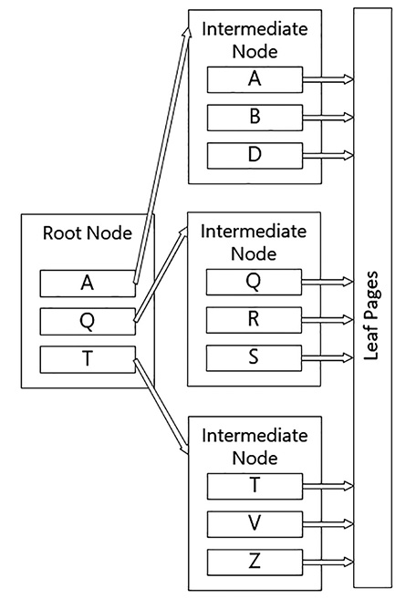
In the index shown in Figure 1-1, when you search for an item, if it is between A and Q, you follow the pointer to the first intermediate node of the tree. This structure is repeated for as many levels as there are in the index. When you reach the last intermediate node (which may be the root node for smaller indexes), you go to the leaf node.

There are two types of indexes in SQL Server: clustered and non-clustered. Clustered indexes are indexes where the leaf node in the tree contains the actual data in the table (A table without a clustered index is a heap which is made up of non-sequential, 8K pages of data.) A non-clustered index is a separate structure that has a copy of data in the leaf node that is in the keys, along with a pointer to the heap or clustered index.

The structure of the non-clustered leaf pages depends on whether the table is a heap or a clustered table. For a heap, it contains a pointer to the physical structure where the data resides. For a clustered table, it contains the value of the clustered index keys (referred to as the clustering key.) Last, for a clustered columnstore index, it is the position in the columnstore index (covered in Skill 1.4).

When the index key is a single column, it is referred to as a simple index, and when there are multiple columns, it is called a composite index. The index nodes (and leaf pages) will be sorted in the order of the leading column first, then the second column, etc. For a composite index it is best to choose the column that is the most selective for the lead column, which is to say, it has the most unique values amongst the rows of the table.

The limit on the size of index key (for the data in all of the columns declared for the index) is based on the type of the index. The maximum key size for a non-clustered index is 1700 bytes, and 900 for a clustered index. Note that the smaller the index key size, the more that fits on each index level, and the fewer index levels, the fewer reads per operation. A page contains a maximum of 8060 bytes, and there is some overhead when storing variable length column values. If your index key values are 1700 bytes, which means you could only have 4 rows per page. In a million row table, you can imagine this would become quite a large index structure.

During the database design phase

During the coding phase, continuing throughout the lifecycle of your implementation

The primary difference between the two phases is need. During the design phase, there are constraints that create indexes as part of their creation, and a few situations where it is essential to create an index without even executing a query. After you have configured your tables, the goal of indexes is almost completely aligned to how well your queries work, and you must add indexes where the need arises, and not just because it seems like a good idea.

Uniqueness Constraints PRIMARY KEY and UNIQUE constraints automatically create an index.

Foreign Key Columns Columns that reference a FOREIGN KEY constraint are often, but not always a likely target for an index.

Let’s explore these two situations.

As an example, consider the following table structure:

Click here to view code image

CREATE TABLE Examples.UniquenessConstraint
(
    PrimaryUniqueValue int NOT NULL,
    AlternateUniqueValue1 int NULL,
    AlternateUniqueValue2 int NULL
);

When you have a value that you need to be the primary key value, you can use a PRIMARY KEY constraint. So, using ALTER TABLE (or inline as part of the initial CREATE TABLE statement) you can add:

Click here to view code image

ALTER TABLE Examples.UniquenessConstraint
    ADD CONSTRAINT PKUniquenessContraint PRIMARY KEY (PrimaryUniqueValue);

A PRIMARY KEY constraint cannot be placed on a column that allows NULL values, and you get an error if you try (or in a CREATE TABLE statement it sets the column to not allow NULL values). In cases where you have alternate columns that are used to identify a row (typical when you use an artificial surrogate value like a meaningless integer for a primary key, which is covered in Chapter 2 in more detail, you can add a UNIQUE constraint that can be placed on columns that allow NULL values, something demonstrated later in this section):

Click here to view code image

ALTER TABLE Examples.UniquenessConstraint
    ADD CONSTRAINT AKUniquenessContraint UNIQUE
          (AlternateUniqueValue1, AlternateUniqueValue2);

The uniqueness constraints created indexes with the same name as the constraints behind the scenes, which you can see in sys.indexes:

Click here to view code image

SELECT type_desc, is_primary_key, is_unique, is_unique_constraint
FROM   sys.indexes
WHERE  OBJECT_ID('Examples.UniquenessConstraint') = object_id;

This shows you that the index is clustered, and is unique.

Click here to view code image

name                 type_desc       is_primary_key is_unique is_unique_constraint
--------------------- --------------- -------------- --------- -------------------
PKUniquenessContraint CLUSTERED       1              1         0
AKUniquenessContraint NONCLUSTERED    0              1         1

When you have constraints on all of the data that needs to be unique for an OLTP database, you often have a large percentage of the indexes you need. OLTP databases are generally characterized by short transactions and simple queries, usually looking for one row (even if the query sometimes looks for a range of data because the user doesn’t know how to spell a given value.)

In Chapter 4, Skill 4.1, we discuss optimizing indexes, including how to determine if indexes are being used. However, indexes that are created by uniqueness constraints should not be considered for removal. Even if the index is never used to improve the performance of a query, it is essential to your data integrity to make sure that if a value is supposed to be unique, that a constraint ensures that values are unique. NULL values behave differently in UNIQUE indexes than in almost any other place in SQL Server. A PRIMARY KEY constraint does not allow any NULL values in columns, but a UNIQUE constraint and a unique index does. So, using the table we created, if we try creating the following rows:

Click here to view code image

INSERT INTO Examples.UniquenessConstraint
            (PrimaryUniqueValue, AlternateUniqueValue1, AlternateUniqueValue2)
VALUES (1, NULL, NULL), (2, NULL, NULL);

We then receive the following error message:

Click here to view code image

Msg 2627, Level 14, State 1, Line 95
Violation of UNIQUE KEY constraint 'AKUniquenessContraint'. Cannot insert duplicate key
in object 'Examples.UniquenessConstraint'. The duplicate key value is (<NULL>, <NULL>)

What is initially confusing about this is that we said earlier that NULL never was equal to NULL. This is still true, but in the index keys, two NULL values are treated as duplicate missing values.

Click here to view code image

--Represents an order a person makes, there are 10,000,000 + rows in this table
CREATE TABLE Examples.Invoice
(
    InvoiceId   int NOT NULL CONSTRAINT PKInvoice PRIMARY KEY,
    --Other Columns Omitted
);
--Represents a type of discount the office gives a customer,
--there are 200 rows in this table
CREATE TABLE Examples.DiscountType
(
    DiscountTypeId   int NOT NULL CONSTRAINT PKDiscountType PRIMARY KEY,
    --Other Columns Omitted
)
--Represents the individual items that a customer has ordered, There is an average of
--3 items ordered per invoice, so there are over 30,000,000 rows in this table
CREATE TABLE Examples.InvoiceLineItem
(
   InvoiceLineItemId int NOT NULL CONSTRAINT PKInvoiceLineItem PRIMARY KEY,
   InvoiceId int NOT NULL
          CONSTRAINT FKInvoiceLineItem$Ref$Invoice
                REFERENCES Examples.Invoice (InvoiceId),
   DiscountTypeId int NOT NULL
          CONSTRAINT FKInvoiceLineItem$Ref$DiscountType
                REFERENCES Examples.DiscountType (DiscountTypeId)
    --Other Columns Omitted
);

There are two foreign key columns in the InvoiceLineItem table to cover. The InvoiceId column has mostly unique values, with an average of 3 rows per invoice. It is also a typical thing a user might do; grabbing all of the invoice items for an invoice. Hence, that is a column that almost certainly benefits from an index (and as we discuss later in the section “Implement clustered index columns by using best practices”, perhaps even a clustered index if the reference is used frequently enough.) Create that index as a non-clustered index for now as:

Click here to view code image

CREATE INDEX InvoiceId ON Examples.InvoiceLineItem (InvoiceId);

When creating an index on a not-very selective column, like perhaps the DiscountTypeId, where out of 30 million rows, there are just 20 distinct values in 100000 rows. This column could benefit from a filtered index, which is an index that has a WHERE clause. So if almost all rows were NULL, it could be that searching for a row with the value of NULL in the index would be useless. However, a search for other values actually could use the index. So you could create a filtered index as:

Click here to view code image

CREATE INDEX DiscountTypeId ON Examples.InvoiceLineItem(DiscountTypeId)
                                           WHERE DiscountTypeId IS NOT NULL;

Filtered indexes can have any columns in the WHERE clause, even if not represented in the index keys or included columns (which we use later in this chapter in the section: “Distinguish between indexed columns and included columns”).

When creating an INDEX, if the data in the key columns is always unique (such as if the columns of the index are a superset of a UNIQUE and/or PRIMARY KEY constraint columns,) declare the index as UNIQUE, as in:

Click here to view code image

CREATE UNIQUE INDEX InvoiceColumns ON Examples.InvoiceLineItem(InvoiceId,
                                                               InvoiceLineItemId);

It is typically desirable to have indexes that enforce uniqueness to be based on a constraint, but this is not a requirement. Any UNIQUE index, even a filtered one, can be declared as only allowing unique values which will disallow duplicated index key values.

In the WideWorldImporters database, there are indexes on all of the foreign keys that were generated when creating that database. Beyond guessing what one can do to decide whether an index would be useful, it is essential to understand a query plan. Most of the figures in this chapter are query plans to demonstrate what is going on in the query optimizer and query processor. As an example, use one of the relationships in the WideWorldImporters database, between the Sales.CustomerTransactions and Application.PaymentMethods tables.

In the Sales.CustomerTransactions table, there are 97147 rows. The index on the foreign key column is non-clustered, so every use of the non-clustered index requires a probe of the clustered index to fetch the data (referred to as a bookmark lookup), so it is very unlikely the index is used for a predicate. Take a look at the data in the PaymentMethodId column:

Click here to view code image

SELECT PaymentMethodId, COUNT(*) AS NumRows
FROM   Sales.CustomerTransactions
GROUP  BY PaymentMethodID;

You can see that there are just two values in use:

Click here to view code image

PaymentMethodId NumRows
--------------- -----------
4               26637
NULL            70510

Take a look at the plan of the following query that the system might perform, searching for CustomerTransactions rows where the PaymentMethodId = 4:

Click here to view code image

SELECT *
FROM   Sales.CustomerTransactions
WHERE PaymentMethodID = 4;

This returns the expected 26637 rows, and has the actual plan shown in Figure 1-2. The Compute Scalar operator is there because we returned all columns, and there is a computed column in the table named IsFinalized.

There are three ways using the GUI to get the query plan. From the Query Menu, select:

1. Display Estimated Plan This shows you the plan that is likely to be used to perform the query. The plan can change when the query is performed, due to many factors such as query load, memory available, etc. All row counts and costs are guesses based on the statistics of the index, and it does not require the query to be performed. Whether or not parallelism can be used is determined during execution based on system settings (such as the sp_configure setting ‘cost threshold for parallelism’ and ‘max degree of parallelism’) and the load on the system at execution time.

2. Include Actual Execution Plan This represents the plan that is used, including actual row counts, use of parallelism, etc. You get the actual plan after the query has completed in its entirety.

3. Include Live Query Statistics When you are working with a complex, long-running query, you can see data moving through the actual query plan operators live. It can help you diagnose issues with a large query by letting you see the problem spots in real time.

For now, we ignore the Missing Index listed in the plan (and for future cases edit them out until we get to the section on “Included Columns”), but the point here is that the index was not used. However, it is important to note that while an index is not generally useful, there are scenarios where the index actually turns out to be useful:

If the only column that was returned from the query was the PaymentMethodId since all of the data is there in the index, then it is useful.

An index is also useful when you are searching for a value that does not exist in the table. The statistics of the index do not tell the optimizer that no rows are returned from the query, only that very few are returned, so using the index should be fast enough. We review managing statistics in more detail in Chapter 4, but they are basically structures that help the optimizer to guess how many rows are returned by a given query based on a sampling of the data at a given point in time.

These scenarios are why foreign key indexes are often applied to all foreign key columns, even if the indexes applied are not generally useful.

Common search paths

Joins

Sorting data

Unless you have very simplistic needs, it is hard to know exactly how queries behave in a real scenario, so in most cases it is better to test out your expectations rather than guess about performance.

Click here to view code image

SELECT CustomerID, OrderID, OrderDate, ExpectedDeliveryDate
FROM Sales.Orders
WHERE CustomerPurchaseOrderNumber = '16374';

The query runs quickly in the default set of rows in the Sales.Orders table, returning only 6 rows. The amount of time the query takes, using the small-sized dataset, seems adequate. However, to dig deeper and find out how well the query actually performs, you can use two commands in Transact-SQL to see some very important statistics. The statistics, along with the query plan will give you deeper insight into how the query is operating.

Click here to view code image

SET STATISTICS TIME ON;
SET STATISTICS IO ON;

SELECT CustomerID, OrderId, OrderDate, ExpectedDeliveryDate
FROM  Sales.Orders
WHERE CustomerPurchaseOrderNumber = '16374';

SET STATISTICS TIME OFF;
SET STATISTICS IO OFF;

The plan returns what is shown in Figure 1-3.

Along with the query results, there are a few additional messages. We are reducing to the pertinent ones here in our output, but you can see the compile and parse times, and the overall execution time in addition to the following:

Click here to view code image

Table 'Orders'. Scan count 1, logical reads 692, physical reads 0, read-ahead reads 0,
lob logical reads 0, lob physical reads 0, lob read-ahead reads 0.

 SQL Server Execution Times:
   CPU time = 15 ms,  elapsed time = 20 ms.:

The query only takes around 20 milliseconds (ms) on my VM (Surface Pro 4 with 16 GB of RAM, and 8GB for the VM), scanning the entire table, and touching all 692 pages containing 73595 rows. The pages are all in RAM, so there are no physical reads. This is very common when testing individual queries, so there is no memory pressure. (You can clear the cache using DBCC DROPCLEANBUFFERS, but the most important number for indexing is logical reads. Consistent readings of a large number of physical reads are more indicative of not enough RAM to cache data). However, if this is a table to which data is being actively written, scanning those 692 pages means that every single row is touched, and therefore locked for some amount of time, causing concurrency issues that are covered in more detail in Chapter 3, “Manage Database Concurrency.”

Next, add an index to the Sales.Orders table on just the CustomerPurchaseOrderNumber column, in attempt to make the query perform better.

Click here to view code image

CREATE INDEX CustomerPurchaseOrderNumber ON Sales.Orders(CustomerPurchaseOrderNumber);

Now, perform the same query on CustomerPurchaseOrderNumber = ‘16374’, and the following query plan is used, as shown in Figure 1-4.

The query plan looks more complex. There is a join, even though the query uses a single table. SQL Server now uses the index-seek operation to find the six matching rows, but all it has are the CustomerID and the OrderID from the index keys. So it needs to use a JOIN operator to join to the clustered index to get the rest of the data. While the plan is more complex, the results are a lot better statistically, as you can see:

Click here to view code image

Table 'Orders'. Scan count 1, logical reads 20, physical reads 0, read-ahead reads 0,
lob logical reads 0, lob physical reads 0, lob read-ahead reads 0.
 SQL Server Execution Times:
   CPU time = 0 ms,  elapsed time = 0 ms.

It took only 20 logical reads, and less than 1 millisecond to perform. The reduction in 672 reads, means 672 less physical resources touched, and locked by default. As a result, it is very useful to check out all of the queries that are used by your applications, either (ideally) from stored procedures, or as ad-hoc queries performed from your external interfaces.

Note that you can index a computed column as long as it is deterministic. You can tell if a column can be indexed, even if it is computed by using the COLUMNPROPERTYEX() function:

Click here to view code image

SELECT CONCAT(OBJECT_SCHEMA_NAME(object_id), '.', OBJECT_NAME(object_id)) AS TableName,
       name AS ColumnName, COLUMNPROPERTYEX(object_id, name, 'IsIndexable') AS Indexable
FROM   sys.columns
WHERE is_computed = 1;

Search conditions are typically the most obvious to index because they affect people directly. When a user searches on an unindexed column in a large table (relative to hardware capabilities), you may see locking, blocking, or using some settings (such as the database setting READ COMMITTED SNAPSHOT), high tempdb utilization. The needs are more random than in the following situation we will cover.

As an example, drop the foreign key index from the Sales.Orders table named FK_Sales_Orders_ContactPersonID using the following command:

Click here to view code image

DROP INDEX FK_Sales_Orders_ContactPersonID ON Sales.Orders;

Now, search for the Sales.Orders rows for any person with a preferred name of ‘Aakriti:’

Click here to view code image

SELECT OrderId, OrderDate, ExpectedDeliveryDate, People.FullName
FROM  Sales.Orders
        JOIN Application.People
            ON People.PersonID = Orders.ContactPersonID
WHERE  People.PreferredName = 'Aakriti';

The PreferredName column is not indexed. Figure 1-5 shows the actual query plan, along with the typical query stats output.

Figure 1-5 has the following output:

Click here to view code image

Table 'Workfile'. Scan count 0, logical reads 0, physical reads 0, read-ahead reads 0,
lob logical reads 0, lob physical reads 0, lob read-ahead reads 0.

Table 'Worktable'. Scan count 0, logical reads 0, physical reads 0, read-ahead reads 0,
lob logical reads 0, lob physical reads 0,

lob read-ahead reads 0.

Table 'Orders'. Scan count 1, logical reads 692, physical reads 0, read-ahead reads 0,
lob logical reads 0, lob physical reads 0,

lob read-ahead reads 0.

Table 'People'. Scan count 1, logical reads 80, physical reads 0, read-ahead reads 0,
lob logical reads 0, lob physical reads 0,

lob read-ahead reads 0.

CPU time = 15 ms,  elapsed time = 53 ms.

Hovering your mouse over the Clustered Index Scan operator for the PK_Application_People index (the clustered index on the table), you see (as depicted in Figure 1-6) the costs, but also that the predicate of PreferredName = ‘Aakriti’ is handled as part of this scan.

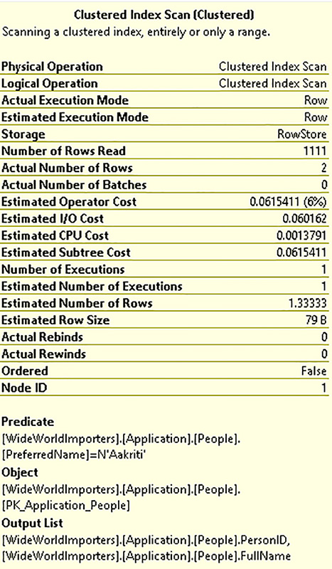
As you can see, the query optimizer scans the two indexes, and the Hash Match operator builds a hash index structure, and then matches the rows together. Adding back the index on the foreign key columns:

Click here to view code image

CREATE INDEX FK_Sales_Orders_ContactPersonID ON Sales.Orders
--Note that USERDATA is a filegroup where the index was originally
              (ContactPersonID ASC ) ON USERDATA;

Executing the query again shows a better result, though not tremendously, as shown in Figure 1-7.

Figure 1-7 has the following output:

Click here to view code image

Table 'Orders'. Scan count 2, logical reads 695, physical reads 0, read-ahead reads 0,
lob logical reads 0, lob physical reads 0,

lob read-ahead reads 0.

Table 'People'. Scan count 1, logical reads 80, physical reads 0, read-ahead reads 0,
lob logical reads 0, lob physical reads 0,

lob read-ahead reads 0.

CPU time = 0 ms,  elapsed time = 17 ms.

The big cost here is the Key Lookup operator to fetch the rest of the Sales.Orders columns in our query. This cost is what the missing index hint has been suggesting for nearly every query, and is the topic of the next section of this chapter. The query can be improved upon one more time by indexing the PreferredName column, so the query processor doesn’t have to test every single row in the Application.People table to see if it matches PreferredName = ‘Aakriti’.

Click here to view code image

CREATE INDEX PreferredName ON Application.People (PreferredName) ON USERDATA;

Finally, perform the query again to see the plan and statistics shown in Figure 1-8.

Figure 1-8 has the following output:

Click here to view code image

Table 'Orders'. Scan count 2, logical reads 695, physical reads 0, read-ahead reads 0,
lob logical reads 0, lob physical reads 0,

lob read-ahead reads 0.

Table 'People'. Scan count 1, logical reads 6, physical reads 0, read-ahead reads 0, lob
logical reads 0, lob physical reads 0, lob read-ahead reads 0.

CPU time = 0 ms,  elapsed time = 19 ms.

This is not a tremendous improvement, and is just 74 less accessed pages, and execution times are typically the same. Generally speaking though, the fewer pages read in the process of executing the query, the better, particularly as the number of queries increase in an active system.

Note the Key Lookup operator that is 97 percent of the cost of this query. In a following section on included columns, we review how to erase that cost, and lower the logical reads to very few.

A part of the CREATE INDEX statement we have not yet looked at is sorting of the index keys, particularly useful with composite index keys. By default, the data in the index is sorted in ascending order, so the indexes created so far have been ascending by default. The query processor can scan the index in either direction, so for a simple index (one with a single key column), this is generally not a problem. For composite indexes (those with greater than a single key column) it can be an issue.

As an example, consider the following query of the entire Sales.Orders table, sorted in SalespersonPersonID and OrderDate order. Both are explicitly spelled out as ASC, meaning ascending, which is the default. Note too that we only return the columns that are being sorted on to make the example simpler.

Click here to view code image

SELECT SalespersonPersonId, OrderDate
FROM Sales.Orders
ORDER BY SalespersonPersonId ASC, OrderDate ASC;

Figure 1-9 shows the plan, which includes a scan through the data, a sort, and it even shows that the query used parallelism, since we’re running on a VM with 2 CPUs allocated. In other words, this was not a trivial query.

Figure 1-9 has the following output:

Click here to view code image

Table 'Worktable'. Scan count 0, logical reads 0, physical reads 0, read-ahead reads 0,
lob logical reads 0, lob physical reads 0,

lob read-ahead reads 0.

Table 'Orders'. Scan count 3, logical reads 758, physical reads 0, read-ahead reads 0,
lob logical reads 0, lob physical reads 0,

lob read-ahead reads 0.

CPU time = 94 ms,  elapsed time = 367 ms.

Now, add an index to support this query, as we know that this query is performed very often in our enterprise. Add a composite index, and explicitly show that we are sorting the keys in ascending order, for the query:

Click here to view code image

CREATE INDEX SalespersonPersonID_OrderDate ON Sales.Orders
                              (SalespersonPersonID ASC, OrderDate ASC);

Perform the query just as we did in the first attempt. Figure 1-10, shows that the plan has changed, as now it can get the data in a pre-sorted manner, with the primary cost of the query now embedded in the bookmark lookup.

Figure 1-10 has the following output:

Click here to view code image

Table 'Orders'. Scan count 1, logical reads 157, physical reads 0, read-ahead reads 0,
lob logical reads 0, lob physical reads 0, lob read-ahead reads 0.

CPU time = 47 ms,  elapsed time = 217 ms.

If the order you request is completely opposite of how the index is sorted, you will find that nothing in the plan will change:

Click here to view code image

SELECT SalespersonPersonId, OrderDate
FROM Sales.Orders
ORDER BY SalespersonPersonId DESC, OrderDate DESC;

If your sorting needs don’t match the index exactly, it’s still useful to the query, but only until there is a mismatch. For example, change the ORDER BY to either of the following (DESC is descending):

ORDER BY SalespersonPersonId DESC, OrderDate ASC;

ORDER BY SalespersonPersonId ASC, OrderDate DESC;

And you see the plan changes to what is shown in Figure 1-11.

The query processor was able to skip sorting the data based on the first column by using the index, but then it had to sort the second column using a separate operator, rather than just scanning the data in order. As such, it is important to note the order of the columns in the ORDER BY clause, if you were given a question matching the index with the ORDER BY clause.

One place where sorting often is helped by indexes is when joining two large sets. The query plan can use a Merge Join operator to join two sorted sets together, by matching item after item, since they are in sorted order. As an example, take a join of two tables, the Sales.Orders and the Application.People, returning all of the rows in the tables, but just their key values:

Click here to view code image

SELECT Orders.ContactPersonID, People.PersonID
FROM   Sales.Orders
         INNER JOIN Application.People
            ON Orders.ContactPersonID = People.PersonID;

Executing this, you see that since there is an index on the foreign key column in Sales.Orders, and the PRIMARY KEY constraint on the Application.People table, the data is sorted, so it can use a Merge Join operator, as seen in Figure 1-12.

To be entirely fair, the output of this query is nonsensical because it returns two columns that are equivalent in all 72,595 rows. However, when you are doing joins between multiple tables, you often see a Merge Join operator appear in plans when nothing but indexed columns are accessed from the tables that are being joined.

Carefully consider how you use non-clustered indexes to support sorts, as the cost of the bookmark lookup often tips the plan towards using a scan of the base structure.

However, as the number of rows you return grows, the bookmark lookup operations become more and more of a drag on performance. When you need to run a query that returns a lot of rows, but doesn’t need all of the data in the table, there is a feature known as included columns that allows you to use an index to cover the entire needs of the query. When an index has all of the data that is needed to return the results of a query, either in the key columns, or included columns, it is referred to as a covering index for a query.

As an example, take a look back at this query we have used previously:

Click here to view code image

SELECT OrderId, OrderDate, ExpectedDeliveryDate, People.FullName
FROM  Sales.Orders
        JOIN Application.People
            ON People.PersonID = Orders.ContactPersonID
WHERE  People.PreferredName = 'Aakriti';

Remember back in Figure 1-11, this query was very efficient in terms of finding the rows that needed to be returned in the Sales.Orders table, but had one operator that was 97 percent of the cost of execution, and required 695 pages to be read in the Sales.Orders table.

Now perform the query, and see the plan that is output. In the plan shown in Figure 1-13, the Key Lookup operator is 97% of the overall cost of the query. There are two Key Lookup operators in the plan, so remove both of them in the simplest case.

Figure 1-13 has the following output:

Click here to view code image

Table 'Orders'. Scan count 2, logical reads 695, physical reads 0, read-ahead reads 0,
lob logical reads 0, lob physical reads 0,

lob read-ahead reads 0.

Table 'People'. Scan count 1, logical reads 6, physical reads 0, read-ahead reads 0, lob
logical reads 0, lob physical reads 0,

lob read-ahead reads 0.

CPU time = 0 ms,  elapsed time = 141 ms.

As a first step, if we simplify our query to just use the columns that are indexed, the Sales.Orders.ContactPersonID column from the foreign key index that was created by the database designer, and the Application.People.PreferredName column (which also includes the PersonId since it is the clustering key), you see that all of the data you need for your query (for all clauses, SELECT, FROM, WHERE, etc) can be found in the index keys. Executing the query:

Click here to view code image

SELECT Orders.ContactPersonId, People.PreferredName
FROM  Sales.Orders
        JOIN Application.People
            ON People.PersonID = Orders.ContactPersonID
WHERE  People.PreferredName = 'Aakriti';

Now the query plan looks wonderful, and the number of logical reads are down dramatically, as you can see in Figure 1-14. The indexes that are being sought are covering the query processor’s needs. There is only one small problem. The query results are not even vaguely what the customer needs.

Figure 1-14 has the following output:

Click here to view code image

Table 'Orders'. Scan count 2, logical reads 4, physical reads 0, read-ahead reads 0, lob
logical reads 0, lob physical reads 0,

lob read-ahead reads 0.

Table 'People'. Scan count 1, logical reads 2, physical reads 0, read-ahead reads 0, lob
logical reads 0, lob physical reads 0,

lob read-ahead reads 0.

CPU time = 0 ms,  elapsed time = 38 ms.

In order to keep this performance with the minimum overhead, but providing results that were requested, you can use what is referred to as a covering index. The leaf nodes of a non-clustered index contains the value being indexed, along with a row locator. A covering index uses the INCLUDE keyword on the CREATE INDEX statement to include additional information on the leaf nodes. You can include any data type (even the large types like nvarchar(max), though the larger the data type, the less fits on a page, or it could even overflow to multiple pages.

For our two queries, we add another index to the Sales.Orders table (since the foreign key index came as part of the base installation) and replace the PreferredName index that is part of the original WideWorldImporters database.

Click here to view code image

CREATE NONCLUSTERED INDEX ContactPersonID_Include_OrderDate_ExpectedDeliveryDate
ON Sales.Orders ( ContactPersonID )
INCLUDE ( OrderDate,ExpectedDeliveryDate)
ON USERDATA;
GO

And to the PreferredName index we include the column the customer wanted, the FullName column.

Click here to view code image

DROP INDEX PreferredName ON Application.People;
GO
CREATE NONCLUSTERED INDEX PreferredName_Include_FullName
ON Application.People (      PreferredName )
INCLUDE (FullName)
ON USERDATA;

Now, perform the query:

Click here to view code image

SELECT OrderId, OrderDate, ExpectedDeliveryDate, People.FullName
FROM  Sales.Orders
        JOIN Application.People
            ON People.PersonID = Orders.ContactPersonID
WHERE  People.PreferredName = 'Aakriti';

And the plan now looks great, and returns what the customer needs. You can see the plan in Figure 1-15.

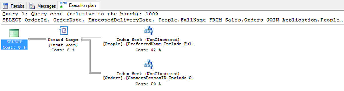
Figire 1-15 has the following output:

Click here to view code image

Table 'Orders'. Scan count 2, logical reads 6, physical reads 0, read-ahead reads 0, lob
logical reads 0, lob physical reads 0,

lob read-ahead reads 0.

Table 'People'. Scan count 1, logical reads 2, physical reads 0, read-ahead reads 0, lob
logical reads 0, lob physical reads 0,

lob read-ahead reads 0.

CPU time = 0 ms,  elapsed time = 79 ms.

Covering indexes are fantastic tools for tuning queries where you are dealing with costly Key Lookup operators. However, restraint should be taken when considering whether or not to apply them. When checking the plan of a query, you are frequently given a missing index hint that encourages you to add an index with a long list of included columns. Figure 1-5 showed the plan of the following query:

SELECT *

Click here to view code image

FROM   Sales.CustomerTransactions
WHERE PaymentMethodID = 4;

When looking at the plan, there was a missing index hint as shown in Figure 1-16.

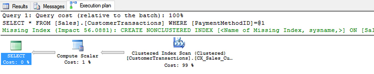
Hovering your cursor over the missing index shows you details in a tool-tip, or right click the plan and choose “Missing Index Details...” and you see the following index:

Click here to view code image

CREATE NONCLUSTERED INDEX [<Name of Missing Index, sysname,>]
ON [Sales].[CustomerTransactions] ([PaymentMethodID])
INCLUDE ([CustomerTransactionID],[CustomerID],[TransactionTypeID], [InvoiceID],[Transact
ionDate],[AmountExcludingTax],[TaxAmount],[TransactionAmount],
[OutstandingBalance],[FinalizationDate],[IsFinalized],[LastEditedBy],[LastEditedWhen])

Adding this index definitely increases the performance of your query. It reduces logical reads from 1126 to 312. This is not a tremendous savings, and likely doesn’t merit adding in a strict OLTP system, as for every change to the Sales.CustomerTransactions table, all of these column values are copied again to the index pages. For a reporting database, missing indexes can be great things to add, but you always need to take caution.

The Missing Indexes tip is basically where the optimizer was working through what it was looking for to perform the query the fastest, and an index that would have helped was discovered. In Chapter 4, “Optimize database objects and SQL infrastructure,” we explore the missing indexes dynamic management view (DMV) where you can see indexes that SQL Server would like to have had for the queries that have been optimized over time. Many of them overlap with other indexes that it has suggested. If you added all of the indexes that it suggested to a busy system, it would be brought to its knees maintaining indexes.

One last property of included columns is important to understand. Included columns in an index can never be used to seek for rows or for ordered scans (since they are not ordered at all), but they can be used to cover a query even if the key columns are not involved. For example, consider the following query that uses the columns that we indexed in the index named ContactPersonID_Include_OrderDate_ExpectedDeliveryDate. If we only reference the OrderDate and ExpectedDeliveryDate in a query, even as a predicate, the index can be scanned instead of the (typically) much larger data in the base table. Take the following query:

Click here to view code image

SELECT OrderDate, ExpectedDeliveryDate
FROM  Sales.Orders
WHERE OrderDate > '2015-01-01';

Figure 1-17 shows that it uses the index with included columns:

Of course, this is not the optimum index for the query, so the query plan suggests the following index, which orders the data on the OrderDate, and includes the ExpectedDeliveryDate as an included column:

Click here to view code image

CREATE NONCLUSTERED INDEX [<Name of Missing Index, sysname,>]
ON [Sales].[Orders] ([OrderDate])
INCLUDE ([ExpectedDeliveryDate]);

Take caution when using the missing index hints (or missing indexes DMV that are reviewed in Chapter 4.) They are not the best for your system’s overall performance, which certainly could be a topic on the exam. Still, covering queries using the INCLUDE feature is a great way to improve situations where a read-intensive workload is using scans to resolve queries because of a few columns that could be added to the index leaf nodes.

The clustered index contains all of the data of the table on the leaf index pages (or at least the base structures, as data can overflow onto multiple pages for very large rows), so when the clustered index optimally satisfies the query’s needs, the performance of the query is going to be better than otherwise.

The clustering key (the term used for the key column(s) of the clustered index) affects the other row store indexes in the table. Picking a larger clustering key could be terrible for performance of all of the other indexes since every non-clustered index key carries this value around.

If the clustered index is not created as unique, when a duplicate key value is created, it has a four-byte uniqueifier attached to duplicated values to make it unique so it makes a proper row locator.

If you change the value of the clustering key, you change the data on every non-clustered rowstore index.

The best clustering key is an increasing value, as it is inserted at the end of the structure that is sorted, leading to minimized page splits. When a new row is created in the middle of the clustering key sequence, a large row causes the page split.

There is also a clustered columnstore index that we cover in Skill 1.4.

So with all of these limitations, what should you choose for the clustered index? There are a few key scenarios to look for:

The column(s) that are used for single row fetches, often for modifications Many OLTP databases operate by fetching a set of rows to a client, and then updating the rows, one at a time. Watching the patterns of usage can help, but almost all of the time the primary key fits this usage, whether the database is using a natural key as primary key, or an artificial surrogate key. An IDENTITY or SEQUENCE based artificial key meets all of the points we started out with, so when implementing a system with artificial keys, it is often the best choice.

Range queries Having all the data in a particular order can be essential to performance when the data that you often need to get a range. Even a range of 1 distinct value makes sense, for a situation like a child row, such as Invoice and InvoiceLineItem where you are constantly fetching InvoiceLineItem rows by the InvoiceId for the invoice.

Queries that return large result sets If you have a situation where a particular query (or set of queries) is run frequently and returns a lot of rows, performing these searches by clustered index can be beneficial.

The typical default that most designers use is to use the clustered index on columns of the primary key. It is always unique, and is almost certainly where the largest percentage of rows are fetched or the PRIMARY KEY constraint is likely misused. In a real database, this requires testing to see how it affects overall performance.

Instinctively, it seems that you want to use the value that the user does most searches on, but the reason that the index that backs the PRIMARY KEY constraint is chosen is because beyond searches, you see lots of fetches by the primary key since singleton SELECTs, UPDATEs, and DELETEs all typically use the primary key for access. Add to that how JOIN operations are done using the primary key, and there needs to be a very compelling case to use something other than the primary key.

What data type you choose for the clustering key is a matter of opinion and tooling. For the exam, it is good to understand the different possibilities and some of the characteristics of each, particularly when creating an artificial value for a key. Two choices stand out as very common approaches:

Integer Data types

GUIDs

It isn’t impossible to use different approaches to these, but these are very common in almost any database. In the WideWorldImporters database, all of the primary keys are based on integers. Integers are generally the favored method because they are very small, and are easy to create in a monotonically increasing sequence using the IDENTITY property on a column, or using a SEQUENCE object applied using a DEFAULT constraint.

While integer-based data types generally fit the pattern of a great clustering key, there is another possibility that is very common. Using the uniqueidentifier data type, you can store a standard GUID (Globally Unique Identifier). A major advantage of these values are that they can be generated outside of the database server by any client, unlike an integer value, due to concurrency concerns. However, a major downside is indexing them. They have a 16-byte binary value with a 36-character representation (which can be needed if you have a client that can’t handle a GUID), and they are random in nature in terms of sorting. This leads to data being spread around the indexing structures, causing fragmentation, which can reduce the system’s ability to scan the data (though this is a bit less of a concern when you have fast SSD drives). You can generate GUID values in the database using NEWID(), or, if you almost never have new values coming from the client, you can use NEWSEQUENTIALID() to generate GUID values that are always increasing, making it a slightly better clustering key than a normal GUID. (However, NEWSEQUENTIALID() even can’t be trusted completely because the sequence of GUIDs is not guaranteed to be sequential with other GUIDs created after a reboot.)

In the end, the question of clustering key is very much centered on performance of your queries. Using a natural key can be difficult due to the size of many natural keys, but at the same time, a lot matters about how the application works, and how it turns out that data is used.

In the code shown in Listing 1-1, we make a copy of a couple of tables from the WideWorldImporters database, with limited indexes to serve as an example.

LISTING 1-1 Setting up a scenario for demonstrating query plans and indexes

Click here to view code image

---

--2074 Rows
SELECT *
INTO   Examples.PurchaseOrders
FROM   WideWorldImporters.Purchasing.PurchaseOrders;

ALTER  TABLE Examples.PurchaseOrders
    ADD CONSTRAINT PKPurchaseOrders PRIMARY KEY (PurchaseOrderId);

--8367 Rows
SELECT *
INTO   Examples.PurchaseOrderLines
FROM   WideWorldImporters.Purchasing.PurchaseOrderLines;

ALTER  TABLE Examples.PurchaseOrderLines
    ADD CONSTRAINT PKPurchaseOrderLines PRIMARY KEY (PurchaseOrderLineID);

ALTER TABLE Examples.PurchaseOrderLines
    ADD CONSTRAINT FKPurchaseOrderLines_Ref_Examples_PurchaseOrderLines
        FOREIGN KEY (PurchaseOrderId) REFERENCES
                                      Examples.PurchaseOrders(PurchaseOrderId);

---

Then we execute the following two queries:

Click here to view code image

SELECT *
FROM   Examples.PurchaseOrders
WHERE  PurchaseOrders.OrderDate BETWEEN '2016-03-10' AND '2016-03-14';

SELECT PurchaseOrderId, ExpectedDeliveryDate
FROM   Examples.PurchaseOrders
WHERE  EXISTS (SELECT *
                FROM  Examples.PurchaseOrderLines
                WHERE PurchaseOrderLines.PurchaseOrderId =
                                               PurchaseOrders.PurchaseOrderID)
  AND  PurchaseOrders.OrderDate BETWEEN '2016-03-10' AND '2016-03-14' ;

Executing these queries returns two sets of 5 rows each, and will probably take much less than a second on any computer as there are not very many rows in these tables at all. Since the query executes so quickly, the developer may get the idea that the query’s performance is optimum, even though there will be many users, and much more data in the production version. Using the Query; Display Estimated Query Plan menu in SQL Server Management Studio, we view the estimated plan in Figure 1-18 for this query, to help determine if the query is optimum.

Even though the first query would have appeared to be the costliest from looking at the results (or at least the equivalent amount of cost, it returned all of the data in the table, while the other just two small columns, all from the same rows), we can see that the first query was considerably less costly. Note how there are hidden costs, such as using user-defined functions that may not show up in a query plan.

For an exam question, you might be asked what you can tell about the indexes on the table from the plan given. We can tell that both queries are scanning the entire physical structures they reference due to the Clustered Index Scan operators. This certainly means that no index is available on the OrderDate column of the Examples.PurchaseOrders table that can help make this query execute faster. Knowing the row counts, there must be statistics on the OrderDate column that tells the optimizer how many rows will likely match the predicate because the line from PKPurchaseOrders is much smaller than that from PKPurchaseOrderLines. You can see the row counts by hovering over the lines, as shown in Figure 1-19, which is a composite from both lines. (Statistics, their meaning, and how they can be incorrect at times is covered in Skill 4.1).

Even though it was estimated that approximately 9 rows met the criteria, the optimizer still chose to scan the Examples.PurchaseOrderLines table and use a Hash Match join operator. This is an indication that there is no index on the PurchaseOrderLines.PurchaseOrderId column. Notice that the Hash Match operator is a Left Semi Join. A semi join means that data is returned from the left input, and not the right. This tells you that the Hash Match operator is most likely implementing a filter via a subquery, and not a JOIN in the FROM clause of the query.

Another question you might be asked is what index or indexes are useful to optimize a query based on the plan. From the evidence presented in our example, we can possibly add two indexes. One of them is simple:

Click here to view code image

CREATE INDEX PurchaseOrderId ON Examples.PurchaseOrderLines (PurchaseOrderId);

This index is definite since the only data that is used in the Examples.PurchaseOrderLines table is the PurchaseOrderId. What is more complex is whether the following index would be valuable on OrderDate in Examples.PurchaseOrders.:

Click here to view code image

CREATE INDEX OrderDate ON Examples.PurchaseOrders (OrderDate);

Because of the bookmark lookup factor, and the smaller table, this index is not used for this query, and even more importantly for taking the exam. Without executing the query we could not accurately predict this. However, a better index that will be useful on any size table will include the ExpectedDeliveryDate column along with the OrderDate:

Click here to view code image

CREATE INDEX OrderDate_Incl_ExpectedDeliveryDate
     ON Examples.PurchaseOrders (OrderDate) INCLUDE (ExpectedDeliveryDate);

This is because it covers all of the data needed to answer the conditions of the query. On the exam, it will be important to watch for conditions like this, where you are looking for the best answer that is always correct.

Reading a query plan is an essential developer skill, and should be expected on the exam since it is called out specifically in the indexes skill, and skill 4.2 is entitled “Analyze and troubleshoot query plans.” All throughout this chapter you will find query plans to demonstrate multiple scenarios you can see from the query plan. It is the primary way that we can tell how well a query is tuned.