The basic form of a view is very straightforward:

Click here to view code image

CREATE VIEW SchemaName.ViewName
[WITH OPTIONS]
AS SELECT statement
[WITH CHECK OPTION]

The SELECT statement can be as complex as you desire, and can use CTEs, set operators like UNION and EXCEPT, and any other constructs you can use in a single statement.

The options you can specify are:

SCHEMABINDING Protects the view from changes to the objects used in the SELECT statement. For example, if you reference Table1.Column1, the properties of that Column1 cannot be changed, nor can Table1 be dropped. Columns, not references can be removed, or new columns added.

VIEW_METADATA Alters how an application that accesses the VIEW sees the metadata. Typically, the metadata is based on the base tables, but VIEW_METADATA returns the definition from the VIEW object. This can be useful when trying to use a view like a table in an application.

ENCRYPTION Encrypts the entry in sys.syscomments that contains the text of the VIEW create statement. Has the side effect of preventing the view from being published as part of replication.

THE WITH CHECK OPTION will be covered in more detail later in this skill, but it basically limits what can be modified in the VIEW to what could be returned by the VIEW object.

For the most part, views are used for one specific need: to query simplification to encapsulate some query, or part of query, into a reusable structure. As long as they are not layered too deeply and complexly, this is a great usage. The following are a few specific scenarios to consider views for:

Hiding data for a particular purpose A view can be used to present a projection of the data in a table that limits the rows that can be seen with a WHERE clause, or by only returning certain columns from a table (or both).

Reformatting data In some cases, there is data in the source system that is used frequently, but doesn’t match the need as it stands. Instead of dealing with this situation in every usage, a view can provide an object that looks like the customer needs.

Reporting Often to encapsulate a complex query that needs to perform occasionally, and even some queries that aren’t exactly complicated, but they are performed repeatedly. This can be for use with a reporting tool, or simply for ad-hoc usage.

Providing a table-like interface for an application that can only use tables Sometimes a stored procedure makes more sense, but views are a lot more general purpose than are stored procedures. Almost any tool that can ingest and work with tables can use a view.

Let’s examine these scenarios for using a VIEW object, except the last one. That particular utilization is shown in the next section on updatable views. Of course, all of these scenarios can sometimes be implemented in the very same VIEW, as you might just want to see sales for the current year, with backordered and not shipped products grouped together for a report, and you might even want to be able to edit some of the data using that view. While this might be possible, we look at them as individual examples in the following sections.

A view might be created as shown in Listing 1-2.

LISTING 1-2 Creating a view that meets the user requirements

Click here to view code image

---

CREATE VIEW Sales.Orders12MonthsMultipleItems
AS
SELECT OrderId, CustomerID, SalespersonPersonID, OrderDate, ExpectedDeliveryDate
FROM   Sales.Orders
WHERE  OrderDate >= DATEADD(Month,-12,SYSDATETIME())
  AND (SELECT COUNT(*)
       FROM   Sales.OrderLines
       WHERE  OrderLines.OrderID = Orders.OrderID) > 1;

---

Now the user can simply query the data using this view, just like a table:

Click here to view code image

SELECT TOP 5 *
FROM   Sales.Orders12MonthsMultipleItems
ORDER BY ExpectedDeliveryDate desc;

Using TOP this returns 5 rows from the table:

Click here to view code image

OrderId     CustomerID  SalespersonPersonID OrderDate  ExpectedDeliveryDate
----------- ----------- ------------------- ---------- --------------------
73550       967         15                  2016-05-31 2016-06-01
73549       856         16                  2016-05-31 2016-06-01
73548       840         3                   2016-05-31 2016-06-01
73547       6           14                  2016-05-31 2016-06-01
73546       810         3                   2016-05-31 2016-06-01

Note that this particular usage of views is not limited to security like using row-level security might be. A user who has access to all of the rows in the table can still have a perfectly valid reason to see a specific type of data for a purpose.

Click here to view code image

SELECT PersonId, IsPermittedToLogon, IsEmployee, IsSalesPerson
FROM   Application.People;

What you see is 1111 rows of kind of cryptic data to look at (showing the first four rows):

Click here to view code image

PersonId    IsPermittedToLogon IsEmployee IsSalesPerson
----------- ------------------ ---------- -------------
1           0                  0          0
2           1                  1          1
3           1                  1          1
4           1                  1          0

A common request from a user that needs to look at this data using Transact-SQL could be: “I would like to see the data in the People table in a more user friendly manner. If the user can logon to the system, have a textual value that says ‘Can Logon’, or ‘Can’t Logon’ otherwise. I would like to see employees typed as ‘SalesPerson’ if they are, then as ‘Regular’ if they are an employee, or ‘Not Employee’ if they are not an employee.”

In Listing 1-3 is a VIEW object that meets these requirements.

LISTING 1-3 Creating the view reformat some columns in the Application.People table

Click here to view code image

---

CREATE VIEW Application.PeopleEmployeeStatus
AS
SELECT PersonId, FullName,
       IsPermittedToLogon, IsEmployee, IsSalesPerson,
       CASE WHEN IsPermittedToLogon = 1 THEN 'Can Logon'
             ELSE 'Can''t Logon' END AS LogonRights,
       CASE WHEN IsEmployee = 1 and IsSalesPerson = 1
                THEN 'Sales Person'
            WHEN IsEmployee = 1
                THEN 'Regular'
            ELSE 'Not Employee' END AS EmployeeType
FROM   Application.People;

---

Now, querying the data in the same manner (leaving off names), you see something more pleasant to work with:

Click here to view code image

SELECT PersonId, LogonRights, EmployeeType
FROM   Application.PeopleEmployeeStatus;

Which returns:

Click here to view code image

PersonId    LogonRights EmployeeType
----------- ----------- -------------
1           Can't Logon Not Employee
2           Can Logon   Sales Person
3           Can Logon   Sales Person
4           Can Logon   Regular

There is one serious downside to this method of reformatting. While this looks better, and is easier to see, queries that use the reformatted values to filter on the new columns never use an index since the data does not match what is in the index. For a smaller table, this isn’t an issue, but it is a concern. We included the columns in the view that had the original data for that reason.

A final concern is not to use views as layers of encapsulation in your application code for that same reason. The more layers of views you have, the less likely you get a great plan of execution. Views are definitely useful to have for morphing a set for many reasons, particularly when a user is repeatedly doing the same kinds of transformations in their code.

Requirements might be given to “Build a simple reporting interface that allows us to see sales profit or net income broken down by city, state, or territory customer category for the current week, up to the most current data”. If the system is normalized, there are quite a few tables involved in the query. Note that an important part of these requirements is that it be up to the most current data. If it did not include the most recent data, a data warehousing solution with a separate database would likely be more efficient.

In Listing 1-4, the code for the view that gives you a structure that can easily be used for providing these answers is included. The object is in a new schema named Reports to segregate it from other bits of code, and the view is suffixed “Basis” because this view could be the basis of several reports.

There are not any locking or isolation hints, and it is generally not a good practice to do so in your code unless using the SNAPSHOT isolation level in your database. Chapter 3 covers concurrency, isolation levels, in more detail.

LISTING 1-4 Creating the view that is the basis of an Invoice Summary report

Click here to view code image

---

CREATE SCHEMA Reports;
GO
CREATE VIEW Reports.InvoiceSummaryBasis
AS
SELECT Invoices.InvoiceId, CustomerCategories.CustomerCategoryName,
       Cities.CityName, StateProvinces.StateProvinceName,
       StateProvinces.SalesTerritory,
       Invoices.InvoiceDate,
       --the grain of the report is at the invoice, so total
       --the amounts for invoice
       SUM(InvoiceLines.LineProfit) as InvoiceProfit,
       SUM(InvoiceLines.ExtendedPrice) as InvoiceExtendedPrice
FROM   Sales.Invoices
         JOIN Sales.InvoiceLines
            ON Invoices.InvoiceID = InvoiceLines.InvoiceID
         JOIN Sales.Customers
              ON Customers.CustomerID = Invoices.CustomerID
         JOIN Sales.CustomerCategories
              ON Customers.CustomerCategoryID =
                               CustomerCategories.CustomerCategoryID
         JOIN Application.Cities
              ON Customers.DeliveryCityID = Cities.CityID
         JOIN Application.StateProvinces
              ON StateProvinces.StateProvinceID = Cities.StateProvinceID
GROUP BY Invoices.InvoiceId, CustomerCategories.CustomerCategoryName,
       Cities.CityName, StateProvinces.StateProvinceName,
       StateProvinces.SalesTerritory,
       Invoices.InvoiceDate;

---

Now you can create a report of the top 5 Sales by SalesTerritory pretty simply:

Click here to view code image

SELECT TOP 5 SalesTerritory, SUM(InvoiceProfit) AS InvoiceProfitTotal
FROM Reports.InvoiceSummaryBasis
WHERE InvoiceDate > '2016-05-01'
GROUP BY SalesTerritory
ORDER BY InvoiceProfitTotal DESC;

This returns:

Click here to view code image

SalesTerritory           InvoiceProfitTotal
------------------------ ---------------------
Southeast                536367.60
Great Lakes              366182.65
Mideast                  344703.00
Southwest                344386.95
Plains                   288766.20

Or, using the same structure, the top five sales by state and customer category:

Click here to view code image

SELECT TOP 5 StateProvinceName, CustomerCategoryName,
       SUM(InvoiceExtendedPrice) AS InvoiceExtendedPriceTotal
FROM Reports.InvoiceSummaryBasis
WHERE InvoiceDate > '2016-05-01'
GROUP BY StateProvinceName, CustomerCategoryName
ORDER BY InvoiceExtendedPriceTotal DESC;

This returns:

Click here to view code image

StateProvinceName    CustomerCategoryName   InvoiceExtendedPriceTotal
-------------------- ---------------------- ---------------------------------------
Texas                Novelty Shop           229966.31
Pennsylvania         Novelty Shop           210254.62
Ohio                 Novelty Shop           201242.59
New York             Novelty Shop           197664.32
California           Novelty Shop           178698.48

Clearly, novelty shops are a big business for WideWorldImporters. Looking at the plans of both queries, you should notice a couple of things. The plans are pretty large, not surprising since we joined a lot of tables. Nothing stands out as too terrible, and both plans suggest the same index:

Click here to view code image

CREATE NONCLUSTERED INDEX [<Name of Missing Index, sysname,>]
         ON [Sales].[Invoices] ([InvoiceDate]) INCLUDE ([InvoiceID],[CustomerID]);

There is no need to actually apply the index, but as we have discussed frequently, having a covering index for almost every query is a very common desire of the optimizer, and is not always a bad idea when you are doing ranges queries on the table (which was one of the strengths of the clustered index, because it had all of the data sorted for the range. Covering the data needs of queries make a non-clustered index with included columns behave like a clustered index for queries such as this.)

To provide interfaces with views there are some special configurations that you need to know. We look at the following scenarios for using views to modify tables.

Modifying views that reference one table

Limiting what data can be added to a table through a view through DDL

Modifying data in views with more than one table

LISTING 1-5 Creating the table and some data that is the basis of the updatable view example

Click here to view code image

---

CREATE TABLE Examples.Gadget
(
    GadgetId    int NOT NULL CONSTRAINT PKGadget PRIMARY KEY,
    GadgetNumber char(8) NOT NULL CONSTRAINT AKGadget UNIQUE,
    GadgetType  varchar(10) NOT NULL
);
INSERT INTO Examples.Gadget(GadgetId, GadgetNumber, GadgetType)
VALUES  (1,'00000001','Electronic'),
        (2,'00000002','Manual'),
        (3,'00000003','Manual');

---

When building a view to be editable, the simpler the view, the easier it is when you’re working with it. In the code that you see in Listing 1-6, there is a column that is the uppercase version of the gadget type to show how a non-executable column behaves.

LISTING 1-6 Creating the view that is the basis of an Invoice Summary report

Click here to view code image

---

CREATE VIEW Examples.ElectronicGadget
AS
    SELECT GadgetId, GadgetNumber, GadgetType,
           UPPER(GadgetType) AS UpperGadgedType
    FROM   Examples.Gadget
    WHERE GadgetType = 'Electronic';

---

Now, any user who is granted access to this view can only see rows that meet the WHERE clause of GadgetType = ‘Electronic’.

Next, perform the following query that shows you the data in the table, seeing what data the user sees:

Click here to view code image

SELECT ElectronicGadget.GadgetNumber AS FromView, Gadget.GadgetNumber AS FromTable,
        Gadget.GadgetType, ElectronicGadget.UpperGadgetType
FROM   Examples.ElectronicGadget
         FULL OUTER JOIN Examples.Gadget
            ON ElectronicGadget.GadgetId = Gadget.GadgetId;

You can see that for rows where the GadgetType <> ‘Electronic’:

Click here to view code image

FromView FromTable GadgetType UpperGadgetType
-------- --------- ---------- ---------------
00000001 00000001  Electronic ELECTRONIC
NULL     00000002  Manual     NULL
NULL     00000003  Manual     NULL

Now we run three statements to create some new rows, delete two rows, and update two rows in the table. In the comments on the code, include details of what you’re doing. First, try creating two new rows, referencing the derived column:

Click here to view code image

INSERT INTO Examples.ElectronicGadget(GadgetId, GadgetNumber,
                                      GadgetType, UpperGadgetType)
VALUES (4,'00000004','Electronic','XXXXXXXXXX'), --row we can see in view
       (5,'00000005','Manual','YYYYYYYYYY'); --row we cannot see in view

This fails, as you would expect:

Click here to view code image

Msg 4406, Level 16, State 1, Line 433
Update or insert of view or function 'Examples.ElectronicGadget' failed because
it contains a derived or constant field.

Now, try again, not referencing the calculated column:

Click here to view code image

INSERT INTO Examples.ElectronicGadget(GadgetId, GadgetNumber, GadgetType)
VALUES (4,'00000004','Electronic'),
       (5,'00000005','Manual');

This succeeds, so now use the query with the FULL OUTER JOIN from before, but limit it to the rows you created.

Click here to view code image

SELECT ElectronicGadget.GadgetNumber as FromView, Gadget.GadgetNumber as FromTable,
        Gadget.GadgetType, ElectronicGadget.UpperGadgetType
FROM   Examples.ElectronicGadget
         FULL OUTER JOIN Examples.Gadget
            ON ElectronicGadget.GadgetId = Gadget.GadgetId;

WHERE Gadget.GadgetId in (4,5);

Both rows were created, even though you cannot see the row in the view after the
operation:

FromView FromTable GadgetType UpperGadgetType
-------- --------- ---------- ---------------
00000004 00000004  Electronic ELECTRONIC
NULL     00000005  Manual     NULL

Next, update two rows:

Click here to view code image

--Update the row we could see to values that could not be seen
UPDATE Examples.ElectronicGadget
SET    GadgetType   = 'Manual'
WHERE  GadgetNumber = '00000004';

--Update the row we could see to values that could actually see
UPDATE Examples.ElectronicGadget
SET    GadgetType   = 'Electronic'
WHERE  GadgetNumber = '00000005';

When looking at the data (using the same query as before,) see that the row you could see has change to be not visible from the view, but the row we could not see was not updated:

Click here to view code image

FromView FromTable GadgetType UpperGadgetType
-------- --------- ---------- ---------------
NULL     00000004  Manual     NULL
NULL     00000005  Manual     NULL

Since you cannot see the row in the results of a query of the view, you cannot update the row either. Hence, the same would be true of the DELETE operation. The FROM clause of the SELECT, DELETE, and UPDATE all work the same, and only give us access to the rows that are visible through the view. What is interesting though is that you are able to update a row from a name you could see, to a name you could not. The following section demonstrates how to make that not the case using DDL. Change the E1111111 row back to the original value:

Click here to view code image

UPDATE Examples.Gadget
SET    GadgetType   = 'Electronic'
WHERE  GadgetNumber = '00000004';

In order to stop this from occurring, there is a clause on the creation of the view called WITH CHECK OPTION that checks to make sure that the result of the INSERT or UPDATE statement is still visible to the user of the view. In Listing 1-7, modify the Examples.ElectronicGadget view to include this clause:

LISTING 1-7 Altering the view to use the WITH CHECK OPTION

Click here to view code image

---

ALTER VIEW Examples.ElectronicGadget
AS
    SELECT GadgetId, GadgetNumber, GadgetType,
           UPPER(GadgetType) AS UpperGadgetType
    FROM   Examples.Gadget
    WHERE GadgetType = 'Electronic'
    WITH CHECK OPTION;

---

Now, when you attempt to create a new row that would not be visible, you get an error. As an example, try the following:

Click here to view code image

INSERT INTO Examples.ElectronicGadget(GadgetId, GadgetNumber, GadgetType)
VALUES (6,'00000006','Manual');

This returns the following error now:

Click here to view code image

Msg 550, Level 16, State 1, Line 482
The attempted insert or update failed because the target view either specifies
WITH CHECK OPTION or spans a view that specifies WITH CHECK OPTION and one or more
rows resulting from the operation did not qualify under the CHECK OPTION constraint.

This UPDATE worked earlier, but it shouldn’t because it does not match the view definition and it gives you back the same error message as the previous one.

Click here to view code image

UPDATE Examples.ElectronicGadget
SET    GadgetType   = 'Manual'
WHERE  GadgetNumber = '00000004';

While this is definitely different than a normal table, it usually makes more sense because the view has carved out a slice of an object’s domain, and it is generally illogical that a change to a row in a table should be able to move data out of the table’s domain (be it a table or a view, which is commonly referred to as a virtual table).

LISTING 1-8 Adding a table to go with the Examples.Gadget table to show a view with more than one table

Click here to view code image

---

CREATE TABLE Examples.GadgetType
(
    GadgetType  varchar(10) NOT NULL CONSTRAINT PKGadgetType PRIMARY KEY,
    Description varchar(200) NOT NULL
)
INSERT INTO Examples.GadgetType(GadgetType, Description)
VALUES ('Manual','No batteries'),
       ('Electronic','Lots of bats');

ALTER TABLE Examples.Gadget
   ADD CONSTRAINT FKGadget$ref$Examples_GadgetType
       FOREIGN KEY (GadgetType) REFERENCES Examples.GadgetType (GadgetType);

---

In Listing 1-9 is the code for a view that references both of the tables we have created, with no WHERE clause to limit the rows returned. Note that we have duplicated the GadgetType column from both tables to allow access to both columns.

LISTING 1-9 View that references multiple tables

Click here to view code image

---

CREATE VIEW Examples.GadgetExtension
AS
    SELECT Gadget.GadgetId, Gadget.GadgetNumber,
           Gadget.GadgetType, GadgetType.GadgetType As DomainGadgetType,
           GadgetType.Description as GadgetTypeDescription
    FROM   Examples.Gadget
             JOIN Examples.GadgetType
                ON Gadget.GadgetType = GadgetType.GadgetType;

---

Now try to insert a new gadget and gadget type simultaneously:

Click here to view code image

INSERT INTO Examples.GadgetExtension(GadgetId, GadgetNumber, GadgetType,
                    DomainGadgetType, GadgetTypeDescription)
VALUES(7,'00000007','Acoustic','Acoustic','Sound');

This ends with the following message:

Click here to view code image

Msg 4405, Level 16, State 1, Line 512
View or function 'Examples.GadgetExtension' is not updatable because the modification
affects multiple base tables.

However, if you know the internals of the view, and know which columns go with which tables, you can break this up into two statements:

Click here to view code image

INSERT INTO Examples.GadgetExtension(DomainGadgetType, GadgetTypeDescription)
VALUES('Acoustic','Sound');

INSERT INTO Examples.GadgetExtension(GadgetId, GadgetNumber, GadgetType)
VALUES(7,'00000007','Acoustic');

See that it works and, looking at the data, see that both rows have been created. Now, to see the UPDATE work, we update the description of one of the types. There are two rows where the GadgetType = ‘Electronic’.

Click here to view code image

SELECT *
FROM   Examples.Gadget
             JOIN Examples.GadgetType
                ON Gadget.GadgetType = GadgetType.GadgetType
WHERE  Gadget.GadgetType = 'Electronic';

Two rows are returned:

Click here to view code image

GadgetId    GadgetNumber GadgetType GadgetType Description
----------- ------------ ---------- ---------- --------------
1           00000001     Electronic Electronic Lots of bats
4           00000004     Electronic Electronic Lots of bats

Update one of these rows, using the primary key column, and setting the description:

Click here to view code image

UPDATE Examples.GadgetExtension
SET   GadgetTypeDescription = 'Uses Batteries'
WHERE GadgetId = 1;

Look at the data again and see that both rows have changed:

Click here to view code image

GadgetId    GadgetNumber GadgetType GadgetType Description
----------- ------------ ---------- ---------- ---------------
1           00000001     Electronic Electronic Uses Batteries
4           00000004     Electronic Electronic Uses Batteries

There is no way to specify that a DELETE statement affects any certain columns, so DELETE from a view that touches multiple tables doesn’t work by simply affecting a DELETE against the view.

The feature still exists, both for backward compatibility (since partitioning is the typical best way to implement partitioning since 2005), and to enable a VIEW object to work across multiple independent federated SQL Servers. Generally, the place where this feature is still the best practice is a case such as having two or more servers located in different corporate locations. Each location might have a copy of their data, and then a view is created that lets you treat the table as one on the local server.

Our example is located on a single server, but we will point out where you would address and configure the references to an external server. Listing 1-10 creates two tables and loads them from the Sales.Invoices table in the WideWordImporters database to build a local version of a partitioned view.

LISTING 1-10 Tables and data to use as the basis of a Partitioned View

Click here to view code image

---

CREATE TABLE Examples.Invoices_Region1
(
    InvoiceId   int NOT NULL
        CONSTRAINT PKInvoices_Region1 PRIMARY KEY,
        CONSTRAINT CHKInvoices_Region1_PartKey
                          CHECK (InvoiceId BETWEEN 1 and 10000),
    CustomerId  int NOT NULL,
    InvoiceDate date NOT NULL
);
CREATE TABLE Examples.Invoices_Region2
(
    InvoiceId   int NOT NULL
        CONSTRAINT PKInvoices_Region2 PRIMARY KEY,
        CONSTRAINT CHKInvoices_Region2_PartKey
                          CHECK (InvoiceId BETWEEN 10001 and 20000),

           CustomerId  int NOT NULL,
           InvoiceDate date NOT NULL

        );

        INSERT INTO Examples.Invoices_Region1 (InvoiceId, CustomerId, InvoiceDate)
        SELECT InvoiceId, CustomerId, InvoiceDate
        FROM   WideWorldImporters.Sales.Invoices
        WHERE  InvoiceId BETWEEN 1 and 10000;

        INSERT INTO Examples.Invoices_Region2 (InvoiceId, CustomerId, InvoiceDate)
        SELECT InvoiceId, CustomerId, InvoiceDate
        FROM   WideWorldImporters.Sales.Invoices
        WHERE  InvoiceId BETWEEN 10001 and 20000;

---

The PRIMARY KEY constraint of this table must be involved in the partitioning for this to work. In our case, we use a range of InvoiceId values, which is the primary key of both tables. You could use a SEQUENCE object with a pre-defined range to create your data, but the partitioning column cannot be a column with the IDENTITY property, and it cannot be loaded from a DEFAULT constraint. The partitioning range must be enforced with a CHECK constraint, and must be for a mutually-exclusive range of values.

There are several criteria beyond what you have seen thus far that you should understand, but note that not every source table needs the exact same shape, even if that is the more typical application.

In Listing 1-11, we create a very simple, locally-partitioned view.

LISTING 1-11 Partitioned View created from the tables in Listing 1-10

Click here to view code image

---

CREATE VIEW Examples.InvoicesPartitioned
AS
    SELECT InvoiceId, CustomerId, InvoiceDate
    FROM   Examples.Invoices_Region1
    UNION ALL
    SELECT InvoiceId, CustomerId, InvoiceDate
    FROM   Examples.Invoices_Region2;

---

Using this VIEW object, and requesting data from only one of the TABLE objects by partitioning key only needs to fetch data from one of the partitions. As an example, fetch the row where InvoiceId = 1:

Click here to view code image

SELECT *
FROM  Examples.InvoicesPartitioned
WHERE InvoiceId = 1;

See the following plan in figure 1-20 that only references the one index.

Even if you made the query access all 10000 rows in the Sales.Invoices_Region1 table by making the WHERE predicate BETWEEN 1 AND 10000, it would only access the one table. A predicate of IN (1,10001) however, accesses both tables.

More difficult for the user is that all queries need to specify the partitioning key(s) values(s) or the partitioning does not work. For the following query, use the InvoiceDate in the predicate:

Click here to view code image

SELECT InvoiceId
FROM   Examples.InvoicesPartitioned
WHERE  InvoiceDate = '2013-01-01';

The range of values in the results shows that only include data from the Sales.Invoices_Region1 table is returned.

InvoiceId
-----------
1
2
...
40
41

Looking at the plan shows the query accessed both physical tables, as seen in Figure 1-21. The Concatenation operator represents the UNION ALL in the query, as it is concatenating the two sets together. You can see from the size of the lines that the optimizer was expecting very few rows, but it still had to perform the scan.

When doing this on a local table, much like in a partitioned table, this is generally not so terrible. You could get some performance benefit by locating the tables being in different physical structures, or even different file groups. But what if this was on a different server? If the query that the VIEW object was based upon was changed:

Click here to view code image

SELECT InvoiceId, CustomerId, InvoiceDate
FROM   Sales.Invoices_Region1
UNION ALL
SELECT InvoiceId, CustomerId, InvoiceDate
FROM   ServerName.DatabaseName.Sales.Invoices_Region2;

And now that the database is on a linked server, this is more costly than local and could be very costly to execute the query. A linked server is a server that is registered in SQL Server’s metadata with security to access data that is not located on the local server. An indication that a query is using a linked server is when you see the object referenced by a four-part name.

The first benefit of using an indexed view is that when you use it Enterprise Edition of SQL Server, it uses the stored data in the index structure. For Standard Edition, it uses the code of the query unless you use a NOEXPAND table hint, in which case it uses the clustered index representation.

A second benefit, which is very important, is that it is recalculated for every modification of the underlying data. If you need up to the second aggregations extremely fast, it is better than managing copying data using a trigger. This can also be a detriment, depending on how busy the server is as the aggregations are done synchronously, meaning other users may need to wait for locks to be released.

Finally, and the benefit that can be the biggest help is that, when using Enterprise Edition, SQL Server considers using the aggregates that are stored in your view for queries that look like the query, but doesn’t reference the view directly. Getting this to work depends on the needs being fairly limited. The limitations are pretty stiff. For example, a few common bits of coding syntax that are not allowed:

SELECT * syntax—columns must be explicitly named

UNION, EXCEPT, or INTERSECT

Subqueries

Outer joins or recursive join back to the same table

TOP in the SELECT clause

DISTINCT

SUM() function referencing more than one column

Almost any aggregate function against an expression that can return NULL

Reference any other views, or use CTEs or derived tables

Reference any nondeterministic functions

Reference data outside the database.

COUNT(*) – Must use COUNT_BIG(*)

View not specifying SCHEMABINDING

In Listing 1-12, we create a view in the WideWorldImporters database that a customer needed. It is pretty typical, and gives the sum of the cost of what they have purchased, the profit, and the number of line items.

LISTING 1-12 Typical VIEW object a customer may want to view some data

Click here to view code image

---

CREATE VIEW Sales.InvoiceCustomerInvoiceAggregates
WITH SCHEMABINDING
AS
SELECT Invoices.CustomerId,
       SUM(ExtendedPrice * Quantity) AS SumCost,
       SUM(LineProfit) AS SumProfit,
       COUNT_BIG(*) AS TotalItemCount
FROM  Sales.Invoices
          JOIN Sales.InvoiceLines
                 ON  Invoices.InvoiceID = InvoiceLines.InvoiceID
GROUP  BY Invoices.CustomerID;

---

Run the following statement:

Click here to view code image

SELECT *
FROM   Sales.InvoiceCustomerInvoiceAggregates;

And, checking the plan, you see the plan as shown in Figure 1-22.

Add the following unique clustered index. It doesn’t have to be unique, but if the data allows it, it should be. If duplicated data occurs in the source you receive an error (this is a way to bolt on a uniqueness constraint without changing the DML of a table).

Click here to view code image

CREATE UNIQUE CLUSTERED INDEX XPKInvoiceCustomerInvoiceAggregates on
                      Sales.InvoiceCustomerInvoiceAggregates(CustomerID);

Then perform the same query of all data, and the plan changes to what is shown in Figure 1-23. You should also notice the query runs much faster, even with such a small data set.

As an example of how this feature can be used to speed up a system without changing the data, look at the plan of the following query:

Click here to view code image

SELECT Invoices.CustomerId,
       SUM(ExtendedPrice * Quantity) / SUM(LineProfit),
       COUNT(*) AS TotalItemCount
FROM  Sales.Invoices
          JOIN Sales.InvoiceLines
                 ON  Invoices.InvoiceID = InvoiceLines.InvoiceID
GROUP  BY Invoices.CustomerID;

It uses the view that we created, because the building blocks used SUM(LineProfit), COUNT(*), and SUM(ExtendedPrice * Quantity) exist in the indexed view. In the plan, you see the same Clustered Index Scan operator, with two Compute Scalars, for the columns that are being output. Indexed views can be a useful tool to apply when you are dealing with a view that is costly and all or some of it can be put into an indexed view. Using indexed views in this manner is a niche use, but it is definitely possible and very powerful when needed. The typical use of indexed views is for reporting, and typically reporting in a reporting database where lots of data modifications are not taking place.

However, our focus now will be centered squarely on reporting, using this new technology in columnstore indexes. Columnstore indexes have changed considerably in each edition of SQL Server since they were introduced. While the basic internal structures are very similar to what was in SQL Server 2012 or 2014, their usage patterns have changed considerably.

This format is particularly apt when you only need a small percentage of the columns from the table, particularly when you need a large percentage of the rows of the table. For example, a query of the format SELECT SUM(Col1) FROM TableName; would only need to scan the structure for Col1, and would never need to touch Col2, Col3, or Col4.

Column-oriented indexes, because they are not ordered, are not useful for picking only a few rows out of a table, so the implementation of columnstore indexes before SQL Server 2016 was not tremendously flexible in how it might be applied. Another limitation is that there are several data types that are not supported:

varchar(max) and nvarchar(max)

rowversion (also known as timestamp)

sql_variant

CLR based types (hierarchyid and spatial types)

xml

ntext, text, and image (though rightfully so as these data types have been deprecated for some time)

In SQL Server 2016, you can apply these indexes not only to tables that are only for strictly for reporting, but also to tables in your live OLTP database for real-time analytics. While the maintenance of these indexes is more costly and complex than rowstore indexes, one columnstore index can replace almost all of the indexes you may have applied for analytics.

Figure 1-25 is a conceptual drawing of the structure of a columnstore index as implemented by SQL Server. Each row group contains up to 1,048,576 rows each, broken down into segments that are all ordered physically the same, though in no logical order.

In each row group, there is a set of column segments, that store the data for one single column. In Figure 1-25, note that the column segments are drawn as differently sized, because each of the segments is compressed, using similar constructs like can be done with page compression on classic row oriented structures, but instead of an 8K page, compression can take place over the single row group, or even all row groups for far greater compression. At the structure and segment, data is compressed using a process like normalization, where values that are duplicated over and over are replaced by a smaller value to look up the actual value.

Each of the segments have information stored about the values to let the query processor know if the segment can be skipped in processing, so if you have a WHERE clause that is looking for Col1 > 100, and the max value is 50, the segment can be skipped.

The deltastore structure comes into play when you are modifying the data in a table with a columnstore index. New rows are placed into the deltastore in a heap structure until the rows in the deltastore are compressed, and moved into a compressed row group in column segments. DELETE operations simply mark the row as removed from the column segment, telling the query processor to ignore the row. UPDATE operations in the columnstore index are a delete from the columnstore index, and then the row is added to the deltastore like a normal INSERT operation.

The process that moves rows from the deltastore to compressed rowgroups is called the tuple mover. It is a background process that runs periodically and does most of the management of your columnstore index maintenance. However, depending on how you use the table with the columnstore index, you need to do some maintenance as well (this is covered in the last section of the chapter: “Implement Columnstore Index Maintenance”).

Dimensional formatted data warehouses (Clustered Columnstore Indexes) Different than relational databases we have covered so far, we look at the pattern of how dimensional databases are structured, and how these indexes work well with them

Analytics on OLTP tables (Nonclustered Columnstore Indexes) Due to how these indexes are maintained, it can be that when operational reporting is needed, a columnstore index performs better overall than a B-Tree index, particularly if multiple complex B-Tree indexes are needed, as the query processor only needs to synchronously maintain one analytical index.

These indexes are not used to improve performance of small row by row operations, but rather when one needs to work through large sets of data, touching most of the rows. In this section, we review how this need applies to the two identified scenarios, and how they differ calling for the different type of index.

One important thing about any use case for columnstore indexes is that they should have a large amount of data. As we have noted, the optimum amount of data in a row group is 1,048,576. If your tables only have a few thousand rows (or even a few hundred thousand rows) in them, columnstore indexes may not be what you need, though they can still be applied and used.

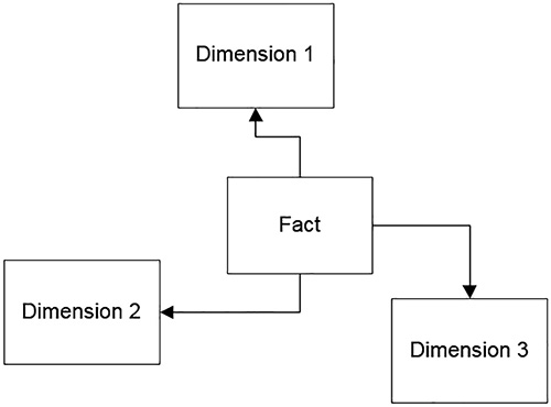
In some cases, a dimension links to other dimensions forming what is referred to as a snowflake schema, though ideally there is one join between fact and dimension. The concept of a star schema is that there is one central table that contains measurements (called a fact table) that needs to be reported on (typically the goal is to perform some aggregate), and a set of foreign key values that link to tables of values that the data can be summarized by (called dimensions). One such example in the WideWorldImportersDW is the Fact.[Order] table, shown in Listing 1-13.

LISTING 1-13 Columns in the Fact.Order table in WideWorldImportersDW

Click here to view code image

---

CREATE TABLE Fact.[Order]
(
   [Order Key] bigint IDENTITY(1,1) NOT NULL,
   [City Key] int NOT NULL,
   [Customer Key] int NOT NULL,
   [Stock Item Key] int NOT NULL,
   [Order Date Key] date NOT NULL,
   [Picked Date Key] date NULL,
   [Salesperson Key] int NOT NULL,
   [Picker Key] int NULL,
   [WWI Order ID] int NOT NULL,
   [WWI Backorder ID] int NULL,
   [Description] nvarchar(100) NOT NULL,
   [Package] nvarchar(50) NOT NULL,
   [Quantity] int NOT NULL,
   [Unit Price] decimal(18, 2) NOT NULL,
   [Tax Rate] decimal(18, 3) NOT NULL,
   [Total Excluding Tax] decimal(18, 2) NOT NULL,
   [Tax Amount] decimal(18, 2) NOT NULL,
   [Total Including Tax] decimal(18, 2) NOT NULL,
   [Lineage Key] int NOT NULL
);

---

Breaking this table down, the [Order Key] column is a surrogate key. Column: [City Key] down to [Picker Key] are dimension keys, or dimension foreign key references. The cardinality of the dimension compared to the fact table is generally very low. You could have millions of fact rows, but as few as 2 dimension rows. There are techniques used to combine dimensions, but the most germane point to our discussion of columnstore indexes is that dimensions are lower cardinality tables with factors that one might group the data. Sometimes in data warehouses, FOREIGN KEY constraints are implemented, and sometimes not. Having them in the database when querying can be helpful, because they provide guidance to tools and the optimizer. Having them on during loading can hinder load performance.

Columns from [WWI BackorderID] to [Package] are referred to as degenerate dimensions, which means they are at, or are nearly at, the cardinality of the row and are more often used for finding a row in the table, rather than for grouping data.

Columns from [Quantity] down to [Total Including Tax] as called measures. These are the values that a person writing a query applies math to. Many measures are additive, meaning you can sum the values (such as [Quantity] in this example, and others are not, such as [Tax Rate]. If you add a 10 percent tax rate to a 10 percent tax rate, you don’t get 20 percent, no matter your political affiliations.

The [Lineage Key] is used to track details of where data comes from during loads. The table Integration.Lineage contains information about what was loaded and when. In Listing 1-14, is the basic code for two dimensions that relate to the Fact.Orders table.

LISTING 1-14 Columns in the Customer and Date dimensions in WideWorldImportersDW

Click here to view code image

---

CREATE TABLE Dimension.Customer
(
   [Customer Key] int NOT NULL,
   [WWI Customer ID] int NOT NULL,
   [Customer] nvarchar(100) NOT NULL,
   [Bill To Customer] nvarchar(100) NOT NULL,
   [Category] nvarchar(50) NOT NULL,
   [Buying Group] nvarchar(50) NOT NULL,
   [Primary Contact] nvarchar(50) NOT NULL,
   [Postal Code] nvarchar(10) NOT NULL,
   [Valid From] datetime2(7) NOT NULL,
   [Valid To] datetime2(7) NOT NULL,
   [Lineage Key] int NOT NULL
);
CREATE TABLE Dimension.Date(
   Date date NOT NULL,
   [Day Number] int NOT NULL,
   [Day] nvarchar(10) NOT NULL,
   [Month] nvarchar(10) NOT NULL,
   [Short Month] nvarchar(3) NOT NULL,
   [Calendar Month Number] int NOT NULL,
   [Calendar Month Label] nvarchar(20) NOT NULL,
   [Calendar Year] int NOT NULL,
   [Calendar Year Label] nvarchar(10) NOT NULL,
   [Fiscal Month Number] int NOT NULL,
   [Fiscal Month Label] nvarchar(20) NOT NULL,
   [Fiscal Year] int NOT NULL,
   [Fiscal Year Label] nvarchar(10) NOT NULL,
   [ISO Week Number] int NOT NULL
);

---

We won’t go into too much detail about all of these columns in the tables. But, the [Customer Key] and the Date columns are the columns that are referenced from the fact table. In the Dimensions.Customer table, the [Valid From] and [Valid To] columns set up a slowly changing dimension, where you could have multiple copies of the same customer over time, as attributes change. There are no examples of having multiple versions of a customer in the sample database, and it would not change our indexing example either.

All of the other columns in the dimensions (other than [Lineage Key], which provides the same sort of information as for the fact) can be used to group data in queries. Because the WideWorldImporterDW database starts out configured for examples, we can begin by dropping the columnstore index that is initially on all of the fact tables.

Click here to view code image

DROP INDEX [CCX_Fact_Order] ON [Fact].[Order];

The table starts out with indexes on all of the foreign keys, as well as primary keys on the dimension keys that the query uses. Perform the following query (there are 231,412 rows in the Fact.[Order] table), which you likely note runs pretty quickly without the columnstore index):

Click here to view code image

SELECT Customer.Category, Date.[Calendar Month Number],
        COUNT(*) AS SalesCount,
        SUM([Total Excluding Tax]) as SalesTotal
FROM   Fact.[Order]
         JOIN Dimension.Date
            ON Date.Date = [Order].[Order Date Key]
         JOIN Dimension.Customer
            ON Customer.[Customer Key] = [Order].[Customer Key]
GROUP BY Customer.Category, Date.[Calendar Month Number]
ORDER BY Category, Date.[Calendar Month Number], SalesCount, SalesTotal;

The plan for this query, shown in Figure 1-27 is complicated by the cost of scanning the table, which pushes the query to use parallelism, even on my VM. The largest cost is the table scan of the heap structure that was left after removing the clustered columnstore index.

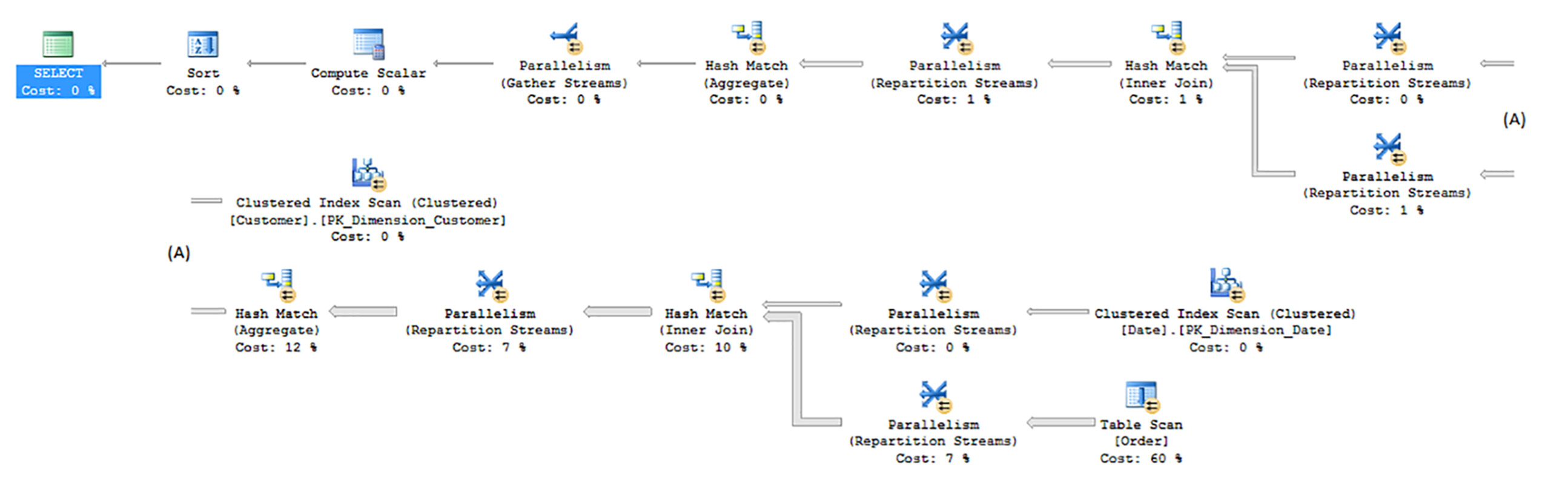
Figure 1-27 has the following output:

Click here to view code image

Table 'Customer'. Scan count 3, logical reads 40, physical reads 0, read-ahead reads 0,
lob logical reads 0, lob physical reads 0,

lob read-ahead reads 0.

Table 'Date'. Scan count 3, logical reads 79, physical reads 0, read-ahead reads 0, lob
logical reads 0, lob physical reads 0,

lob read-ahead reads 0.

Table 'Order'. Scan count 7, logical reads 5908, physical reads 0, read-ahead reads 0,
lob logical reads 0, lob physical reads 0,

lob read-ahead reads 0.

Table 'Workfile'. Scan count 0, logical reads 0, physical reads 0, read-ahead reads 0,
lob logical reads 0, lob physical reads 0,

lob read-ahead reads 0.

Table 'Worktable'. Scan count 0, logical reads 0, physical reads 0, read-ahead reads 0,
lob logical reads 0, lob physical reads 0,

lob read-ahead reads 0.

CPU time = 344 ms,  elapsed time = 276 ms.

Most of the plan is typical, as you often see Hash Match operators when joining two larger sets of data, which could not realistically be ordered in the same order as one another. Even with the smallish table structure for the fact table, there are 5908 logical reads (which is the same number of reads if it scanned the entire table once).

Prior to columnstore indexes, a suggested index to help this query would have been to use a covering index to cover the needs of this query so you didn’t have to touch any data other than the query needed. The optimizer suggested such an index for our query:

Click here to view code image

CREATE NONCLUSTERED INDEX SpecificQuery ON [Fact].[Order] ([Customer Key])
INCLUDE ([Order Date Key],[Total Excluding Tax]);

After adding this suggested index, the plan for this query is very similar, without the parallelism, and instead of a Table Scan operator that is 60 percent of the cost, there is an index scan that is 23 percent. The logical reads are reduced to 871 instead of 5908. The processing still takes around 300 ms, and actually took a bit longer than the full table scan versions at times. The problem with indexes that are tailored to specific queries is, if you want to add another column to your query, this index stops being of value. Columnstore indexes basically give you great aggregate and scan performance for most of the combinations of attributes you might consider without custom pre-planning.

Now, add the clustered columnstore index back to the table.

Click here to view code image

CREATE CLUSTERED COLUMNSTORE INDEX [CCX_Fact_Order] ON [Fact].[Order];

As the name clustered implies, this changes the internal structure of the table to be the columnar structures. We did not remove any of the rowstore indexes, and we review why you would or would not want to use both in tandem in section later in this chapter entitled “Design standard non-clustered indexes in conjunction with clustered columnstore indexes”.

The row locator for the rowstore indexes has been changed from the physical location in the heap, to the position in the columnstore structure (the row group, and the position in the row group). It is a bit more complex than this, and if you want more information, Niko Neugebauer has a great article about it here: http://www.nikoport.com/2015/09/06/columnstore-indexes-part-65-clustered-columnstore-improvements-in-sql-server-2016/.

For nearly all data warehousing applications, the clustered columnstore is a useful structure for fact tables when the table is large enough. Since the main copy of the data is compressed, you can see very large space savings, even having the table be 10 percent of the original size. Couple this with the usual stability of data in a data warehouse, with minimal changes to historical data, make the clustered columnstore typically ideal. Only cases where something does not work, like one of the data types that were mentioned in the introductory section (varchar(max) or nvarchar(max), for example) would you likely want to consider using a non-clustered columnstore index.

Whether or not a clustered columnstore index will be useful with a dimension will come down to how it is used. If the joins in your queries do not use a Nested Loop operator, there is a good chance it could be useful.

Perform the query again, and check the plan shown in Figure 1-28, which shows a tremendous difference:

Figure 1-28 has the following output:

Click here to view code image

Table 'Order'. Scan count 1, logical reads 0, physical reads 0, read-ahead reads 0, lob
logical reads 256, lob physical reads 0,

lob read-ahead reads 0.

Table 'Order'. Segment reads 4, segment skipped 0.

Table 'Worktable'. Scan count 0, logical reads 0, physical reads 0, read-ahead reads 0,
lob logical reads 0, lob physical reads 0,

lob read-ahead reads 0.

Table 'Customer'. Scan count 1, logical reads 15, physical reads 0, read-ahead reads 0,
lob logical reads 0, lob physical reads 0,

lob read-ahead reads 0.

Table 'Date'. Scan count 1, logical reads 28, physical reads 0, read-ahead reads 0, lob
logical reads 0, lob physical reads 0,

lob read-ahead reads 0.

CPU time = 15 ms,  elapsed time = 65 ms.

The logical reads are down to 256 in the lob reads for the segments, since the column segments are stored in a form of large varbinary storage. Note, too, that it took just 68ms rather than 286.

One thing that makes columnstore indexes better for queries such as those found in data warehouses is batch execution mode. When the query processor is scanning data in the columnstore index, it is possible for it to process rows in chunks of 900 rows at a time, rather than one row at a time in the typical row execution mode. Figure 1-29 displays the tool tip from hovering over the Columnstore Index Scan operator from Figure 1-28. The third and fourth lines down show you the estimated and actual execution mode. Batch execution mode can provide great performance improvements.

Finally, just for comparison, let us drop the clustered columnstore index, and add a non-clustered columnstore index. When you are unable to use a clustered one due to some limitation, non-clustered columnstore indexes are just as useful to your queries, but the base table data is not compressed, giving you less overall value.

In our demo, include all of the columns except for [Lineage ID] and [Description], which have no real analytic value to our user:

Click here to view code image

CREATE NONCLUSTERED COLUMNSTORE INDEX [NCCX_Fact_Order] ON [Fact].[Order] (
       [Order Key] ,[City Key] ,[Customer Key] ,[Stock Item Key]
      ,[Order Date Key] ,[Picked Date Key] ,[Salesperson Key] ,[Picker Key]
      ,[WWI Order ID],[WWI Backorder ID],[Package]
      ,[Quantity],[Unit Price],[Tax Rate],[Total Excluding Tax]
      ,[Tax Amount],[Total Including Tax]);

Executing the query one more time, the plan looks exactly like the query did previously, other than it is using a non-clustered columnstore operator rather than a clustered one. The number of reads go up slightly in comparison to the clustered example, but not tremendously. The beauty of the columnstore indexes however is how well they adapt to the queries you are executing. Check the plan and IO/time statistics for the following query, that adds in a new grouping criteria, and a few additional aggregates:

Click here to view code image

SELECT Customer.Category, Date.[Calendar Year],
        Date.[Calendar Month Number],
        COUNT(*) as SalesCount,
        SUM([Total Excluding Tax]) AS SalesTotal,
        AVG([Total Including Tax]) AS AvgWithTaxTotal,
        MAX(Date.Date) AS MaxOrderDate
FROM   Fact.[Order]
         JOIN Dimension.Date
            ON Date.Date = [Order].[Order Date Key]
         JOIN Dimension.Customer
            ON Customer.[Customer Key] = [Order].[Customer Key]
GROUP BY Customer.Category, Date.[Calendar Year], Date.[Calendar Month Number]
ORDER BY Category, Date.[Calendar Month Number], SalesCount, SalesTotal;

You should see very little change, including the time required to perform the query. This ability to cover many analytical indexing needs is what truly makes the columnstore indexes a major difference when building data warehouse applications. Hence, both the clustered and non-clustered columnstore indexes can be used to greatly improve your data warehouse loads, and in a later section, we review some of the differences.

By applying a non-clustered columnstore index to the table you wish to do real-time analytics on, you can enable tremendous performances with little additional query tuning. And depending on your concurrency needs, you can apply a few settings to tune how the columnstore index is maintained.

Columnstore indexes can be used to help greatly enhance reporting that accesses an OLTP database directly, certainly when paired with concurrency techniques that we cover in Chapter 3. Generally speaking, a few questions need to be considered: “How many reporting queries do you need to support?” and “How flexible does the reporting need to be?”

If, for example, the report is one, fairly rigid report that uses an index with included columns to cover the needs of that specific query could be better. But if the same table supports multiple reports, and particularly if there needs to be multiple indexes to support analytics, a columnstore index is a better tool.

In the WideWorldImporters database, there are a few examples of tables that have a non-clustered columnstore index, such as the OrderLines table, the abbreviated DDL of which is shown in Listing 1-15.

LISTING 1-15 Abbreviated structure of the WideWorldImporters.Sales.InvoiceLines table with non-clustered columnstore index

Click here to view code image

---

CREATE TABLE Sales.InvoiceLines
(
    InvoiceLineID int NOT NULL,
    InvoiceID int NOT NULL,
    StockItemID int NOT NULL,
    Description nvarchar(100) NOT NULL,
    PackageTypeID int NOT NULL,
    Quantity int NOT NULL,
    UnitPrice decimal(18, 2) NULL,
    TaxRate decimal(18, 3) NOT NULL,
    TaxAmount decimal(18, 2) NOT NULL,
    LineProfit decimal(18, 2) NOT NULL,
    ExtendedPrice decimal(18, 2) NOT NULL,
    LastEditedBy int NOT NULL,
    LastEditedWhen datetime2(7) NOT NULL,
 CONSTRAINT PK_Sales_InvoiceLines PRIMARY KEY
              CLUSTERED ( InvoiceLineID )
 );
--Not shown: FOREIGN KEY constraints, indexes other than the PK

CREATE NONCLUSTERED COLUMNSTORE INDEX NCCX_Sales_OrderLines ON Sales.OrderLines
(
    OrderID,
    StockItemID,
    Description,
    Quantity,
    UnitPrice,
    PickedQuantity
) ON USERDATA;

---

Now, if you are reporting on the columns that are included in the columnstore index, only the columnstore index is used. The needs of the OLTP (generally finding and operating on just a few rows), are served from the typical rowstore indexes. There are a few additional ways to improve the utilization and impact of the columnstore index on the overall performance of the table, which we examine in the following sections:

Targeting analytically valuable columns only in columnstore

Delaying adding rows to compressed rowgroups

Using filtered non-clustered columnstore indexes to target hot data

Hence there is a setting that lets you control the amount of time the data stays in the deltastore. The setting is: COMPRESSION_DELAY, and the units are minutes. This says that the data stays in the delta rowgroup for at least a certain number of minutes. The setting is added to the CREATE COLUMNSTORE INDEX statement, as seen in Listing 1-16.

LISTING 1-16 Changing the non-clustered columnstore index to have COMPRESSION_DELAY = 5 minutes

Click here to view code image

---

CREATE NONCLUSTERED COLUMNSTORE INDEX NCCX_Sales_OrderLines ON Sales.OrderLines
(
         OrderID,
         StockItemID,
         Description,
         Quantity,
         UnitPrice,
         PickedQuantity
) WITH (DROP_EXISTING = ON, COMPRESSION_DELAY = 5) ON USERDATA;

---

Now, in this case, say the PickedQuantity is important to the analytics you are trying to perform, but it is updated several times in the first 5 minutes (on average) after the row has been created. This ensures that the modifications happens in the deltastore, and as such does not end up wasting space in a compressed rowgroup being deleted and added over and over.

LISTING 1-17 Base structure of the Sales.Orders Table

Click here to view code image

---

CREATE TABLE Sales.Orders
(
    OrderID int NOT NULL,
    CustomerID int NOT NULL,
    SalespersonPersonID int NOT NULL,
    PickedByPersonID int NULL,
    ContactPersonID int NOT NULL,
    BackorderOrderID int NULL,
    OrderDate date NOT NULL,
    ExpectedDeliveryDate date NOT NULL,
    CustomerPurchaseOrderNumber nvarchar(20) NULL,
    IsUndersupplyBackordered bit NOT NULL,
    Comments nvarchar(max) NULL,
    DeliveryInstructions nvarchar(max) NULL,
    InternalComments nvarchar(max) NULL,
    PickingCompletedWhen datetime2(7) NULL,
    LastEditedBy int NOT NULL,
    LastEditedWhen datetime2(7) NOT NULL,
    CONSTRAINT PK_Sales_Orders PRIMARY KEY CLUSTERED
    (
       OrderID ASC
    )
);

---

One could then, applying a few of the principles we have mentioned in these sections, choose only the columns we are interested in, though we should not need to add a compression delay for this particular case since once the PickedByPersonID is set, we are saying the data is complete.

So we might set up:

Click here to view code image

CREATE NONCLUSTERED COLUMNSTORE INDEX NCCI_Orders ON Sales.Orders
(
      PickedByPersonId,
      SalespersonPersonID,
      OrderDate,
      PickingCompletedWhen
)
WHERE PickedByPersonId IS NOT NULL;

One additional thing you can do, if you need your reporting to span the cold and hot data, and that is to cluster your data on the key that is use for the filtering. So in this case, if you clustered your table by PickedByPersonId, the optimizer would easily be able to split the set for your queries. This could seem counter to the advice given earlier about clustering keys and it generally is. However, in some cases this could make a big difference if the reporting is critical. It is covered in more detail by Sunil Agarwal in his blog here (https://blogs.msdn.microsoft.com/sqlserverstorageengine/2016/03/06/real-time-operational-analytics-filtered-nonclustered-columnstore-index-ncci/) when he suggested using the a column with a domain of order status values in his example to cluster on, even though it has only 6 values and the table itself has millions.

Columnstore Indexes Great for working with large data sets, particularly for aggregation. Not great for looking up a single row, as the index is not ordered

Clustered Compresses the table to greatly reduce memory and disk footprint of data.

Nonclustered Addition to typical table structure, ideal when the columns included cover the needs of the query.

Rowstore Indexes Best used for seeking a row, or a set of rows in order.

Clustered Physically reorders table’s data in an order that is helpful. Useful for the primary access path where you fetch rows along with the rest of the row data, or for scanning data in a given order.

Nonclustered Structure best used for finding a single row. Not great for scanning unless all of the data needed is in the index keys, or is in included in the leaf pages of the index.

If you have worked with columnstore indexes in SQL Server 2012 or 2014, it is necessary to change how you think about using these indexes. In 2012, SQL Server only had read only non-clustered columnstore indexes, and to modify the data in the index (and any of the rows in the table), the index needed to be dropped and completely rebuilt. In 2014, read/write clustered columnstore indexes were added, but there was no way to have a rowstore index on the same table with them. When you needed to fetch a single row, the query processor needed to scan the entire table. If your ETL did many updates or deletes, the operation was costly. So for many applications, sticking with the drop and recreating a non-clustered index made sense.

In SQL Server 2016, the version that you are studying for in this exam, both types of columnstore indexes are read/write, and both allow you to have complimentary rowstore indexes. In this section, we focus on adding non-clustered indexes to your clustered columnstore indexes, which in the previous section we have established as generally the best practice for data warehousing situations, mostly fact tables, and possibly very large dimensions. The columnstore indexes are there to aid in analytical queries, but there are a few other needs to consider.

To demonstrate, begin by making a copy of the Fact.Sale table in the WideWorldImportersDW database, and adding a clustered columnstore index.

Click here to view code image

SELECT *
INTO   Fact.SaleBase
FROM   Fact.Sale;

CREATE CLUSTERED COLUMNSTORE INDEX CColumnsStore ON Fact.SaleBase;

You see that if you perform an aggregation query, the columnstore index is used, and the performance is stellar:

Click here to view code image

SELECT Date.[Fiscal Year], Customer.Category,  Sum(Quantity) as NumSales
FROM   Fact.SaleBase
         JOIN Dimension.Customer
            on Customer.[Customer Key] = SaleBase.[Customer Key]
         JOIN Dimension.Date
            ON Date.Date = SaleBase.[Invoice Date Key]
GROUP BY Date.[Fiscal Year], Customer.Category
ORDER BY Date.[Fiscal Year], Customer.Category;

And the plan is shown in Figure 1-30.

Figure 1-30 has the following output:

Click here to view code image

Table 'Worktable'. Scan count 0, logical reads 0, physical reads 0, read-ahead reads 0,
lob logical reads 0, lob physical reads 0,

lob read-ahead reads 0.

Table 'Customer'. Scan count 1, logical reads 15, physical reads 0, read-ahead reads 0,
lob logical reads 0, lob physical reads 0,

lob read-ahead reads 0.

Table 'Date'. Scan count 1, logical reads 28, physical reads 0, read-ahead reads 0, lob
logical reads 0, lob physical reads 0,

lob read-ahead reads 0.

CPU time = 15 ms,  elapsed time = 22 ms.

What is likely unexpected is what happens when filtering on a single value in a column not yet referenced by adding to the statement the following WHERE clause (a common operation when doing ETL where data can change):

Click here to view code image

WHERE SaleBase.[Sale Key] = 26974

The plan changes to something that looks better, but actually takes more time and considerably more IO as seen in Figure 1-31.

Figure 1-31 has the following output:

Click here to view code image

Table 'SaleBase'. Scan count 1, logical reads 0, physical reads 0, read-ahead reads 0,
lob logical reads 347, lob physical reads 0,

lob read-ahead reads 0.

Table 'SaleBase'. Segment reads 1, segment skipped 0.

Table 'Worktable'. Scan count 0, logical reads 0, physical reads 0, read-ahead reads 0,
lob logical reads 0, lob physical reads 0,

lob read-ahead reads 0.

Table 'Date'. Scan count 0, logical reads 2, physical reads 0, read-ahead reads 0, lob
logical reads 0, lob physical reads 0,

lob read-ahead reads 0.

Table 'Customer'. Scan count 0, logical reads 2, physical reads 0, read-ahead reads 0,
lob logical reads 0, lob physical reads 0,

lob read-ahead reads 0.

CPU time = 0 ms,  elapsed time = 40 ms.

Note that now the major cost is spent in the Columnstore Scan operator, which isn’t surprising since the query processor has to touch all of the rows in the table; for the column segment for the [Sale Key] in any case. This cost isn’t too much in this very small fact table (less than 300,000 rows), but it is very telling that you have an issue if you’re needing to fetch rows one at a time for some reason, either to update data, or delete a row.

So next we add indexes to the table for any cases where you want to access rows one at a time. Examples in the Fact.SaleBase table are columns like the surrogate key: [Sale Key], and the degenerate key: [WWI Invoice ID]. Other uses of indexes might be for filtering date ranges, or foreign key indexes when you want to get all rows of a given related dimension, depending on the cardinality of the relationship. For example, let’s add two indexes:

Click here to view code image

CREATE UNIQUE INDEX [Sale Key] ON Fact.SaleBase ([Sale Key]);
CREATE INDEX [WWI Invoice ID] ON Fact.SaleBase ([WWI Invoice ID]);

The [Sale Key] index is the surrogate key for the fact table, so it is unique, while the [WWI Invoice ID] is for the entire order, and the grain of the table is one row per invoice line item.

Now perform the query with the WHERE clause and you see the plan has changed to what you would desire for a single-row lookup, as you can see in Figure 1-32.

Figure 1-32 has the following output:

Click here to view code image

Table 'Date'. Scan count 0, logical reads 2, physical reads 0, read-ahead reads 0, lob
logical reads 0, lob physical reads 0,

lob read-ahead reads 0.

Table 'Customer'. Scan count 0, logical reads 2, physical reads 0, read-ahead reads 0,
lob logical reads 0, lob physical reads 0,

lob read-ahead reads 0.

Table 'SaleBase'. Scan count 1, logical reads 3, physical reads 0, read-ahead reads 0,
lob logical reads 186, lob physical reads 0,

lob read-ahead reads 0.

Table 'SaleBase'. Segment reads 1, segment skipped 0.

CPU time = 0 ms,  elapsed time = 30 ms.

Now, while you never aggregate just a row at a time, other than perhaps in development, when you go to update a single row in the table during ETL, the operation of finding the rows is not cost prohibitive.

You need to decide whether to wait for the tuple mover to handle your structure, force the tuple mover to perform, or just rebuild your indexes, depending on the urgency of your needs. If this is a nightly-loaded data warehouse and you have the time, you want to just use REBUILD, but if it is a more active system, you want to check the configuration of the index and do a REORGANIZE. We look at a few examples in this section.

There are a few ways that data is loaded into a columnstore:

Bulk Load Into a Clustered Columnstore Different from bulk loading data into a rowstore table, you can load bulk amounts of data into a clustered columnstore index by using an INSERT...SELECT ... FROM <TableName> WITH (TABLOCK) statement.

Other Batch Operations Loading data where you don’t meet the requirements of the Bulk Load pattern.

For each of the examples, use a pared-down version of the Fact.Sale table named Fact.SaleLimited, as shown in Listing 1-18

LISTING 1-18 Fact table code to be used for this section

Click here to view code image

---

.CREATE TABLE [Fact].[SaleLimited](
       [City Key] [int] NOT NULL,
             [Customer Key] [int] NOT NULL,
       [Bill To Customer Key] [int] NOT NULL,
       [Stock Item Key] [int] NOT NULL,
       [Invoice Date Key] [date] NOT NULL,
       [Delivery Date Key] [date] NULL,
       [Salesperson Key] [int] NOT NULL,
       [WWI Invoice ID] [int] NOT NULL,
       [Description] [nvarchar](100) NOT NULL,
       [Package] [nvarchar](50) NOT NULL,
       [Quantity] [int] NOT NULL
);

---

Click here to view code image

CREATE CLUSTERED COLUMNSTORE INDEX [CColumnStore] ON [Fact].[SaleLimited];

Next, load some data. The WITH (TABLOCK) allows this statement to run in parallel (for more information, the following blog has more details: https://blogs.msdn.microsoft.com/sqlcat/2016/07/21/real-world-parallel-insert-what-else-you-need-to-know/), so you could end up with more or less deltastores on your system:

Click here to view code image

INSERT INTO [Fact].[SaleLimited] WITH (TABLOCK)
     ([City Key], [Customer Key],  [Bill To Customer Key], [Stock Item Key],
      [Invoice Date Key], [Delivery Date Key],[Salesperson Key],
      [WWI Invoice ID], [Description], [Package], [Quantity])
SELECT TOP (100000) [City Key], [Customer Key],  [Bill To Customer Key],
          [Stock Item Key], [Invoice Date Key], [Delivery Date Key],[Salesperson Key],
          [WWI Invoice ID], [Description], [Package], [Quantity]
FROM Fact.Sale
GO 3 --run this statement 3 times

Next, go and look at the information from the DMV sys.dm_db_column_store_row_group_physical_stats, which gives you information about the physical characteristics of the rowgroups in your columnstore index. The query in Listing 1-19 is used throughout these maintenance sections to view the physical state of the columnstore indexes.

LISTING 1-19 Query on sys.dm_db_column_store_row_group_physical_stats to see state of columnstore indexes

Click here to view code image

---

SELECT state_desc, total_rows, deleted_rows,
       transition_to_compressed_state_desc as transition
FROM sys.dm_db_column_store_row_group_physical_stats
WHERE object_id  = OBJECT_ID('Fact.SaleLimited');

---

The output of this query, right after execution is:

Click here to view code image

state_desc      total_rows deleted_rows transition
--------------- ---------- ------------ ------------------------------
OPEN            150000     0            NULL
OPEN            150000     0            NULL

Two deltastore rowgroups were created, since there are two processors in my VM, and the bulk insert performs in parallel. If the VM had 8 processors, there could have been as many as 8 groups created. Since the total_rows column value is less than the 1048576 rows that is optimum, executing simple ALTER INDEX REORGANIZE does not change anything. The transition column tells you what triggered the row group to transition to a compressed state. There are other good bits of information not shown here, like the trim_reason that tells you why less than the expected maximum number of rows are in the rowgroup.

However, if you are not going to be adding any additional rows, you can force the tuple mover to compress these rowgroups by executing:

Click here to view code image

ALTER INDEX CColumnStore ON Fact.SaleLimited REORGANIZE
                                WITH (COMPRESS_ALL_ROW_GROUPS = ON);

Then you see:

Click here to view code image

state_desc      total_rows deleted_rows transition
--------------- ---------- ------------ ------------------------------
COMPRESSED      150000     0            REORG_FORCED
COMPRESSED      150000     0            REORG_FORCED
TOMBSTONE       150000     0            NULL
TOMBSTONE       150000     0            NULL

The two deltastore rowgroups have been compressed, and have then been tombstoned. When and whether you want to do these tasks largely depends on the type of table. For an OLTP table, where data is being loaded constantly, it may not be advantageous to reorganize the table, particularly if you are rapidly reaching the million row point. Of course, it is possible that you want to run the reorganize prior to a large reporting task. For a data warehouse table that is loaded periodically, you want to either rebuild or reorganize, depending on time allotted, and how many UPDATE and DELETE operations have occurred. Once you have compressed filegroups, things happen automatically.

Forcing the tuple mover to start by running REORGANIZE has the process combine the two compressed row groups, as the larger the number of rows in the rowgroup, up to the maximum, is better.

Click here to view code image

ALTER INDEX CColumnStore ON Fact.SaleLimited REORGANIZE;

Now check the structure of the columnstore index:

Click here to view code image

state_desc      total_rows deleted_rows transition
--------------- ---------- ------------ ------------------------------
COMPRESSED      300000     0            MERGE
TOMBSTONE       150000     0            NULL
TOMBSTONE       150000     0            NULL

Note, if you directly bulk insert 102400 or more rows, the data goes directly into compressed rowgroups as rows are being added. To show what happens when you bulk load at least the minimum number of rows, perform:

Click here to view code image

TRUNCATE TABLE Fact.SaleLimited;
GO
INSERT INTO [Fact].[SaleLimited] WITH (TABLOCK)
     ([City Key], [Customer Key],  [Bill To Customer Key], [Stock Item Key],
      [Invoice Date Key], [Delivery Date Key],[Salesperson Key],
      [WWI Invoice ID], [Description], [Package], [Quantity])
SELECT TOP (102400) [City Key], [Customer Key],  [Bill To Customer Key],
          [Stock Item Key], [Invoice Date Key], [Delivery Date Key],[Salesperson Key],
          [WWI Invoice ID], [Description], [Package], [Quantity]
FROM Fact.Sale
OPTION (MAXDOP 1); --not in parallel
GO 3

You now see three compressed rowgroups in the output of the Listing 1-19 query. This is better for actually using the row groups immediately, but not as efficient as having them all in the same rowgroup:

Click here to view code image

state_desc      total_rows deleted_rows transition
--------------- ---------- ------------ ------------------------------
COMPRESSED      102400     0            BULKLOAD
COMPRESSED      102400     0            BULKLOAD
COMPRESSED      102400     0            BULKLOAD

Perform ALTER INDEX REORGANIZE, and these three rowgroups are combined into just 1.

Click here to view code image

state_desc      total_rows deleted_rows transition
--------------- ---------- ------------ ------------------------------
COMPRESSED      307200     0            MERGE
TOMBSTONE       102400     0            NULL
TOMBSTONE       102400     0            NULL
TOMBSTONE       102400     0            NULL

Using ALTER INDEX...REBUILD skips directly to having all of the rowgroups compressed in the best fashion possible, much like dropping and recreating the index, but it is an offline process just like initially recreating the index. This is true, even a minimal number of rows, as in this example:

Click here to view code image

TRUNCATE TABLE Fact.SaleLimited;
INSERT INTO [Fact].[SaleLimited] WITH (TABLOCK)
([City Key],     [Customer Key],
                 [Bill To Customer Key], [Stock Item Key],
                 [Invoice Date Key], [Delivery Date Key],[Salesperson Key],
                 [WWI Invoice ID], [Description], [Package], [Quantity])

SELECT TOP (5000) [City Key],     [Customer Key],
                 [Bill To Customer Key], [Stock Item Key],
                 [Invoice Date Key], [Delivery Date Key],[Salesperson Key],
                 [WWI Invoice ID], [Description], [Package], [Quantity]

FROM Fact.Sale;

Then rebuild the index:

Click here to view code image

ALTER INDEX [CColumnStore] ON [Fact].[SaleLimited] REBUILD;

And there is a compressed rowgroup with only 5000 rows:

Click here to view code image

state_desc      total_rows deleted_rows transition
--------------- ---------- ------------ ------------------------------
COMPRESSED      5000       0            INDEX_BUILD

Click here to view code image

TRUNCATE TABLE Fact.SaleLimited;
INSERT INTO [Fact].[SaleLimited]
([City Key],     [Customer Key],
                 [Bill To Customer Key], [Stock Item Key],
                 [Invoice Date Key], [Delivery Date Key],[Salesperson Key],
                 [WWI Invoice ID], [Description], [Package], [Quantity])

SELECT TOP (100000 ) [City Key],      [Customer Key],
                  [Bill To Customer Key], [Stock Item Key],
                  [Invoice Date Key], [Delivery Date Key],[Salesperson Key],
                  [WWI Invoice ID], [Description], [Package], [Quantity]

FROM Fact.Sale;
ALTER INDEX [CColumnStore] ON [Fact].[SaleLimited] REBUILD;

Now the structure looks like:

Click here to view code image

state_desc      total_rows deleted_rows transition
--------------- ---------- ------------ ------------------------------
COMPRESSED      100000     0            INDEX_BUILD

Then delete some data:

Click here to view code image

DELETE FROM Fact.SaleLimited
WHERE  [Customer Key] = 21;

You now see what is sometimes thought of as fragmentation showing up. There are still 100000 rows in the rowgroup, but 135 rows are marked as deleted. As this number grows, the rowgroup becomes less and less useful:

Click here to view code image

state_desc      total_rows deleted_rows transition
--------------- ---------- ------------ ------------------------------
COMPRESSED      100000     135          INDEX_BUILD

Next, update some data:

UPDATE Fact.SaleLimited
SET    [Customer Key] = 35
WHERE  [Customer Key] = 22;

Looking at the structure, you can now see that we have more deleted rows, and a new delta rowgroup for the inserted versions of the updated rows.

Click here to view code image

state_desc      total_rows deleted_rows transition
--------------- ---------- ------------ ------------------------------
OPEN            98         0            NULL
COMPRESSED      100000     233          INDEX_BUILD

From here, there are three choices. Wait for the tuple mover to deal with this situation, though maybe not if more data isn’t loaded. REBUILD, or REORGANIZE using the COMPRESS_ALL_ROW_GROUPS option as done in the previous section.

The steps done here are the same for non-clustered and clustered columnstore indexes, but the non-clustered version does not update the deleted_rows column, whereas the clustered does. Columnstore indexes are wonderful for many things, but they are definitely tuned for large quantities of data, particularly when the automated processes work after more than a million rows are inserted. This, plus the fact that they can get fragmented from just simple INSERT, UPDATE, and DELETE statements means you certainly want to keep up with how the load from your processes is affecting the rowgroups.

Columnstore Indexes Defragmentation https://msdn.microsoft.com/en-us/library/dn935013.aspx. Details on what fragments columnstore indexes, and links to Sunil Agarwal’s blogs on the topics as well.

Part 36 of Niko Neugebauer’s blog series on clustered columnstore indexes http://www.nikoport.com/2014/07/29/clustered-columnstore-indexes-part-36-maintenance-solutions-for-columnstore/. Of course, the other many sections of his series on columnstore indexes are useful reading as well.

An excellent blog on the Tuple Mover on the Rusanu Consulting Blog, mentioned by Sunil Agarwal http://rusanu.com/2013/12/02/sql-server-clustered-columnstore-tuple-mover/.

Columnstore Data Loading https://msdn.microsoft.com/en-us/library/dn935008.aspx Covers how data is loaded into the columnstore index, and how this affects the need to maintain your indexes.

Understanding what normalization means is essential to the process of matching the needs of the user to the needs of the query optimizer and processor. The normal forms are very much about eliminated duplication in your structures to enhance data integrity,

SQL Server provides you as a user with a tremendous number of data types, not all of which you need for any given design. Match the data type you need to the requirements the user provides or, if no prescribed size is provided, to a size that is large enough to handle any reasonable value, but not so large as to allow unnecessarily large values. For example: nvarchar(3) for a person’s name, too small, nvarchar(max) far too large. nvarchar(50) is probably more than you ever need, but not so large that it is ridiculous.

Dynamic Data Masking can be added to the declaration for a column in the table create statement to mask data from database principals that do not have the UNMASK privilege in the database. There are several functions you can use to mask data.

The clustered index of a table is a very important choice, as the key columns are used in all other rowstore indexes. The greater percentage of your queries can use the clustered index for seek operations to answer queries the better. The best clustered indexes are small in size, never changing, and monotonically increasing. A small clustering key size reduces the size of all nonclustered indexes; never changing values eliminates updates to non-clustered indexes; and monotonically increasing lets data be inserted at the end of the physical structures.

An essential tool for designing indexes is the query plan. Use the graphical versions from the UI, or one of the SET SHOWPLAN commands to get a textual version of the estimated plan, or SET STATISTICS PROFILE ON for a textual version of the actual plan. Adding indexes without any real knowledge of how they are used often ends up creating useless indexes (something that is touched on in Chapter 4.)

Index key columns can total 900 bytes or less for a clustered index, and up to 1700 bytes for a non-clustered index.

There is only one clustered index, which makes it very important to choose what to put in the clustered index wisely for two reasons:

The data pages of the table are ordered by the clustering key

All non-clustered indexes use the clustering key for their row locators

Providing summarized/denormalized data to the client by DML based automated means can be achieved using an indexed view.

Columnstore indexes are specifically built for analytic purposes and typically need to be coupled with rowstore indexes to allow searches on a single row, unless you extremely rarely need to fetch a single row.

Clustered columnstore indexes change your table’s storage and compress your data considerably, reducing the amount of IO needed to perform queries on very large data sets. Nonclustered columnstore indexes can be added to a rowstore table to allow real-time analytics.

In columnstore indexes, DELETE operations just mark compressed rows as deleted, and UPDATE operations mark the row to be updated deleted and perform and INSERT. Both INSERT operations add rows to a deltastore rowgroup. Unless your table is very active, you need to perform maintenance on your table using ALTER INDEX REORGANIZE or ALTER INDEX REBUILD to get the most out of your columnstore indexes, as the background tuple mover moves rows when there are 1048576 rows in the deltastore rowgroup.

You are taking over the table design for the invoicing system for a toy shop. The requirements state “Wingtip Toys want to track their customer’s basic information, the orders they have placed for one or more products, and how much they have paid for each product on the order. The price of a toy can change for every order.”

In the database, you see the following tables, with accompanying definitions:

Customer People and companies that have purchase toys from the shop

CustomerOwnedToys Toys that we know a customer owns

InvoiceItem The bill for the toys that a customer has purchased

Product The list of products that Wingtip Toys sells.

What are the potential issues with the design, based solely on the table names?

The original designer had created a column in the Customer table named: nickname, allowing you to store a name a person would prefer to be called. For example, a person named William might prefer to be called Bill, and Mariusz Wolodzko could prefer to be called “Captain Awesome.” The data type for this column is int, and you realize that int is not really a desirable data type for storing a text value. You have the following five different data types that you are deciding from:

1. varchar (100)

2. nvarchar(50)

3. nvarchar(Max)

4. char(120)

5. varbinary(100)

For each type, evaluate in terms of A. Ability to store the data B. Appropriateness of the data type to meet the specified requirements.

Once the database has been created, the following query is written:

Click here to view code image

SELECT StockItemID, StockItemName, SupplierID, ColorID, UnitPackageID,
       OuterPackageID, Brand, Size
FROM   Examples.Product
WHERE  UnitPackageId = 9;

And the plan for this query is shown in Figure 1-33:

From the information given, can you decide if adding either of the following indexes improves the query?

CREATE INDEX UnitPackageId ON Examples.Product (UnitPackageId);

CREATE INDEX UnitPackageIdPlus ON Examples.Product (UnitPackageId) INCLUDE (StockItemID, StockItemName, SupplierID, ColorID, OuterPackageID, Brand, Size);

Finally, in your review, you see the following table with over 5 million rows in it:

Click here to view code image

CREATE TABLE Sales.InvoiceItemFact
(
    InvoiceItemFactId int NOT NULL
          IDENTITY CONSTRAINT PKInvoiceItemFact PRIMARY KEY,
    ProductDimId int NOT NULL,
    CustomerDimId int NOT NULL,
    DateDimId int NOT NULL,
    SalesAmount money NOT NULL,
    SalesQuantity decimal(10,4)

);

There is also a table named Sales.ProductDim and Sales.CustomerDim, that contain data about the customer and product associated with the sale. Do all of the indexes work with the existing PRIMARY KEY constraint’s index? For queries that aggregate a lot of data in the table, do the indexes help?

CREATE INDEX ProductDimId ON Sales.InvoiceItemFact (ProductDimId);

CREATE NONCLUSTERED COLUMNSTORE INDEX NCColumnstore ON Sales.InvoiceItemFact (InvoiceItemFactId, ProductDimId, CustomerDimId, DateDimId, SalesAmount, SalesQuantity);

CREATE CLUSTERED COLUMNSTORE INDEX CColumnstore ON Sales.InvoiceItemFact;

There are several concerns in the design as given, both in terms of meeting the requirements given and basic normalization considerations. In terms of requirements, there is a table named CustomerOwnedToys, specifying a feature that was not requested by the customer. The normalization problem comes with just having an InvoiceItem table without a table named Invoice. This causes the columns to need to repeat information about the order that was placed. There was one answer included to possibly throw you off. “The price of a toy can change for every order” seems to indicate that we need a ProductPrice table. However, the requirements strictly ask “how much they have paid for each product on the order”.

A column for a person’s nickname is a typical need, and clearly int is not the proper solution. Let’s look at each type mentioned, in terms of A. Ability to store the data, and B. Appropriateness of the data type to meet the specified requirements.

1. varchar (100)

A. Since this is an ASCII type, it is acceptable for storing simple character data. However, real names contain special characters. It is best to use a Unicode type for names

B. 100 characters of string data is likely too long of a string for name data, the width of text on this page is approximately 80 characters wide. If you are going to allow 100 characters in a column, usage should never cut it off. Since it is variably sized, it does not waste space, making it efficient enough.

2. nvarchar(50)

A. This is a Unicode type, and as such it should handle any text.

B. 50 characters is a typical length that people set names to be. Since it is variably sized, it does not waste space, making it efficient enough.

3. nvarchar(Max)

A. This is a Unicode type, and as such it should handle any text.

B. Much like other larger strings, this is too large of a string for a name at over 1 million characters. Some designers simply use nvarchar(max) because it is easy, and since it is variably sized, technically no less efficient than any other nvarchar type. However, this is generally not the best practice that is desirable.

4. char(120)

A. Since this is an ASCII type, it is acceptable for storing simple character data. However, real names contain special characters. It is best to use a Unicode type for names.

B. 120 characters is too long, and in this case, since it is not variable sized, space is typically wasted when storing a short string. Even if using a compression setting (not covered in this exam), the string appears padded in all uses, which is not optimal.

5. varbinary(100)

A. If you assumed that this would not work, you were incorrect. While it is definitely not the most efficient way to store a string, the following CAST expression results in a Unicode string of N’Bill’: CAST (0x420069006C006C00 as nvarchar(100)).

B. Clearly this is not optimum way of storing a string. However, this is something that could have been done in very old systems to give binary comparisons. Using a binary collation provides the same properties in modern versions of SQL Server.

Given the query we have been provided on the Examples.Product table, without any data to look at, it is not possible to be sure that either index that we are provided with gives any benefit (for example, what if the table had 1 row? The size of the line from the Clustered Index Scan to the SELECT operator is very thin. It also isn’t stated if an index already exists on the UnitPackage column.) However, so this isn’t just a trick question, let’s assume that there is data in the table, there is not an index on UnitPackageId, and some data was returned from the query.

CREATE INDEX UnitPackageId ON Examples.Product (UnitPackageId); This index has the least likelihood between the two to provide benefit. For it to be useful, there needs to be a lot of rows that don’t match, and just a few that do, based on the statistics of the table. Because of the necessity of a Key Lookup operator to fetch additional columns that are not in the index, the value of this index has to be great to outweigh the costs.

CREATE INDEX UnitPackageIdPlus ON Examples.Product (UnitPackageId) INCLUDE (StockItemID, StockItemName, SupplierID, ColorID, OuterPackageID, Brand, Size); There is no guarantee that this index tremendously improves the query, since we are not sure if there are columns in the table that are not included but the index, but since the index key matches the WHERE clause, and the INCLUDE columns match the SELECT clause, it can almost certainly be of some value to the query.

Finally, there were a few indexes that were to be applied to a fact table in a dimensional design.

All indexes listed work with the existing PRIMARY KEY constraint index.

CREATE INDEX ProductDimId ON Sales.InvoiceItemFact (ProductDimId); This index is generally only be useful for queries only return a ProductDimId, such as counting the number of orders per ProductDimId. Generally, this is not a great, general-purpose index.

CREATE NONCLUSTERED COLUMNSTORE INDEX NCColumnstore ON Sales.InvoiceItemFact (InvoiceItemFactId, ProductDimId, CustomerDimId, DateDimId, SalesAmount, SalesQuantity); Almost all queries that do analytical queries on the Sales.InvoiceItemFact table can benefit from this index. However, the non-clustered columnstore index is generally more appropriate for OLTP tables, where you want a minimal overhead for the OLTP users, and no change to the base table structures.

CREATE CLUSTERED COLUMNSTORE INDEX CColumnstore ON Sales.InvoiceItemFact; This is the best choice of index from the list. It compresses the base data in the table to make the IO impact the smallest for all queries. It works nicely with the PRIMARY KEY constraint index to allow singleton updates/seeks as needed for ETL and simple queries also.