
Choosing the right datatype seems so easy and straightforward, but many times I see it done incorrectly. The most basic decision—what type you use to store your data in—will have repercussions on your applications and data for years to come. Thus, choosing the appropriate datatype is paramount. It is also hard to change after the fact—in other words, once you implement it, you might be stuck with it for quite a while.
In this chapter, we’ll take a look at all of the Oracle basic datatypes available and discuss how they are implemented and when each might be appropriate to use. We won’t examine user-defined datatypes as they’re simply compound objects derived from the built-in Oracle datatypes. We’ll investigate what happens when you use the wrong datatype for the job—or even just the wrong parameters to the datatype (length, precision, scale, and so on). By the end of this chapter, you’ll have an understanding of the types available to you, how they’re implemented, when to use each type, and, as important, why using the right type for the job is key.
An Overview of Oracle Datatypes
CHAR: A fixed-length character string that will be blank padded with spaces to its maximum length. A non-null CHAR(10) will always contain 10 bytes of information using the default National Language Support (NLS) settings. We will cover NLS implications in more detail shortly. A CHAR field may store up to 2000 bytes of information.
NCHAR: A fixed-length character string that contains UNICODE formatted data. Unicode is a character-encoding standard developed by the Unicode Consortium with the aim of providing a universal way of encoding characters of any language, regardless of the computer system or platform being used. The NCHAR type allows a database to contain data in two different character sets: the CHAR type and NCHAR type use the database’s character set and the national character set, respectively. A non-null NCHAR(10) will always contain 10 characters of information (note that it differs from the CHAR type in this respect). An NCHAR field may store up to 2000 bytes of information.
VARCHAR2: Also currently synonymous with VARCHAR. This is a variable-length character string that differs from the CHAR type in that it is not blank padded to its maximum length. A VARCHAR2(10) may contain between 0 and 10 bytes of information using the default NLS settings. A VARCHAR2 may store up to 4000 bytes of information. Starting with Oracle 12c, a VARCHAR2 can be configured to store up to 32,767 bytes of information (see the “Extended Datatypes” section in this chapter for further details).
NVARCHAR2: A variable length character string that contains UNICODE formatted data. An NVARCHAR2(10) may contain between 0 and 10 characters of information. An NVARCHAR2 may store up to 4,000 bytes of information. Starting with Oracle 12c, an NVARCHAR2 can be configured to store up to 32,767 bytes of information (see the “Extended Datatypes” section in this chapter for further details).
RAW: A variable-length binary datatype, meaning that no character set conversion will take place on data stored in this datatype. It is considered a string of binary bytes of information that will simply be stored by the database. A RAW may store up to 2000 bytes of information. Starting with Oracle 12c, a RAW can be configured to store up to 32,767 bytes of information (see the “Extended Datatypes” section in this chapter for further details).
NUMBER: This datatype is capable of storing numbers with up to 38 digits of precision. These numbers may vary between 1.0x10(–130) and up to but not including 1.0x10(126). Each number is stored in a variable-length field that varies between 0 bytes (for NULL) and 22 bytes. Oracle NUMBER types are very precise—much more so than normal FLOAT and DOUBLE types found in many programming languages.
BINARY_FLOAT : This is a 32-bit single-precision floating-point number. It can support at least six digits of precision and will consume 5 bytes of storage on disk.
BINARY_DOUBLE: This is a 64-bit double-precision floating-point number. It can support at least 15 digits of precision and will consume 9 bytes of storage on disk.
LONG: This type is capable of storing up to 2GB of character data (2 gigabytes, not characters, as each character may take multiple bytes in a multibyte character set). LONG types have many restrictions (I’ll discuss later) that are provided for backward compatibility, so it is strongly recommended you do not use this type in new applications. When possible, convert from LONG to CLOB types in existing applications.
LONG RAW: The LONG RAW type is capable of storing up to 2GB of binary information. For the same reasons as noted for LONGs, it is recommended you use the BLOB type in all future development and, when possible, in existing applications as well.
DATE : This is a fixed-width 7-byte date/time datatype. It will always contain the seven attributes of the century, the year within the century, the month, the day of the month, the hour, the minute, and the second.
TIMESTAMP : This is a fixed-width 7- or 11-byte date/time datatype (depending on the precision). It differs from the DATE datatype in that it may contain fractional seconds; up to nine digits to the right of the decimal point may be preserved for TIMESTAMPs with fractional seconds.
TIMESTAMP WITH TIME ZONE: This is a fixed-width 13-byte date/time datatype, but it also provides for TIME ZONE support. Additional information regarding the time zone is stored with the TIMESTAMP in the data, so the TIME ZONE originally inserted is preserved with the data.
TIMESTAMP WITH LOCAL TIME ZONE: This is a fixed-width 7- or 11-byte date/time datatype (depending on the precision), similar to the TIMESTAMP; however, it is time zone sensitive. Upon modification in the database, the TIME ZONE supplied with the data is consulted, and the date/time component is normalized to the local database time zone. So, if you were to insert a date/time using the time zone US/Pacific and the database time zone was US/Eastern, the final date/time information would be converted to the Eastern time zone and stored as a TIMESTAMP. Upon retrieval, the TIMESTAMP stored in the database would be converted to the time in the session’s time zone.
INTERVAL YEAR TO MONTH: This is a fixed-width 5-byte datatype that stores a duration of time, in this case as a number of years and months. You may use intervals in date arithmetic to add or subtract a period of time from a DATE or the TIMESTAMP types.
INTERVAL DAY TO SECOND : This is a fixed-width 11-byte datatype that stores a duration of time, in this case as a number of days and hours, minutes, and seconds, optionally with up to nine digits of fractional seconds.
BLOB: This datatype permits for the storage of up to (4 gigabytes – 1) * (database block size) bytes of data in Oracle. BLOBs contain “binary” information that is not subject to character set conversion. This would be an appropriate type in which to store a spreadsheet, a word processing document, image files, and the like.
CLOB: This datatype permits for the storage of up to (4 gigabytes –1) * (database block size) bytes of data in Oracle. CLOBs contain information that is subject to character set conversion. This would be an appropriate type in which to store large plain text information. Note that I said large plain text information; this datatype would not be appropriate if your plain text data is 4000 bytes or less—for that you would want to use the VARCHAR2 datatype.
NCLOB: This datatype permits for the storage of up to (4 gigabytes – 1) * (database block size) bytes of data in Oracle. NCLOB s store information encoded in the national character set of the database and are subject to character set conversions just as CLOBs are.
BFILE : This datatype permits you to store an Oracle directory object (a pointer to an operating system directory) and a file name in a database column and to read this file. This effectively allows you to access operating system files available on the database server in a read-only fashion, as if they were stored in the database table itself.
ROWID: A ROWID is effectively a 10-byte address of a row in a database. Sufficient information is encoded in the ROWID to locate the row on disk, as well as identify the object the ROWID points to (the table and so on).
UROWID: A UROWID is a universal ROWID and is used for tables—such as IOTs and tables accessed via gateways to heterogeneous databases—that do not have fixed ROWIDs. The UROWID is a representation of the primary key value of the row and hence will vary in size depending on the object to which it points.
JSON: New with Oracle 21c is the JSON datatype. You can now store JSON data natively in the database in a binary format.
Many types are apparently missing from the preceding list, such as INT, INTEGER, SMALLINT, FLOAT, REAL, and others. These types are actually implemented on top of one of the base types in the preceding list—that is, they are synonyms for the native Oracle type. Additionally, datatypes such as XMLType, SYS.ANYTYPE, and SDO_GEOMETRY are not listed because we will not cover them in this book. They are complex object types comprising a collection of attributes along with the methods (functions) that operate on those attributes. They are made up of the basic datatypes listed previously and are not truly datatypes in the conventional sense, but rather an implementation, a set of functionality, that you may make use of in your applications.
Now, let’s take a closer look at these basic datatypes.
Character and Binary String Types
The character datatypes in Oracle are CHAR, VARCHAR2, and their “N” variants. The CHAR and NCHAR can store up to 2000 bytes of text. The VARCHAR2 and NVARCHAR2 can store up to 4000 bytes of information.
Starting with Oracle 12c, VARCHAR2, NVARCHAR2, and RAW datatypes can be configured to store up to 32,767 bytes of information. Extended datatypes are not enabled by default; therefore, unless explicitly configured, the maximum size is still 4000 bytes for VARCHAR2 and NVARCHAR2 datatypes and 2000 bytes for RAW. See the “Extended Datatypes” section later in this chapter for more details.
The US7ASCII character set is the ASCII standard representation of 128 characters. It uses the low 7 bits of a byte to represent these 128 characters.
The WE8MSWIN1252 character set is a Western European character set capable of representing the 128 ASCII characters as well as 128 extended characters, using all 8 bits of a byte.
Before we get into the details of CHAR, VARCHAR2, and their “N” variants, it would benefit us to get a cursory understanding of what these different character sets mean to us.
NLS Overview
As stated earlier, NLS stands for National Language Support . NLS is a very powerful feature of the database, but one that is often not as well understood as it should be. NLS controls many aspects of our data. For example, it controls how data is sorted and whether we see commas and a single period in a number (e.g., 1,000,000.01) or many periods and a single comma (e.g., 1.000.000,01). But most important, it controls the following:
Encoding of the textual data as stored persistently on disk
Transparent conversion of data from character set to character set
It is this transparent part that confuses people the most—it is so transparent, you cannot even really see it happening. Let’s look at a small example.
Suppose you are storing 8-bit data in a WE8MSWIN1252 character set in your database, but you have some clients that connect using a 7-bit character set such as US7ASCII. These clients are not expecting 8-bit data and need to have the data from the database converted into something they can use. While this sounds wonderful, if you are not aware of it taking place, then you might well find that your data loses characters over time as the characters that are not available in US7ASCII are translated into some character that is. This is due to the character set translation taking place. In short, if you retrieve data from the database in character set 1, convert it to character set 2, and then insert it back (reversing the process), there is a very good chance that you have materially modified the data. Character set conversion is typically a process that will change the data, and you are usually mapping a large set of characters (in this example, the set of 8-bit characters) into a smaller set (that of the 7-bit characters). This is a lossy conversion —the characters get modified because it is quite simply not possible to represent every character. But this conversion must take place. If the database is storing data in a single-byte character set but the client (say, a Java application, since the Java language uses Unicode) expects it in a multibyte representation, then it must be converted simply so the client application can work with it.
If you do this example yourself and do not see the preceding output, make sure your terminal client software is using a UTF-8 character set itself. Otherwise, it might be translating the characters when printing to the screen! A common terminal emulator for UNIX will typically be 7-bit ASCII. This affects both Windows and UNIX/Linux users alike. Make sure your terminal can display the characters.
where 97, 141, and 61 are the corresponding ASCII codes for the “a” character in decimal, octal, and hexadecimal notations. The returned datatype code of Typ=96 indicates a CHAR datatype (see the Oracle Database SQL Language Reference manual for a complete list of Oracle datatype codes and meanings).
Such warnings should be treated very seriously. If you were exporting this table with the goal of dropping the table and then using IMP to re-create it, you would find that all of your data in that table was now lowly 7-bit data! Beware the unintentional character set conversion.
The problem of unintentional character set conversion does not affect every tool, nor does it affect every tool in the same ways. For example, if you were to use the recommended Data Pump export/import process, you would discover that the export is always done in the character set of the database containing the data, regardless of the client’s NLS settings. This is because Data Pump runs in the database server itself; it is not a client-side tool at all. Similarly, Data Pump import will always convert the data in the file to be imported from the source database’s character set into the destination database’s character set—meaning that character set conversion is still possible with Data Pump (if the source and target databases have different character sets) but not in the same fashion as with the legacy EXP/IMP tools!
But also be aware that, in general, character set conversions are necessary. If clients are expecting data in a specific character set, it would be disastrous to send them the information in a different character set.
I highly encourage everyone to read through the Oracle Database Globalization Support Guide document. It covers NLS-related issues to a depth we will not here. Anyone creating applications that will be used around the globe (or even across international boundaries) needs to master the information contained in that document.
Now that we have a cursory understanding of character sets and the impact they will have on us, let’s take a look at the character string types provided by Oracle.
Character Strings
There are four basic character string types in Oracle, namely, CHAR, VARCHAR2, NCHAR, and NVARCHAR2. All of the strings are stored in the same format in Oracle. On the database block, they will have a leading length field of 1–3 bytes followed by the data; when they are NULL, they will be represented as a single-byte value of 0xFF.
Trailing NULL columns consume 0 bytes of storage in Oracle. This means that if the last column in a table is NULL, Oracle stores nothing for it. If the last two columns are both NULL, there will be nothing stored for either of them. But if any column after a NULL column in position is not null, then Oracle will use the null flag, described in this section, to indicate the missing value.
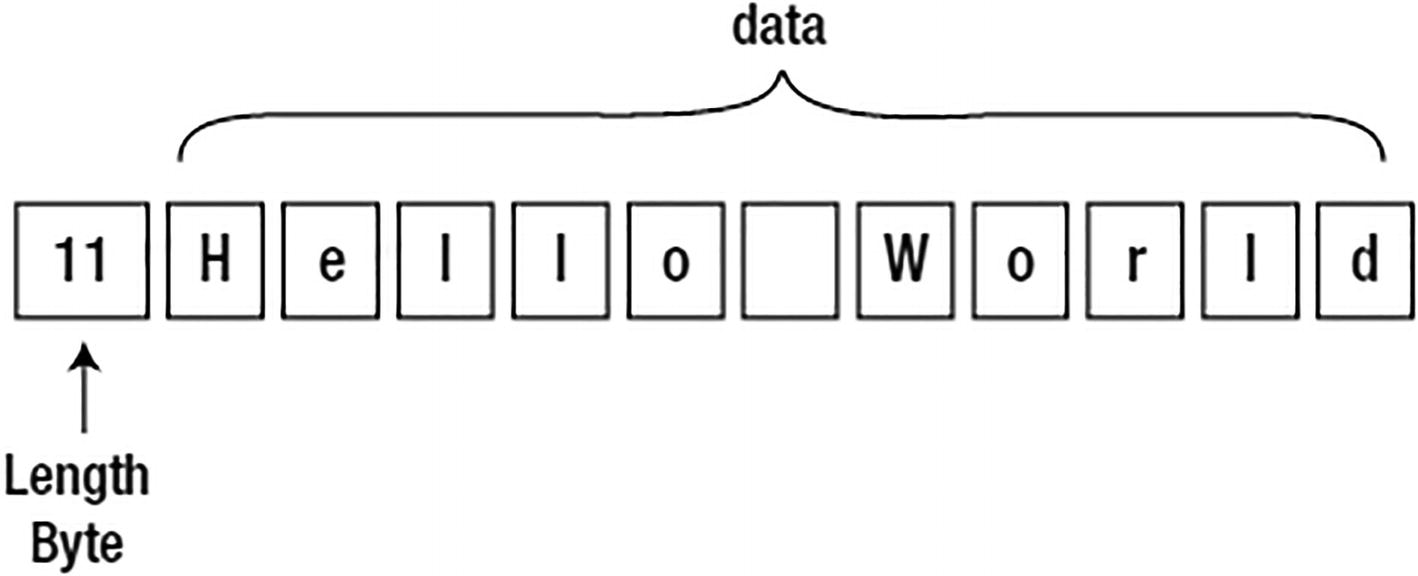
Hello World stored in a VARCHAR2(80)
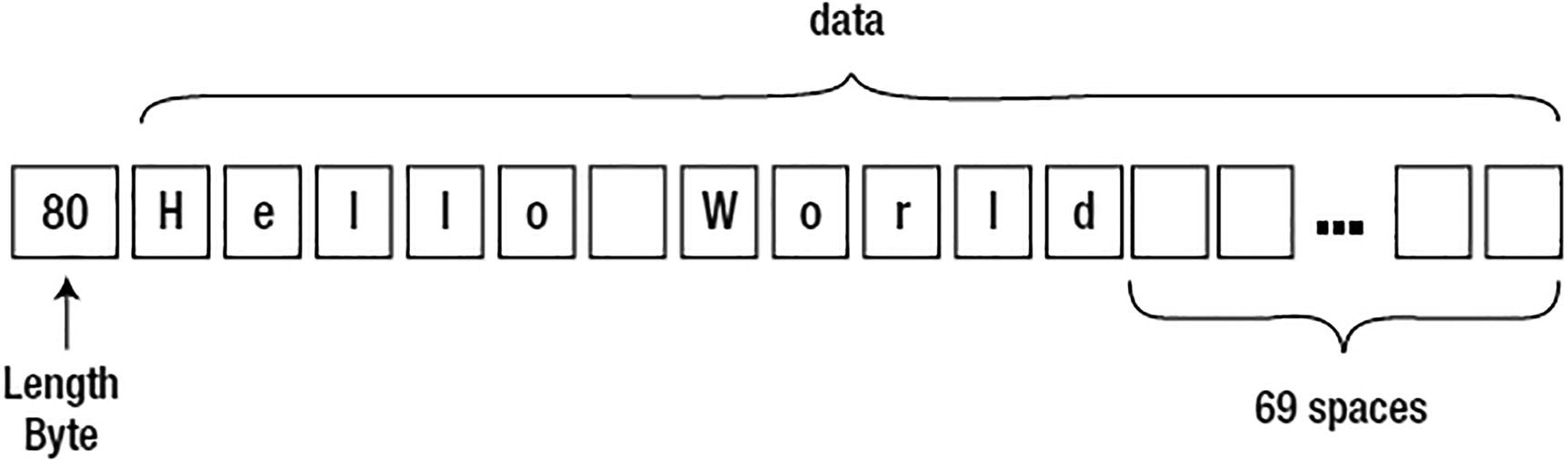
Hello World stored in a CHAR(80)
There are many ways to blank pad the VARCHAR2_COLUMN, such as using the CAST() function.
However, if you mix and match VARCHAR2 and CHAR, you’ll be running into this issue constantly. Not only that, but the developer is now having to consider the field width in their applications. If the developer opts for the RPAD() trick to convert the bind variable into something that will be comparable to the CHAR field (it is preferable, of course, to pad out the bind variable, rather than TRIM the database column, as applying the function TRIM to the column could easily make it impossible to use existing indexes on that column), they would have to be concerned with column length changes over time. If the size of the field changes, then the application is impacted, as it must change its field width.
It is for these reasons—the fixed-width storage, which tends to make the tables and related indexes much larger than normal, coupled with the bind variable issue—that I avoid the CHAR type in all circumstances. I cannot even make an argument for it in the case of the one-character field, because in that case it is really of no material difference. The VARCHAR2(1) and CHAR(1) are identical in all aspects. There is no compelling reason to use the CHAR type in that case, and to avoid any confusion, I “just say no,” even for the CHAR(1) field.
Character String Syntax
Four Basic String Types
String Type | <SIZE> |
|---|---|
VARCHAR2( <SIZE> <BYTE|CHAR> ) | A number between 1 and 4000 for up to 4000 bytes of storage. In the following section, we’ll examine in detail the differences and nuances of the BYTE vs. CHAR modifier in that clause. Starting with 12c, you can configure a VARCHAR2 to store up to 32,767 bytes of information. |
CHAR( <SIZE> <BYTE|CHAR> ) | A number between 1 and 2000 for up to 2000 bytes of storage. |
NVARCHAR2( <SIZE> ) | A number greater than 0 whose upper bound is dictated by your national character set. Starting with 12c, you can configure an NVARCHAR2 to store up to 32,767 bytes of information. |
NCHAR( <SIZE> ) | A number greater than 0 whose upper bound is dictated by your national character set. |
Bytes or Characters
In bytes: VARCHAR2(10 byte). This will support up to 10 bytes of data, which could be as few as two characters in a multibyte character set. Remember that bytes are not the same as characters in a multibyte character set!
In characters: VARCHAR2(10 char). This will support up to ten characters of data, which could be as much as 40 bytes of information. Furthermore, VARCHAR2(4000 CHAR) would theoretically support up to 4000 characters of data, but since a character string datatype in Oracle is limited to 4000 bytes, you might not be able to store that many characters. See the following for an example.
When using a multibyte character set such as UTF8, you would be well advised to use the CHAR modifier in the VARCHAR2/CHAR definition—that is, use VARCHAR2(80 CHAR), not VARCHAR2(80), since your intention is likely to define a column that can in fact store 80 characters of data. You may also use the session or system parameter NLS_LENGTH_SEMANTICS to change the default behavior from BYTE to CHAR. I do not recommend changing this setting at the system level; rather, use it as part of an ALTER SESSION setting in your database schema installation scripts. Any application that requires a database to have a specific set of NLS settings makes for an unfriendly application. Such applications generally cannot be installed into a database with other applications that do not desire these settings, but rely on the defaults to be in place.
One other important thing to remember is that the upper bound of the number of bytes stored in a VARCHAR2 is 4000. However, even if you specify VARCHAR2(4000 CHAR), you may not be able to fit 4000 characters into that field. In fact, you may be able to fit as few as 1000 characters in that field if all of the characters take 4 bytes to be represented in your chosen character set! Regarding the 4000-byte limit, starting with 12c, a VARCHAR2 can be configured to store up to 32,767 bytes of information.
VARCHAR2(1) is in bytes, not characters. We have a single Unicode character, but it won’t fit into a single byte.
As you migrate an application from a single-byte fixed-width character set to a multibyte character set, you might find that the text that once fit into your fields no longer does.
The reason for the second point is that a 20-character string in a single-byte character set is 20 bytes long and will absolutely fit into a VARCHAR2(20). However, a 20-character field could be as long as 80 bytes in a multibyte character set, and 20 Unicode characters may well not fit in 20 bytes. You might consider modifying your DDL to be VARCHAR2(20 CHAR) or using the NLS_LENGTH_SEMANTICS session parameter mentioned previously when running your DDL to create your tables.
That INSERT succeeded, and we can see that the LENGTH of the inserted data is one character—all of the character string functions work character-wise. So the length of the field is one character, but the LENGTHB (length in bytes) function shows it takes 2 bytes of storage, and the DUMP function shows us exactly what those bytes are. So, that example demonstrates one very common issue people encounter when using multibyte character sets, namely, that a VARCHAR2(N) doesn’t necessarily hold N characters, but rather N bytes.
The next example works on databases that do not have extended datatypes enabled.
And as you can see, they consume 4000 bytes of storage.
The “N” Variant
So, of what use are the NVARCHAR2 and NCHAR (for completeness)? They are used in systems where the need to manage and store multiple character sets arises. This typically happens in a database where the predominant character set is a single-byte fixed-width one (such as WE8MSWIN1252), but the need arises to maintain and store some multibyte data. There are many systems that have legacy data but need to support multibyte data for some new applications; likewise, there are systems that want the efficiency of a single-byte character set for most operations (string operations on a string that uses fixed-width characters are more efficient than on a string where each character may use a different number of bytes) but need the flexibility of multibyte data at some point.
Their text is stored and managed in the database’s national character set, not the default character set.
Their lengths are always provided in characters, whereas a CHAR/VARCHAR2 may specify either bytes or characters.
This makes the NCHAR and NVARCHAR types suitable for storing only multibyte data.
Binary Strings: RAW Types
Oracle supports the storage of binary data as well as text. Binary data is not subject to the character set conversions we discussed earlier with regard to the CHAR and VARCHAR2 types. Therefore, binary datatypes are not suitable for storing user-supplied text, but are suitable for storing encrypted information—encrypted data is not “text,” but a binary representation of the original text, word processing documents containing binary markup information, and so on. Any string of bytes that should not be considered by the database to be “text” (or any other base datatype such as a number, date, and so on) and that should not have character set conversion applied to it should be stored in a binary datatype.
The RAW type, which we focus on in this section, is suitable for storing RAW data up to 2000 bytes in size. Starting with 12c, you can configure a RAW to store up to 32,767 bytes of information.
The BLOB type, which supports binary data of much larger sizes. We’ll defer coverage of this until the “LOB Types” section later in the chapter.
The LONG RAW type, which is supported for backward compatibility and should not be considered for new applications.
The RAW type is much like the VARCHAR2 type in terms of storage on disk. The RAW type is a variable-length binary string, meaning that the table T just created, for example, may store anywhere from 0 to 16 bytes of binary data. It is not padded out like the CHAR type.
You can immediately note two things here. First, the RAW data looks like a character string. That is just how SQL*Plus retrieved and printed it; that is not how it is stored on disk. SQL*Plus cannot print arbitrary binary data on your screen, as that could have serious side effects on the display. Remember that binary data may include control characters such as a carriage return or linefeed—or maybe a Ctrl+G character that would cause your terminal to beep.
The RAW type may be indexed and used in predicates—it is as functional as any other datatype. However, you must take care to avoid unwanted implicit conversions, and you must be aware that they will occur.
HEXTORAW: To convert strings of hexadecimal characters to the RAW type
RAWTOHEX: To convert RAW strings to hexadecimal strings
Extended Datatypes
Refer to the Oracle Database Reference guide for complete details on implementing extended datatypes for all types of databases (single instance, container, RAC, and Data Guard Logical Standby).
Once you’ve modified the MAX_STRING_SIZE to EXTENDED, you cannot modify the value back to the default (of STANDARD). It’s a one-way change. If you need to switch back, you will have to perform a recovery to a point in time before the change was made—meaning you’ll need RMAN backups (taken prior to the change) or have the Flashback Database enabled. You can also take a Data Pump export from a database with extended datatypes enabled and import into a database without extended datatypes enabled with the caveat that any tables with extended columns will fail on the import.
You have no direct control over the LOB associated with the extended column. This means that you cannot manipulate the underlying LOB column with the DBMS_LOB package. Also, the internal LOB associated with the extended datatype column is not visible to you via DBA_TAB_COLUMNS or COL$.
The LOB segment and associated LOB index are always stored in the tablespace of the table that the extended datatype was created in. Following normal LOB storage rules, Oracle stores the first 4000 bytes inline within the table. Anything greater than 4000 bytes is stored in the LOB segment. If the tablespace that the LOB is created in is using Automatic Segment Space Management (ASSM), then the LOB is created as a SecureFiles LOB; otherwise, it is created as a BasicFiles LOB.
See the “LOB Types” section later in this chapter for a discussion on in-row storage and the technical aspects of SecureFiles and BasicFiles.
The prior examples demonstrate that you have more flexibility working with an extended datatype than you would if working directly with a LOB column. Therefore, if you have an application that deals with character data greater than 4000 bytes but less than or equal to 32,727 bytes, then you may want to consider using extended datatypes. Also, if you’re migrating from a non-Oracle database (that supports large character columns) to an Oracle database, the extended datatype feature will help make that migration easier, as you can now define large sizes for VARCHAR2, NVARCHAR2, and RAW columns natively in Oracle.
Number Types
NUMBER: The Oracle NUMBER type is capable of storing numbers with an extremely large degree of precision—38 digits of precision, in fact. The underlying data format is similar to a packed decimal representation. The Oracle NUMBER type is a variable-length format from 0 to 22 bytes in length. It is appropriate for storing any number as small as 10e-130 and numbers up to but not including 10e126. This is by far the most common NUMBER type in use today.
BINARY_FLOAT: This is an IEEE native single-precision floating-point number. On disk, it will consume 5 bytes of storage: 4 fixed bytes for the floating-point number and 1 length byte. It is capable of storing numbers in the range of ~ ± 1038.53 with six digits of precision.
BINARY_DOUBLE: This is an IEEE native double-precision floating-point number. On disk, it will consume 9 bytes of storage: 8 fixed bytes for the floating-point number and 1 length byte. It is capable of storing numbers in the range of ~ ± 10308.25 with 13 digits of precision.
The value in NUM_COL is equal to 123*1e20, and not the value we attempted to insert.
NUMBER Type Syntax and Usage
Precision, or the total number of digits: By default, the precision is 38 and has valid values in the range of 1 to 38. The character * may be used to represent 38 as well.
Scale, or the number of digits to the right of the decimal point: Valid values for the scale are –84 to 127, and its default value depends on whether or not the precision is specified. If no precision is specified, then the scale defaults to the maximum range. If a precision is specified, then the scale defaults to 0 (no digits to the right of the decimal point). So, for example, a column defined as NUMBER stores floating-point numbers (with decimal places), whereas a NUMBER(38) stores only integer data (no decimals), since the scale defaults to 0 in the second case.
So, you can use the precision to enforce some data integrity constraints. In this case, NUM_COL is a column that is not allowed to have more than five digits.
When you specify the scale of 2, at most three digits may be to the left of the decimal place and two to the right. Hence, that number does not fit. The NUMBER(5,2) column can hold all values between 999.99 and –999.99.
So, the precision dictates how many digits are permitted in the number after rounding, using the scale to determine how to round. The precision is an integrity constraint, whereas the scale is an edit.
We can see that as we added significant digits to X, the amount of storage required took increasingly more room. Every two significant digits added another byte of storage. But a number just one larger consistently took 2 bytes. When Oracle stores a number, it does so by storing as little as it can to represent that number. It does this by storing the significant digits, an exponent used to place the decimal place, and information regarding the sign of the number (positive or negative). So, the more significant digits a number contains, the more storage it consumes.
That last fact explains why it is useful to know that numbers are stored in varying width fields. When attempting to size a table (e.g., to figure out how much storage 1,000,000 rows would need in a table), you have to consider the NUMBER fields carefully. Will your numbers take 2 bytes or 20 bytes? What is the average size? This makes accurately sizing a table without representative test data very hard. You can get the worst-case size and the best-case size, but the real size will likely be some value in between.
BINARY_FLOAT/BINARY_DOUBLE Type Syntax and Usage
A floating-point number is a digital representation for a number in a certain subset of the rational numbers, and is often used to approximate an arbitrary real number on a computer. In particular, it represents an integer or fixed-point number (the significand or, informally, the mantissa) multiplied by a base (usually 2 in computers) to some integer power (the exponent). When the base is 2, it is the binary analogue of scientific notation (in base 10).
This is not a bug, this is the way IEEE floating-point numbers work. As a result, they are useful for a certain domain of problems, but definitely not for problems where dollars and cents count!
That is it. There are no options to these types whatsoever.
Non-native Number Types
NUMERIC(p,s): Maps exactly to a NUMBER(p,s). If p is not specified, it defaults to 38.
DECIMAL(p,s) or DEC(p,s): Maps exactly to a NUMBER(p,s). If p is not specified, it defaults to 38.
INTEGER or INT: Maps exactly to the NUMBER(38) type.
SMALLINT: Maps exactly to the NUMBER(38) type.
FLOAT(p): Maps to the NUMBER type.
DOUBLE PRECISION: Maps to the NUMBER type.
REAL: Maps to the NUMBER type.
When I say “syntactically supports,” I mean that a CREATE statement may use these datatypes, but under the covers they are all really the NUMBER type. There are precisely three native numeric formats. The use of any other numeric datatype is always mapped to the native Oracle NUMBER type.
Performance Considerations
In general, the Oracle NUMBER type is the best overall choice for most applications. However, there are performance implications associated with that type. The Oracle NUMBER type is a software datatype—it is implemented in the Oracle software itself. We cannot use native hardware operations to add two NUMBER types together, as it is emulated in the software. The floating-point types, however, do not have this implementation. When we add two floating-point numbers together, Oracle will use the hardware to perform the operation.
The floating-point numbers were an approximation of the number, with between 6 and 13 digits of precision. The answer from the NUMBER type is much more precise than from the floats. However, when you are performing data mining or complex numerical analysis of scientific data, this loss of precision is typically acceptable, and the performance gain to be had can be dramatic.
If you are interested in the gory details of floating-point arithmetic and the subsequent loss of precision, see https://docs.oracle.com/cd/E19957-01/806-3568/ncg_goldberg.html.
This implies that we may store our data very precisely, and when the need for raw speed arises, and the floating-point types significantly outperform the Oracle NUMBER type, we can use the CAST function to accomplish that goal.
Long Types
A LONG text type capable of storing 2GB of text. The text stored in the LONG type is subject to character set conversion, much like a VARCHAR2 or CHAR type.
A LONG RAW type capable of storing 2GB of raw binary data (data that is not subject to character set conversion).
The LONG types date back to version 6 of Oracle, when they were limited to 64KB of data. In version 7, they were enhanced to support up to 2GB of storage, but by the time version 8 was released, they were superseded by the LOB types, which we will discuss shortly.
Do not create a table with LONG columns. Use LOB columns (CLOB, NCLOB, BLOB) instead. LONG columns are supported only for backward compatibility.
Restrictions on LONG and LONG RAW Types
Long Types Compared to LOBs
LONG/LONG RAW Type | CLOB/BLOB Type |
|---|---|
You may have only one LONG or LONG RAW column per table. | You may have up to 1000 columns of CLOB or BLOB type per table. |
User-defined types may not be defined with attributes of type LONG/LONG RAW. | User-defined types may fully use CLOB and BLOB types. |
LONG types may not be referenced in the WHERE clause. | LOBs may be referenced in the WHERE clause, and a host of functions is supplied in the DBMS_LOB package to manipulate them. |
LONG types do not support distributed transactions. | LOBs do support distributed transactions. |
LONG types cannot be replicated using basic or advanced replication. | LOBs fully support replication. |
LONG columns cannot be in a GROUP BY, ORDER BY, or CONNECT BY or in a query that uses DISTINCT, UNIQUE, INTERSECT, MINUS, or UNION. | LOBs may appear in these clauses provided a function is applied to the LOB that converts it into a scalar SQL type (contains an atomic value) such as a VARCHAR2, NUMBER, or DATE. |
PL/SQL functions/procedures cannot accept an input of type LONG. | PL/SQL works fully with LOB types. |
SQL built-in functions cannot be used against LONG columns (e.g., SUBSTR). | SQL functions may be used against LOB types. |
You cannot use a LONG type in a CREATE TABLE AS SELECT statement. | LOBs support CREATE TABLE AS SELECT. |
You cannot use ALTER TABLE MOVE on a table containing LONG types. | You may move tables containing LOBs. |
As you can see, Table 12-2 presents quite a long list; there are many things you just cannot do when you have a LONG column in the table. For all new applications, do not even consider using the LONG type. Instead, use the appropriate LOB type. For existing applications, you should seriously consider converting the LONG type to the corresponding LOB type if you are hitting any of the restrictions in Table 12-2. Care has been taken to provide backward compatibility so that an application written for LONG types will work against the LOB type transparently.
It almost goes without saying that you should perform a full functionality test against your application(s) before modifying your production system from LONG to LOB types.
Coping with Legacy LONG Types
You’ve converted the first 4000 bytes of the TEXT column from LONG to VARCHAR2 and can now use a predicate on it. Using the same technique, you could implement your own INSTR, LIKE, and so forth for LONG types as well. In this book, I’ll only demonstrate how to get the substring of a LONG type.
Note that on line 2, we specify AUTHID CURRENT_USER . This makes the package run as the invoker, with all roles and grants in place. This is important for two reasons. First, we’d like the database security to not be subverted—this package will only return substrings of columns we (the invoker) are allowed to see. Specifically, that means this package is not vulnerable to SQL injection attacks—it is not running as the owner of the package but as the invoker. Second, we’d like to install this package once in the database and have its functionality available for all to use; using invoker rights allows us to do that. If we used the default security model of PL/SQL—definer rights—the package would run with the privileges of the owner of the package, meaning it would only be able to see data the owner of the package could see, which may not include the set of data the invoker is allowed to see.
The concept behind the function SUBSTR_OF is to take a query that selects at most one row and one column: the LONG value we are interested in. SUBSTR_OF will parse that query if needed, bind any inputs to it, and fetch the results programmatically, returning the necessary piece of the LONG value.
Using this same technique—that of processing the result of a query that returns a single row with a single LONG column in a function—you can implement your own INSTR, LIKE, and so on as needed.
This implementation works well on the LONG type, but will not work on LONG RAW types. LONG RAWs are not piecewise accessible (there is no COLUMN_VALUE_LONG_RAW function in DBMS_SQL). Fortunately, this is not too serious of a restriction since LONG RAWs are not used in the dictionary, and the need to “substring” so you can search on it is rare. If you do have a need to do so, however, you will not use PL/SQL unless the LONG RAW is 32KB or less, as there is simply no method for dealing with LONG RAWs over 32KB in PL/SQL itself. Java, C, C++, Visual Basic, or some other language would have to be used.
This would work well in an application that occasionally needs to work with a single LONG RAW value. You would not want to continuously do that, however, due to the amount of work involved. If you find yourself needing to resort to this technique frequently, you should definitely convert the LONG RAW to a BLOB once and be done with it.
Dates, Timestamps, and Interval Types
The native Oracle datatypes of DATE, TIMESTAMP, and INTERVAL are closely related. The DATE and TIMESTAMP types store fixed date/times with varying degrees of precision. The INTERVAL type is used to store an amount of time, such as “8 hours” or “30 days,” easily. The result of subtracting two timestamps might be an interval; the result of adding an interval of eight hours to a TIMESTAMP results in a new TIMESTAMP that is eight hours later.
The DATE datatype has been part of Oracle for many releases—as far back as my experience with Oracle goes, which means at least back to version 5 and probably before. The TIMESTAMP and INTERVAL types are relative newcomers to the scene by comparison. For this simple reason, you will find the DATE datatype to be the most prevalent type for storing date/time information. But many new applications are using the TIMESTAMP type for two reasons: it has support for fractions of seconds (the DATE type does not), and it has support for time zones (something the DATE type also does not have).
We’ll take a look at each type after discussing DATE/TIMESTAMP formats and their uses.
Formats
I am not going to attempt to cover all of the DATE, TIMESTAMP, and INTERVAL formats here. This is well covered in the Oracle Database SQL Language Reference manual, which is freely available to all. A wealth of formats is available to you, and a good understanding of what they are is vital. I strongly recommend that you investigate them.
To format the data on the way out of the database in a style that pleases you
To tell the database how to convert an input string into a DATE, TIMESTAMP, or INTERVAL
And that is all. The common misconception I’ve observed over the years is that the format used somehow affects what is stored on disk and how the data is actually saved. The format has no effect at all on how the data is stored. The format is only used to convert the single binary format used to store a DATE into a string or to convert a string into the single binary format that is used to store a DATE. The same is true for TIMESTAMPs and INTERVALs.
My advice on formats is simply this: use them. Use them when you send a string to the database that represents a DATE, TIMESTAMP, or INTERVAL. Do not rely on default date formats—defaults can and probably will at some point in the future be changed by someone.
Refer back to Chapter 1 for a really good security reason to never use TO_CHAR/TO_DATE without an explicit format. In that chapter, I described a SQL injection attack that was available to an end user simply because the developer forgot to use an explicit format. Additionally, performing date operations without using an explicit date format can and will lead to incorrect answers. In order to appreciate this, just tell me what date this string represents: ‘01-02-03’. Whatever you say it represents, I’ll tell you that you are wrong. Never rely on defaults!
is that Feb 1, 2010, or Feb 1, 1910? Either one is a valid value; you cannot just pick one to be correct.
This same discussion applies to data leaving the database. If you execute SELECT DATE_COLUMN FROM T and fetch that column into a string in your application, then you should apply an explicit date format to it. Whatever format your application is expecting should be explicitly applied there. Otherwise, at some point in the future when someone changes the default date format, your application may break or behave incorrectly.
Next, let’s look at the datatypes themselves in more detail.
DATE Type
The month and day bytes, the next two fields, are stored naturally, without any modification. So, June 25 used a month byte of 6 and a day byte of 25. The hour, minute, and second fields are stored in excess-1 notation, meaning we must subtract 1 from each component to see what time it really was. Hence, midnight is represented as 1,1,1 in the date field.
To truncate that date down to the year, all the database had to do was put 1s in the last 5 bytes—a very fast operation. We now have a sortable, comparable DATE field that is truncated to the year level, and we got it as efficiently as possible.
Adding or Subtracting Time from a DATE
Simply add a NUMBER to the DATE. Adding 1 to a DATE is a method to add one day. Adding 1/24 to a DATE therefore adds one hour, and so on.
You may use the INTERVAL type, as described shortly, to add units of time. INTERVAL types support two levels of granularity: years and months or days/hours/minutes/seconds. That is, you may have an interval of so many years and months or an interval of so many days, hours, minutes, and seconds.
Add months using the built-in ADD_MONTHS function. Since adding a month is generally not as simple as adding 28 to 31 days, a special purpose function was implemented to facilitate this.
Adding Time to a Date
Unit of Time | Operation | Description |
|---|---|---|
N seconds | DATE + n/24/60/60 DATE + n/86400 DATE + NUMTODSINTERVAL(n,'second') | There are 86,400 seconds in a day. Since adding 1 adds one day, adding 1/86400 adds one second to a date. I prefer the n/24/60/60 technique over the 1/86400 technique. They are equivalent. An even more readable method is to use the NUMTODSINTERVAL (number to day/second interval) to add N seconds. |
N minutes | DATE + n/24/60 DATE + n/1440 DATE + NUMTODSINTERVAL(n,'minute') | There are 1440 minutes in a day. Adding 1/1440 therefore adds one minute to a DATE. An even more readable method is to use the NUMTODSINTERVAL function. |
N hours | DATE + n/24 DATE + NUMTODSINTERVAL(n,'hour') | There are 24 hours in a day. Adding 1/24 therefore adds one hour to a DATE. An even more readable method is to use the NUMTODSINTERVAL function. |
N days | DATE + n | Simply add N to the DATE to add or subtract N days. |
N weeks | DATE + 7*n | A week is seven days, so just multiply 7 by the number of weeks to add or subtract. |
N months | ADD_MONTHS(DATE,n) DATE + NUMTOYMINTERVAL(n,'month') | You may use the ADD_MONTHS built-in function or add an interval of N months to the DATE. Please see the important caveat noted shortly regarding using month intervals with DATEs. |
N years | ADD_MONTHS(DATE,12*n) DATE + NUMTOYMINTERVAL(n,'year') | You may use the ADD_MONTHS built-in function with 12*n to add or subtract N years. Similar goals may be achieved with a year interval, but please see the important caveat noted shortly regarding using year intervals with dates. |
Use the NUMTODSINTERVAL built-in function to add hours, minutes, and seconds.
Add a simple number to add days.
Use the ADD_MONTHS built-in function to add months and years.
I do not recommend using the NUMTOYMINTERVAL function (to add months and years). The reason has to do with how the functions behave at the months’ end.
See how the result of adding one month to February 29, 2000, results in March 31, 2000? February 29 was the last day of that month so ADD_MONTHS returned the last day of the next month. Additionally, notice how adding one month to January 30, 2000 and 2001 results in the last day of February 2000 and 2001, respectively.
In my experience, this makes using a month interval in date arithmetic impossible in general. A similar issue arises with a year interval: adding one year to February 29, 2000, results in a runtime error because there is no February 29, 2001.
Getting the Difference Between Two DATEs
Now it is clear that there is 1 year, 15 days, 10 hours, 20 minutes, and 30 seconds between the two DATEs.
TIMESTAMP Type
The TIMESTAMP type is very much like the DATE, with the addition of support for fractional seconds and time zones. We’ll look at the TIMESTAMP type in the following three sections: one with regard to just the fractional second support but no time zone support, and the other two with regard to the two methods of storing the TIMESTAMP with time zone support.
TIMESTAMP
We can see the fractional seconds that were stored are there in the last 4 bytes. We used the DUMP function to inspect the data in HEX this time (base 16) so we could easily convert the 4 bytes into the decimal representation.
Adding or Subtracting Time to/from a TIMESTAMP
Using the function that returns an INTERVAL type preserved the fidelity of the TIMESTAMP. You will need to exercise caution when using TIMESTAMPs to avoid the implicit conversions. But bear in mind the caveat about adding intervals of months or years to a TIMESTAMP if the resulting day isn’t a valid date—the operation fails (adding one month to the last day in January will always fail if the month is added via an INTERVAL).
Getting the Difference Between Two TIMESTAMPs
I personally find this unacceptable. The fact is, though, that by the time you are displaying information with years and months, the fidelity of the TIMESTAMP is destroyed already. A year is not fixed in duration (it may be 365 or 366 days in length) and neither is a month. If you are displaying information with years and months, the loss of microseconds is not relevant; having the information displayed down to the second is more than sufficient at that point.
TIMESTAMP WITH TIME ZONE Type
Upon retrieval, the default TIMESTAMP WITH TIME ZONE format included the time zone information (I was on US Mountain Daylight Time when this was executed).
TIMESTAMP WITH TIME ZONEs store the data in whatever time zone was specified when the data was stored. The time zone becomes part of the data itself. Note how the TIMESTAMP with TIME ZONE stores two more bytes than the TIMESTAMP column. The trailing 2 bytes are used upon retrieval to properly adjust the TIMESTAMP value.
It is not my intention to cover all of the nuances of time zones here in this book; that is a topic well covered elsewhere. To that end, I’ll just point out that there is support for time zones in this datatype. This support is more relevant in applications today than ever before. In the distant past, applications were not nearly as global as they are now. In the days before widespread Internet use, applications were many times distributed and decentralized, and the time zone was implicitly based on where the server was located. Today, with large centralized systems being used by people worldwide, the need to track and use time zones is very relevant.
Since there is a three-hour time difference between those two time zones, even though they show the same time of 16:02:32.212, the interval reported is a three-hour difference. When performing TIMESTAMP arithmetic on TIMESTAMP WITH TIME ZONE types, Oracle automatically converts both types to UTC time first and then performs the operation.
TIMESTAMP WITH LOCAL TIME ZONE Type
DT: This column stored the date/time 27-FEB-2014 16:02:32. The time zone and fractional seconds are lost because we used the DATE type. No time zone conversions were performed at all. We stored the exact date/time inserted, but lost the time zone.
TS1: This column preserved the TIME ZONE information and was normalized to be in UTC with respect to that TIME ZONE. The inserted TIMESTAMP value was in the US/Pacific time zone, which at the time of this writing was eight hours off UTC. Therefore, the stored date/time was 28-FEB-2014 00:02:32. It advanced our input time by eight hours to make it UTC time, and it saved the time zone US/Pacific as the last 2 bytes so this data can be properly interpreted later.
TS2: This column is assumed to be in the database’s time zone, which is US/Mountain. Now, 16:02:32 US/Pacific is 17:02:32 US/Mountain, so that is what was stored in the bytes ...18,3,33... (excess-1 notation; remember to subtract 1).
The database would be able to show that information, but the TS2 column with the LOCAL TIME ZONE (the time zone of the database) shows the time in the database’s time zone, which is the assumed time zone for that column (and in fact all columns in this database with the LOCAL TIME ZONE). My database was in the US/Mountain time zone, so 16:02:32 US/Pacific on the way in is now displayed as 5:00 p.m. Mountain time on the way out.
You may get slightly different results if the date was stored when the Standard time zone was in effect and then retrieved when Daylight Savings time is in effect. The output in the prior example would show a two-hour difference instead of what you would intuitively think would be a one-hour difference. I only point this out to drive home the fact that time zone math is much more complex than it appears!
The TIMESTAMP WITH LOCAL TIME ZONE provides sufficient support for most applications, if you need not remember the source time zone, but only need a datatype that provides consistent worldwide handling of date/time types. Additionally, the TIMESTAMP(0) WITH LOCAL TIME ZONE provides you the equivalent of a DATE type with time zone support—it consumes 7 bytes of storage and the ability to have the dates stored normalized in UTC form.
It should be obvious why: if you were to change the database’s time zone, you would have to rewrite every single table with a TIMESTAMP WITH LOCAL TIME ZONE because their current values would be wrong, given the new time zone!
INTERVAL Type
We briefly saw the INTERVAL type used in the previous section. It is a way to represent a duration of time or an interval of time. There are two interval types we’ll discuss in this section: the YEAR TO MONTH type, which is capable of storing a duration of time specified in years and months, and the DAY TO SECOND type, which is capable of storing a duration of time in days, hours, minutes, and seconds (including fractional seconds).
Additionally, we’ve already seen the NUMTOYMINTERVAL and the NUMTODSINTERVAL for creating YEAR TO MONTH and DAY TO SECOND intervals. I find these functions to be the easiest way to create instances of INTERVAL types—over and above the string conversion functions. Rather than concatenate a bunch of numbers representing the days, hours, minutes, and seconds representing some interval together, I’d rather add up four calls to NUMTODSINTERVAL to do the same.
The INTERVAL type can be used to store not just durations, but times as well in a way. For example, if you want to store a specific date and time, you have the DATE or TIMESTAMP types. But what if you want to store just the time 8:00 a.m.? The INTERVAL type would be handy for that (the INTERVAL DAY TO SECOND type in particular).
INTERVAL YEAR TO MONTH
INTERVAL DAY TO SECOND
LOB Types
LOBs, or large objects, are the source of much confusion, in my experience. They are a misunderstood datatype, both in how they are implemented and how best to use them. This section provides an overview of how LOBs are stored physically and the considerations you must take into account when using a LOB type. They have many optional settings, and getting the right mix for your application is crucial.
CLOB: A character LOB. This type is used to store large amounts of textual information, such as XML or just plain text. This datatype is subject to character set translation—that is, the characters in this field will be converted from the database’s character set to the client’s character set upon retrieval, and from the client’s character set to the database’s character set upon modification.
NCLOB: Another type of character LOB. The character set of the data stored in this column is the national character set of the database, not the default character set of the database.
BLOB: A binary LOB. This type is used to store large amounts of binary information, such as word processing documents, images, and anything else you can imagine. It is not subject to character set translation. Whatever bits and bytes the application writes into a BLOB are what is returned by the BLOB.
BFILE: A binary file LOB. This is more of a pointer than a database-stored entity. The only thing stored in the database with a BFILE is a pointer to a file in the operating system. The file is maintained outside of the database and is not really part of the database at all. A BFILE provides read-only access to the contents of the file.
When discussing LOBs, I’ll break the preceding list into two pieces: LOBs stored in the database, or internal LOBs, which include CLOB, BLOB, and NCLOB, and LOBs stored outside of the database, or the BFILE type. I will not discuss CLOB, BLOB, or NCLOB independently, since from a storage and option perspective they are the same. It is just that a CLOB and NCLOB support textual information and a BLOB does not. But the options we specify for them—the CHUNK size, RETENTION, and so on—and the considerations are the same, regardless of the base type. Since BFILEs are significantly different, I’ll discuss them separately.
Internal LOBs
Starting with Oracle Database 11g, Oracle introduced a new underlying architecture for LOBs known as SecureFiles . The prior existing LOB architecture is known as BasicFiles. By default in 11g, when you create a LOB, it will be created as a BasicFiles LOB. Starting with Oracle 12c, when creating a LOB column in an ASSM-managed tablespace, by default the LOB will be created as a SecureFiles LOB.
Oracle’s documentation states that BasicFiles will be deprecated in a future release.
There are fewer parameters to manage with SecureFiles, namely, the following attributes don’t apply to SecureFiles: CHUNK, PCTVERSION, FREEPOOLS, FREELISTS, or FREELIST GROUPS.
SecureFiles allow for the use of advanced encryption, compression, and deduplication. If you’re going to use these advanced LOB features, then you need to obtain a license for the Advanced Security Option and/or the Advanced Compression Option. If you’re not using advanced LOB features, then you can use SecureFiles LOBs without an extra license.
In the following subsections, I’ll detail the nuances of using both SecureFiles and BasicFiles.
Creating a SecureFiles LOB
As you can see, there are quite a few parameters. Before going into the details of these parameters, in the next section I’ll generate the same type of output for a BasicFiles LOB. This will provide a basis for discussing the various LOB attributes.
Creating a BasicFiles LOB
Most of the parameters for a BasicFiles LOB are identical to those of a SecureFiles LOB. The main difference is that the SecureFiles LOB storage clause contains fewer parameters (like no FREELISTS and FREELIST GROUPS in the LOB storage clause).
LOB Components
A tablespace (USERS in this example)
ENABLE STORAGE IN ROW as a default attribute
CHUNK 8192
RETENTION
NOCACHE
A full storage clause
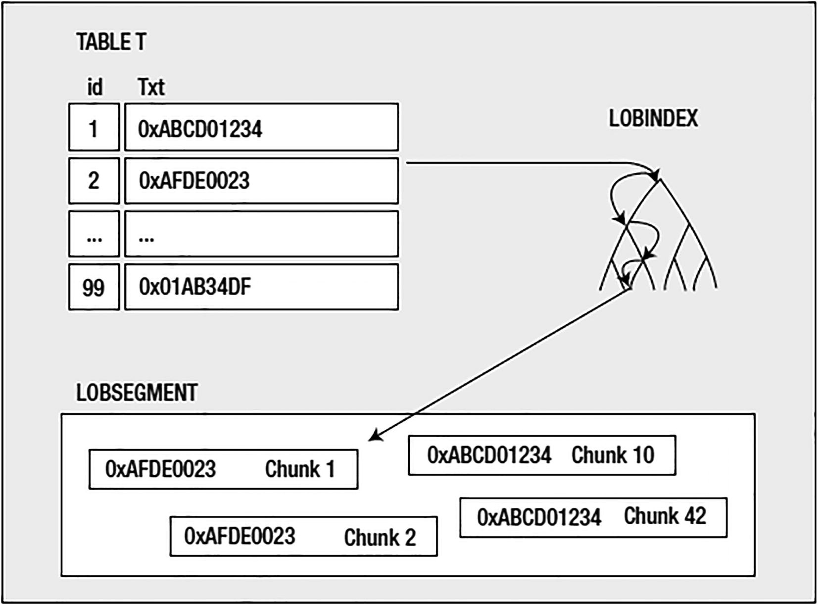
Table to LOBINDEX to LOBSEGMENT
The LOB locator in the table really just points to the LOBINDEX; the LOBINDEX, in turn, points to all of the pieces of the LOB itself. To get bytes N through M of the LOB, you would dereference the pointer in the table (the LOB locator), walk the LOBINDEX structure to find the needed chunks, and then access them in order. This makes random access to any piece of the LOB equally fast—you can get the front, the middle, or the end of a LOB equally fast, as you don’t always just start at the beginning and walk the LOB.
Now that you understand conceptually how a LOB is stored, I’d like to walk through each of the optional settings listed previously and explain what they are used for and what exactly they imply.
LOB Tablespace
The TABLESPACE specified here is the tablespace where the LOBSEGMENT and LOBINDEX will be stored, and this may be different from the tablespace where the table itself resides. That is, the tablespace that holds the LOB data may be separate and distinct from the tablespace that holds the actual table data.
The main reasons you might consider using a different tablespace for the LOB data vs. the table data are mostly administrative and performance related. From the administrative angle, a LOB datatype represents a sizable amount of information. If the table had millions of rows, and each row has a sizable LOB associated with it, the LOB data would be huge. It would make sense to segregate the table from the LOB data just to facilitate backup and recovery and space management. You may well want a different uniform extent size for your LOB data than you have for your regular table data, for example.
The other reason could be for I/O performance. By default, LOBs are not cached in the buffer cache (more on that later). Therefore, by default every LOB access, be it read or write, is a physical I/O—a direct read from disk or a direct write to disk.
LOBs may be in line or stored in the table. In that case, the LOB data would be cached, but this applies only to LOBs that are 4000 bytes or less in size. We’ll discuss this further in the section “IN ROW Clause.”
Because each access is a physical I/O, it makes sense to segregate the objects you know for a fact will be experiencing more physical I/O than most objects in real time (as the user accesses them) to their own disks.
It should be noted that the LOBINDEX and the LOBSEGMENT will always be in the same tablespace. You cannot have the LOBINDEX and LOBSEGMENT in separate tablespaces. In fact, all storage characteristics of the LOBINDEX are inherited from the LOBSEGMENT, as we’ll see shortly.
IN ROW Clause
This controls whether the LOB data is always stored separate from the table in the LOBSEGMENT or if it can sometimes be stored right in the table itself without being placed into the LOBSEGMENT. If ENABLE STORAGE IN ROW is set, as opposed to DISABLE STORAGE IN ROW, small LOBs of up to 4000 bytes will be stored in the table itself, much like a VARCHAR2 would be. Only when LOBs exceed 4000 bytes will they be moved out of line into the LOBSEGMENT.
Enabling storage in the row is the default and, in general, should be the way to go if you know the LOBs will many times fit in the table itself. For example, you might have an application with a description field of some sort in it. The description might be anywhere from 0 to 32KB of data (or maybe even more, but mostly 32KB or less). Many of the descriptions are known to be very short, consisting of a couple of hundred characters. Rather than going through the overhead of storing these out of line and accessing them via the index every time you retrieve them, you can store them in line, in the table itself. Further, if the LOB is using the default of NOCACHE (the LOBSEGMENT data is not cached in the buffer cache), then a LOB stored in the table segment (which is cached) will avoid the physical I/O required to retrieve the LOB.
Starting with Oracle 12c, you can create a VARCHAR2, NVARCHAR2, or RAW column that will store up to 32,767 bytes of information. See the “Extended Datatypes” section in this chapter for details.
The retrieval of the IN_ROW column was significantly faster and consumed far fewer resources. We can see that it used 54,720 logical I/Os (query mode gets), whereas the OUT_ROW column used significantly more logical I/Os. At first, it is not clear where these extra logical I/Os are coming from, but if you remember how LOBs are stored, it will become obvious. These are the I/Os against the LOBINDEX segment in order to find the pieces of the LOB. Those extra logical I/Os are all against this LOBINDEX.
Additionally, you can see that the retrieval of 18,240 rows with out-of-row storage incurred 18,240 physical I/Os and resulted in 18,240 I/O waits for direct path read. These were the reads of the noncached LOB data. We might be able to reduce them in this case by enabling caching on the LOB data, but then we’d have to ensure we had sufficient additional buffer cache to be used for this. Also, if there were some really large LOBs in there, we might not really want this data to be cached.
Note the increased I/O usage, both on the read and writes. All in all, this shows that if you use a CLOB, and many of the strings are expected to fit in the row (i.e., will be less than 4000 bytes), then using the default of ENABLE STORAGE IN ROW is a good idea.
CHUNK Clause
LOBs are stored in chunks; the index that points to the LOB data points to individual chunks of data. Chunks are logically contiguous sets of blocks and are the smallest unit of allocation for LOBs, whereas normally a block is the smallest unit of allocation. The CHUNK size must be an integer multiple of your Oracle block size—this is the only valid value.
The CHUNK clause only applies to BasicFiles. The CHUNK clause appears in the syntax clause for SecureFiles for backward compatibility purposes only.
You must take care to choose a CHUNK size from two perspectives. First, each LOB instance (each LOB value stored out of line) will consume at least one CHUNK. A single CHUNK is used by a single LOB value. If a table has 100 rows and each row has a LOB with 7KB of data in it, you can be sure that there will be 100 chunks allocated. If you set the CHUNK size to 32KB, you will have 100 32KB chunks allocated. If you set the CHUNK size to 8KB, you will have (probably) 100 8KB chunks allocated. The point is, a chunk is used by only one LOB entry (two LOBs will not use the same CHUNK). If you pick a chunk size that does not meet your expected LOB sizes, you could end up wasting an excessive amount of space. For example, if you have that table with 7KB LOBs on average, and you use a CHUNK size of 32KB, you will be wasting approximately 25KB of space per LOB instance. On the other hand, if you use an 8KB CHUNK, you will minimize any sort of waste.
You also need to be careful when you want to minimize the number of CHUNKs you have per LOB instance. As you have seen, there is a LOBINDEX used to point to the individual chunks, and the more chunks you have, the larger this index is. If you have a 4MB LOB and use an 8KB CHUNK, you will need at least 512 CHUNKs to store that information. This means you need at least enough LOBINDEX entries to point to these chunks. It might not sound like a lot until you remember this is per LOB instance; if you have thousands of 4MB LOBs, you now have many thousands of entries. This will also affect your retrieval performance, as it takes longer to read and manage many small chunks than it takes to read fewer, but larger, chunks. The ultimate goal is to use a CHUNK size that minimizes your waste, but also efficiently stores your data.
RETENTION Clause
The RETENTION clause differs depending on whether you’re using SecureFiles or BasicFiles. If you look back at the output of DBMS_METADATA at the beginning of the “Internal LOBs” section, notice that there is no RETENTION clause in the CREATE TABLE statement for a SecureFiles LOB, whereas there is one for a BasicFiles LOB. This is because RETENTION is automatically enabled for SecureFiles.
RETENTION is used to control the read consistency of the LOB. I’ll provide details in subsequent subsections on how RETENTION is handled differently between SecureFiles and BasicFiles.
Read Consistency for LOBs
In previous chapters, we’ve discussed read consistency, multiversioning, and the role that undo plays in that. Well, when it comes to LOBs, the way read consistency is implemented changes. The LOBSEGMENT does not use undo to record its changes; rather, it versions the information directly in the LOBSEGMENT itself. The LOBINDEX generates undo just as any other segment would, but the LOBSEGMENT does not. Instead, when you modify a LOB, Oracle allocates a new CHUNK and leaves the old CHUNK in place. If you roll back your transaction, the changes to the LOB index are rolled back, and the index will point to the old CHUNK again. So the undo maintenance is performed right in the LOBSEGMENT itself. As you modify the data, the old data is left in place and new data is created.
This comes into play for reading the LOB data as well. LOBs are read consistent, just as all other segments are. If you retrieve a LOB locator at 9:00 a.m., the LOB data you retrieve from it will be “as of 9:00 a.m.” Just like if you open a cursor (a resultset) at 9:00 a.m., the rows it produces will be as of that point in time. Even if someone else comes along and modifies the LOB data and commits (or not), your LOB locator will be “as of 9:00 a.m.,” just like your resultset would be. Here, Oracle uses the LOBSEGMENT along with the read-consistent view of the LOBINDEX to undo the changes to the LOB, to present you with the LOB data as it existed when you retrieved the LOB locator. It does not use the undo information for the LOBSEGMENT, since none was generated for the LOBSEGMENT itself.
The read-consistent images for the cursor C came from the undo segments, whereas the read-consistent images for the LOB came from the LOBSEGMENT itself. So, that gives us a reason to be concerned: if the undo segments are not used to store rollback for LOBs and LOBs support read consistency, how can we prevent the dreaded ORA-01555: snapshot too old error from occurring? And, as important, how do we control the amount of space used by these old versions? That is where RETENTION and, alternatively, PCTVERSION come into play.
BasicFiles RETENTION
RETENTION tells the database to retain modified LOB segment data in the LOB segment in accordance with your database’s UNDO_RETENTION setting. If you set your UNDO_RETENTION to two days, Oracle will attempt to not reuse LOB segment space freed by a modification. That is, if you deleted all of your rows pointing to LOBS, Oracle would attempt to retain the data in the LOB segment (the deleted data) for two days in order to satisfy your UNDO_RETENTION policy, just as it would attempt to retain the undo information for the structured data (your relational rows and columns) in the UNDO tablespace for two days. It is important you understand this: the freed space in the LOB segment will not be immediately reused by subsequent INSERTs or UPDATEs. This is a frequent cause of questions in the form of, “Why is my LOB segment growing and growing?” A mass purge followed by a reload of information will tend to cause the LOB segment to just grow, since the retention period has not yet expired.
Alternatively, the BasicFiles LOB storage clause could use PCTVERSION, which controls the percentage of allocated (used by LOBs at some point and blocks under the LOBSEGMENT’s HWM) LOB space that should be used for versioning of LOB data. The default of ten percent is adequate for many uses since many times you only ever INSERT and retrieve LOBs (updating of LOBs is typically not done; LOBs tend to be inserted once and retrieved many times). Therefore, not much space, if any, needs to be set aside for LOB versioning.
and increase the amount of space to be used in that LOBSEGMENT for versioning of data.
SecureFiles RETENTION
SecureFiles use RETENTION to control read consistency (just like BasicFiles). In the CREATE TABLE output of DBMS_METADATA for the SecureFiles LOB, there is no RETENTION clause. This is because the default RETENTION is set to AUTO, which instructs Oracle to retain undo long enough for read-consistent purposes.
Use MAX to indicate that the undo should be retained until the LOB segment has reached the MAXSIZE specified in the storage clause (therefore, MAX must be used in conjunction with the MAXSIZE clause in the storage clause).
Set MIN N if the Flashback Database is enabled to limit the undo duration for the LOB to N seconds.
Set NONE if undo is not required for consistent reads or flashback operations.
If you don’t set the RETENTION parameter for SecureFiles, or specify RETENTION with no parameters, then it is set to DEFAULT (which is the equivalent of AUTO).
CACHE Clause
The alternative to NOCACHE is CACHE or CACHE READS. This clause controls whether or not the LOBSEGMENT data is stored in the buffer cache. The default NOCACHE implies that every access will be a direct read from disk, and every write/modification will likewise be a direct read from disk. CACHE READS allows LOB data that is read from disk to be buffered, but writes of LOB data will be done directly to disk. CACHE permits the caching of LOB data during both reads and writes.
to see the effect this may have on you. For a large initial load, it would make sense to enable caching of the LOBs and allow DBWR to write the LOB data out to disk in the background while your client application keeps loading more. For small- to medium-sized LOBs that are frequently accessed or modified, caching makes sense so the end user doesn’t have to wait for physical I/O to complete in real time. For a LOB that is 50MB in size, however, it probably does not make sense to have that in the cache.
Bear in mind that you can make excellent use of the keep or recycle pools (discussed in Chapter 4) here. Instead of caching the LOBSEGMENT data in the default cache with all of the regular data, you can use the keep or recycle pools to separate it out. In that fashion, you can achieve the goal of caching LOB data without affecting the caching of existing data in your system.
LOB STORAGE Clause
Both SecureFiles and BasicFiles have a full storage clause you can employ to control the physical storage characteristics. It should be noted that this storage clause applies to the LOBSEGMENT and the LOBINDEX equally—a setting for one is used for the other.
The management of the storage with SecureFiles is less complicated than that of a BasicFiles. Recall that a SecureFiles LOB must be created within an ASSM-managed tablespace, and therefore the following attributes no longer apply: FREELISTS, FREELIST GROUPS, and FREEPOOLS.
For a BasicFiles LOB, the relevant settings for a LOB would be the FREELISTS and FREELIST GROUPS (when not using ASSM, as discussed in Chapter 10). The same rules apply to the LOBINDEX segment, as the LOBINDEX is managed the same as any other index segment. If you have highly concurrent modifications of LOBs, multiple FREELISTS on the index segment might be recommended.
As mentioned in the previous section, using the keep or recycle pools for LOB segments can be a useful technique to allow you to cache LOB data, without damaging your existing default buffer cache. Rather than having the LOBs age out block buffers from normal tables, you can set aside a dedicated piece of memory in the SGA just for these objects. The BUFFER_POOL clause could be used to achieve that.
BFILEs
The last of the LOB types to talk about is the BFILE type . A BFILE type is simply a pointer to a file in the operating system. It is used to provide read-only access to these operating system files.
The built-in package UTL_FILE provides read and write access to operating system files, too. It does not use the BFILE type, however.
I recommend against using quoted identifiers; rather, use the uppercase name in the BFILENAME call. Quoted identifiers are not usual and tend to create confusion downstream.
A BFILE (the pointer object in the database, not the actual binary file on disk) consumes a varying amount of space on disk, depending on the length of the DIRECTORY object name and the file name. In the preceding example, the resulting BFILE was about 35 bytes in length. In general, you’ll find the BFILE consumes approximately 20 bytes of overhead plus the length of the DIRECTORY object name plus the length of the file name itself.
BFILE data is not read consistent as other LOB data is. Since the BFILE is managed outside of the database, whatever happens to be in the file when you dereference the BFILE is what you will get. So, repeated reads from the same BFILE may produce different results—unlike a LOB locator used against a CLOB, BLOB, or NCLOB.
ROWID/UROWID Types
The last datatypes to discuss are the ROWID and UROWID types . A ROWID is the address of a row in a table (remember from Chapter 10 that it takes a ROWID plus a table name to uniquely identify a row in a database). Sufficient information is encoded in the ROWID to locate the row on disk, as well as identify the object the ROWID points to (the table and so on). ROWID’s close relative, UROWID, is a universal ROWID and is used for tables, such as IOTs and tables accessed via gateways to heterogeneous databases that do not have fixed ROWIDs. The UROWID is a representation of the primary key value of the row and hence will vary in size depending on the object it points to.
Every row in every table has either a ROWID or a UROWID associated with it. They are considered pseudo columns when retrieved from a table, meaning they are not actually stored with the row, but rather are a derived attribute of the row. A ROWID is generated based on the physical location of the row; it is not stored with it. A UROWID is generated based on the row’s primary key, so in a sense it is stored with the row, but not really, as the UROWID does not exist as a discrete column, but rather as a function of the existing columns.
Updating the partition key of a row in a partitioned table such that the row must move from one partition to another
Using the FLASHBACK table command to restore a database table to a prior point in time
MOVE operations and many partition operations such as splitting or merge partitions
Using the ALTER TABLE SHRINK SPACE command to perform a segment shrink
Now, since ROWIDs can change over time (since they are no longer immutable), it is not recommended to physically store them as columns in database tables. That is, using a ROWID as a datatype of a database column is considered a bad practice and should be avoided. The primary key of the row (which should be immutable) should be used instead, and referential integrity can be in place to ensure data integrity is preserved. You cannot do this with the ROWID types—you cannot create a foreign key from a child table to a parent table by ROWID, and you cannot enforce integrity across tables like that. You must use the primary key constraint.
Of what use is the ROWID type, then? It is still useful in applications that allow the end user to interact with the data—the ROWID, being a physical address of a row, is the fastest way to access a single row in any table. An application that reads data out of the database and presents it to the end user can use the ROWID upon attempting to update that row. The application must use the ROWID in combination with other fields or checksums (refer to Chapter 7 for further information on application locking). In this fashion, you can update the row in question with the least amount of work (e.g., no index lookup to find the row again) and ensure the row is the same row you read out in the first place by verifying the column values have not changed. So, a ROWID is useful in applications that employ optimistic locking.
JSON Type
New in 21c, Oracle introduces the JSON datatype . This datatype allows you to store JSON data natively in binary format in the database. It is an optimized binary storage that uses the OSON format. The OSON format is Oracle’s optimized binary JSON format. Using this format, query performance is greatly enhanced because textual JSON data is no longer parsed. The JSON datatype can be declared for a table, a materialized view, and PL/SQL parameters.
In this manner, you can store and retrieve JSON data in its native binary format in the database. This allows for improved query performance when dealing with JSON data. This is because the data is not stored as text and therefore doesn’t need to be parsed.
Summary
In this chapter, we’ve examined many basic datatypes provided by Oracle; we’ve seen how they are physically stored and what options are available with each. We started with character strings, the most basic of types, and looked into considerations surrounding multibyte characters and raw binary data. We then discussed extended datatypes (available in Oracle 12c and above) and how this feature allows you to define VARCHAR2, NVARCHAR2, and RAW datatypes to be as large as 32,727 bytes. Next, we studied the numeric types, including the very precise Oracle NUMBER type and the floating-point types provided with Oracle.
We also gave consideration to the legacy LONG and LONG RAW types, concentrating on how you might work around their existence, as the functionality provided by these types falls far short of that provided by the LOB types. Next, we looked at the datatypes capable of storing dates and times. We covered the basics of date arithmetic, a perplexing issue until you’ve seen it demonstrated. Lastly, in the section on dates and timestamps, we looked at the INTERVAL type and how best to use it.
The most detailed part of the chapter from a physical storage perspective was the LOB section. The LOB type is frequently misunderstood by developers and DBAs alike, so the bulk of the section was spent looking at how they are physically implemented as well as certain performance considerations and the differences between SecureFiles and BasicFiles.
We also looked at the ROWID/UROWID type. For what now should be obvious reasons, you should not use this datatype as a database column, since ROWIDs are not immutable and no integrity constraints could enforce the parent/child relationship. Rather, you want to store primary keys if you need to point to another row.
The last datatype we examined was the JSON datatype. This new datatype was introduced in Oracle 21c. This allows you to store JSON data in a native binary format within the database. This improves query performance as you don’t have to parse the data when retrieving it (like you would if it was stored as text).